

Abstract
Metabolomics is the science of characterizing and quantifying small molecule metabolites in biological systems. These metabolites give organisms their biochemical characteristics, providing a link between genotype, environment and phenotype. With these opportunities also come data challenges, such as compound annotation, missing values and batch effects. We present the steps of a general pipeline to process untargeted mass spectrometry data to alleviate the latter two challenges. We assume to have a matrix with metabolite abundances, with metabolites in rows and samples in columns. The steps in the pipeline include summarizing technical replicates (if available), filtering, imputing, transforming and normalizing the data. In each of these steps, a method and parameters should be chosen based on assumptions one is willing to make, the question of interest, and diagnostic tools. Besides giving a general pipeline that can be adapted by the reader, our goal is to review diagnostic tools and criteria that are helpful when making decisions in each step of the pipeline and assessing the effectiveness of normalization and batch correction. We conclude by giving a list of useful packages and discuss some alternative approaches that might be more appropriate for the reader’s data.
Keywords: Mass spectrometry, untargeted, metabolomics, processing, pre-analytic, technical replicates, filtering, imputation, normalization
1. Introduction
Metabolomics is concerned with the comprehensive characterization and quantification of small molecule metabolites in biological systems; the metabolites present in a sample or system are referred to as the metabolome (see (1, 2) and http://www.metabolomicssociety.org/). Metabolomics allows for an assessment of a cellular state within the context of the environment (see (2–5) and references therein) and gives complementary insight into biological processes as compared to genomics and proteomics (see (2, 3, 6)). Metabolites can also serve as markers of disease severity and drug sensitivity (2, 7–10). Thus, metabolites give organisms their biochemical characteristics, providing a link between genotype, environment, and phenotype.
Metabolomics can be classified as targeted or untargeted. Targeted metabolomics measures only smaller, defined groups of chemically characterized and biochemically annotated metabolites, while untargeted metabolomics is designed to comprehensively measure analytes in a sample, including chemical unknowns. In addition, internal standards can be included in both approaches for absolute quantification and/or to evaluate technical variation. In the following, we focus on untargeted metabolomics and will refer to it simply as metabolomics. We will also use the terms metabolites and compounds interchangeably.
We focus on liquid chromatography mass spectrometry (LC-MS), but much of the discussion applies to other MS applications, such as gas chromatography and LC-MS based proteomics data. The main alternative to MS is nuclear magnetic resonance (NMR) spectroscopy (12, 13). Both MS and NMR technologies have their strengths and weaknesses, supplementing and complementing each other (12–14): For example, MS is more sensitive than NMR and can detect lower-abundance metabolites. NMR, on the other hand is better at determining the structure of unknown metabolites, is non-destructive, and can be used in vivo.
While MS based metabolomics brings many opportunities, the complexity of the metabolome and technical limitations also bring challenges. The challenges we focus on here are missing values and unwanted variation, such as batch effects; annotation of compounds is another challenge that we only discuss in the context of missing values. These challenges occur also in other omics fields such as transcriptomics, and tools that have been developed there are often adapted or directly used for metabolomics data. For example ComBat was developed to “combat” batch effects in gene expression microarray data (15–17), but it has been used in a variety of fields, including metabolomics (see (18) and references therein). On the other hand, there are also many MS specific tools for metabolomic data. An example for a normalization method using internal standards is Cross-contribution Compensating Multiple standard Normalization (CCMN )(19). Another MS specific normalization method, using quality control samples, is the mixture model normalization implemented in Metabomxtr (20, 21).
Our goal is to make the reader aware of some of the challenges in MS based metabolomics data and ways to evaluate and/or alleviate their impact on downstream analyses and results. In particular, we aim to provide the reader with a pipeline for “cleaning” the data for statistical analysis.
The challenges in MS based metabolomics data we discuss here are missing values, right-skewness of data, batch and run-order effects and other unwanted variation. Batches often refer to the set of samples run on a particular date, and signal intensities can vary between these batches. Within a batch, run-order effects refer to changes in signal intensities over the different MS runs within a batch. We will return to this when discussing normalization methods.
To address these challenges, we use the pre-analytic pipeline outlined in Figure 1. We think of pre-analytic processing as the steps starting with a data matrix containing metabolites or compounds in rows and samples, including technical replicates if available, in columns. Note that compounds are characterized by two measurements, retention time and mass. Retention time is the time from injection of the sample to the top of the peak for each compound of interest (22). The mass of a compound can be used to determine the kind and number of atoms in the molecule. The same compound can have different retention times in different samples, resulting in uncertainty of whether signals from two or more samples correspond to the same metabolite. For a discussion of this peak-shift problem, causes and alignment methods see e.g. (23, 24).
Figure 1. Pre-analytic pipeline.
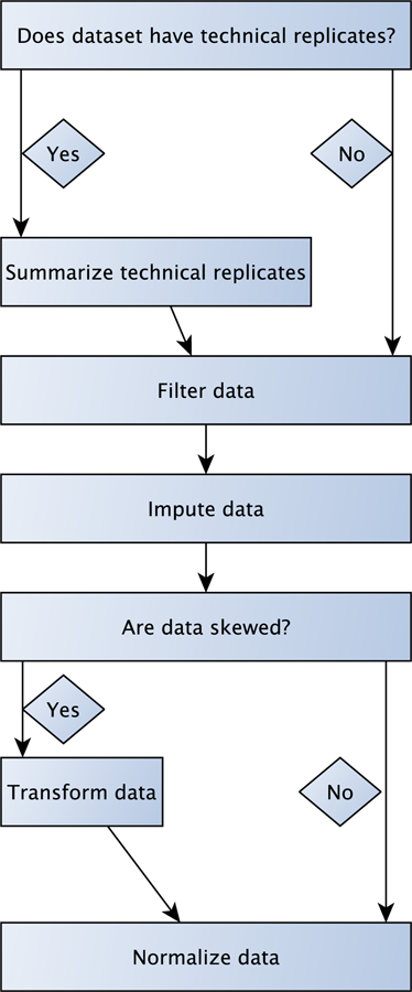
The five individual pipeline steps are discussed in more detail in Sections 2.1–2.5, with each section corresponding to one step.
Pre-analytic processing pipeline:
The steps we consider to be important parts of a pre-analytic processing pipeline are as follows:
Summarization of technical replicates (if available)
Filtering of metabolites
Imputation of missing values
Transformation of data
Normalization and batch correction
Note that these steps are often referred to as pre-processing. To avoid confusion with the pre-processing upstream (peak finding, annotation, etc.), we use the term pre-analytic. The individual challenges and approaches to alleviate them are discussed in the Methods section below.
Example dataset:
For illustration purposes, we use data generated from subjects from the COPDGene genetic epidemiology study (25). Chronic obstructive pulmonary disease (COPD) is characterized by several clinical phenotypes, including airflow obstruction, emphysema, chronic bronchitis, and frequent exacerbations (see (9, 10) and references therein). Smoking is the major risk factor, but most smokers do not develop COPD (10). Links between alterations in sphingolipid metabolism and disease susceptibility were suggested (9, 26, 27). For 131 plasma samples from current and former smokers in COPDGene, the lipid fraction was analyzed, using an ultra-high performance liquid chromatograph (Agilent 1290 Series) and a time-of-flight mass spectrometer (Agilent 6210), which resulted in data on 6166 features. For more detailed information about the cohort and data generation, see (10).
2. Methods
In this section, we go through the five pipeline steps (Figure 1) in detail. We use the MSPrep package (28), which implements or uses existing packages of the discussed methods; however, note that all steps can be performed without using MSPrep. Within certain steps, we illustrate a specific method using diagnostic plots and our motivating data set but note that different options may be appropriate for other data sets. We also give short explanations for major sources of challenges as well as our rationale for the chosen pipeline steps. We will focus more on the importance of these pre-analytic steps rather than on the specific method used at individual steps. For reviews, evaluations, and discussions of the methods see e.g. (20, 29–34) and references therein. Finally, in the Notes section, we will discuss alternatives and challenges.
2.1. Summarization of technical replicates
Many studies use technical replicates, which are repeated runs of the same sample through the mass spectrometer. The benefits of technical replicates include the ability to obtain a more precise and robust measurement of a biological sample if we run it through the mass spectrometer multiple times and use the median or mean intensity as the final measurement. In particular, this could help with missing values if a metabolite was measured in a certain number of technical replicates; details and references are provided in our example summarization and Notes 3–4. The variability of the technical replicates can also be used to determine if the metabolite could be measured with high or low accuracy, as measured by the coefficient of variation.
However, technical replicates are not always performed due to cost or lack of available material. The downside of technical replicates is the increased complexity in the peak alignment process, as discussed above, which could result in more “duplicated” metabolites (i.e. rows in our data with metabolites having same mass and estimated chemical formula, but retention times that are sufficiently different for the software to consider the metabolites as being separated). Other disadvantages include fewer biological samples that can fit in a batch, and the need for additional analyses steps.
Example of summarization of technical replicates:
In our data, three technical replicates were randomized within each batch. We examined the missingness and variability of metabolite measurements using the coefficient of variation (CV) in the technical replicates. For a sample, the CV is defined as the standard deviation divided by the mean. When using the CV as criterion for acceptable variation in the measurements, we account for the fact that the standard deviation naturally increases with the mean. Based on missingness and CV, technical replicates were summarized (see Figure 2). For the COPD data, we counted how often there were 0, 1, 2, or 3 missing values in the respective technical replicates across all samples and metabolites (Table 1). Across all metabolites and samples combinations, approximately 60% had less than two missing values. If two out of three replicates have a missing value, then we assign a missing value to the metabolite in that sample; for a discussion, see e.g. (35, 36). When there were at least two non-missing values, we then examine the CV as summarization criterion because our rationale is that low variability indicates that the metabolite could be measured accurately and that in this case the missing value (if any) might well be due to technical issues. In this setting, summarizing the replicates as mean or median depending on the CV will reduce the run-order effect. In Notes 3–4, we discuss alternatives to this approach.
Figure 2. Example of summarization of technical replicates.

For each metabolite and sample, we calculate the coefficient of variation (CV). If two or more replicates have a missing value, we assign a missing value to the metabolite for this sample. If at most one of the three values is missing, and the CV is low (≤0.5), we summarize the replicates with the mean. If the CV is high (>0.5) and we have a missing value, we conclude that the metabolite cannot be measured accurately and we assign a missing value. With a high CV and no missing values, we choose the median as a robust summary of the replicates.
Table 1.
Missingness in technical replicates across all samples and metabolites. The number of missing values across the three technical replicates is summarized by the count of metabolite-sample combinations and by the overall percent.
| # missing values | count | percent |
|---|---|---|
| 0 | 373965 | 46.19 |
| 1 | 98457 | 12.16 |
| 2 | 95945 | 11.85 |
| 3 | 241213 | 29.79 |
2.2. Filtering
In this work, we refer to filtering as the removal of metabolites if there are too many missing values across samples. Using our example dataset, after summarization of the technical replicates, we examined the distribution of missingness in our COPD data and found that although there was a large number of metabolites with very few missing values, 2682 (43.5%) of the metabolites had more than 50% missing (Figure 3).
Figure 3.
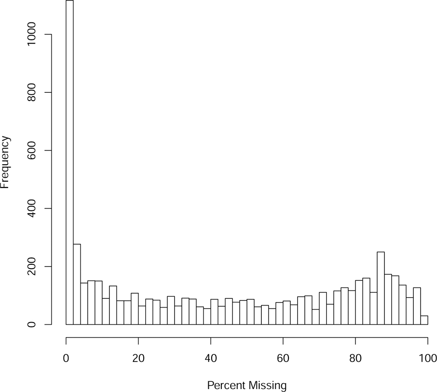
After summarization of replicates, histogram of missingness across samples for each of the 6166 metabolite features.
To understand the need for filtering and the impact of imputation for downstream steps in the pipeline, we briefly discuss the reasons for missing values. Missingness is often classified as missing completely at random (MCAR), missing at random (MAR), and missing not at random (MNAR) (see (37, 38)): MCAR means that each measurement is equally likely to have a missing value, that is, there is no systematic difference between missing and non-missing data. MAR means that the probability that a value is missing only depends on observed data of other variables measured, that is any systematic difference between missing and non-missing data can be explained by differences in observed data. MNAR means that after the observed data (of all measured variables) are taken into account, systematic differences remain between the missing and non-missing values.
Missingness in untargeted MS data can have the following reasons:
Metabolite is not present.
Metabolite is below detection threshold.
Other technical reasons, such as misalignment of the detected peaks.
These reasons can partially be classified using the “missingness mechanisms” described above: MCAR, MAR, and MNAR. For metabolites that are not present or below the detection threshold, the data are MNAR. If the data is missing for other technical reasons, the probability of missingness can, for example, depend on m/z (33), which is a measureable quantity. If the probability of missingness were completely determined by m/z, then this would be attributed to MAR. However, missingness is also intensity (abundance) dependent (33), which means there is an MNAR component. This is in contrast to MCAR, where the probability of missingness does not depend on measureable or un-measureable quantities. It is often difficult or impossible to determine what mechanism caused the missing value. However, understanding the sources of missingness helps to understand the potential biases introduced by imputation, which is discussed below.
Filtering.
If a metabolite has too many missing values, it might not be present in many samples, is very low abundant, or generally hard to quantify. In that case, it might be best to remove that metabolite. There is no consensus on the right filter, but in our experience filtering out the metabolites that have less than 80% non-missing values strikes a good balance of obtaining a relatively “clean” data set for which imputation and normalization will work reasonably well; this was termed “80%” rule in (39) where 80% of the metabolites were required to be present within each group. When there are too many missing values, imputation might not work very well. Restricting ourselves to allow fewer missing values could result in losing too many potentially important metabolites (see (36) and references therein). In our COPD data we have 6166 metabolite features before filtering. Allowing for weak filtering, (up to 40% missing values), this reduces the number of metabolites to 3084 (~50% of the original metabolites). More stringent filtering (up to 20% missing values) results in 2333 metabolites (~38% of original metabolites). See Notes 2, 5–7 for alternative approaches.
2.3. Imputation
Many downstream analyses, such as classification, require complete data. Imputation refers to the estimation of missing values.. There is a wide selection of imputation strategies available, each of which has their own assumptions about the nature of missing values. The impact on downstream analyses, such as differential abundance, has been noted in the literature (see e.g. (33)). For example, a simple imputation method is to replace missing values with a small value, such as zero, the minimum observed value in other samples, or half the minimum. These imputation methods might be appropriate if missingness is due to low abundance or absence of the metabolite. If missingness is due to other technical issues and the metabolite is present at high abundance but not detected, these imputation methods cause bias and can cause high variability if the metabolite is abundantly present and detected in the other samples.
As an example application, we use k-nearest neighbors (kNN) imputation. Roughly, for the sample that is missing a particular metabolite M, the k samples that have the most similar metabolite values (profile) will be considered, and the median of their abundances for metabolite M is used to impute the missing value (40). Other popular imputation methods are Bayesian PCA (BPCA) (41) and random forest (42). Recent articles reviewing and evaluating these and other methods are (32, 34). See also Notes 8–9 for additional discussion.
2.4. Transforming the data
Metabolomics data is typically right-skewed and heteroscedastic. The latter refers to unequal variance of observations across samples; in right-skewed data, variance often increases with the (average) value of the measurement. These characteristics of the data may violate assumptions for standard statistical analyses. A simple and widely used transformation to make data more symmetric and homoscedastic is the log-transformation (see e.g. (43)). We recommend this as the default choice and discuss alternatives and evaluation tools in Notes 10–11 (see also (43)). An illustrative example of the effect of a log2-transformation for an example metabolite is presented in Figure 4. We used the log2-transformation on our COPDGene data.
Figure 4.
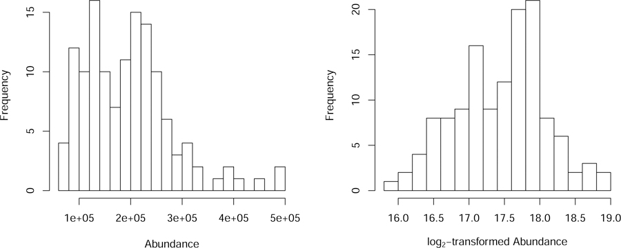
Distribution of example metabolite (sphingosine) abundance before (left panel) and after log2-transformation (right panel).
2.5. Normalization and batch correction
Batch and run-order effects.
Similar to other omics technologies, MS suffers from batch effects. As mentioned above, batches often refer to the set of samples run on a particular date. In principle, one could run the machine longer and increase the “batch” size. Besides batch effects, run-order effects within a batch can be observed, and both batch and run-order effects can be metabolite specific (see e.g. (20)).
Normalization.
To alleviate batch effects and other unwanted variation, the data should be normalized so that different samples can be compared. Similar to imputation strategies, a variety of normalization methods are available, again each with their own assumptions. For recent discussions of methods, see e.g. (20, 29–32) and references therein. A simple yet effective first step is typically a median normalization, which aligns the median signal of all metabolites across samples. The assumption is that most of the metabolites do not change considerably across samples (see also Notes 12–16). While median normalization typically removes some unwanted variation, other unwanted variation usually remains, some of which are often due to batch effects. The latter can be reduced using, for example, ComBat (15). Some other popular methods to reduce unwanted variation are Surrogate Variable Analysis (SVA) (16, 44), Remove Unwanted Variation (RUV) (45), and Cross-contribution Compensating Multiple standard Normalization (CCMN) (19). Normalization methods can also be based on quality control (QC) samples, as for example in (20, 21). See Notes 12–16 for additional discussions. Diagnostic tools, discussed next, can guide the choice of normalization methods.
Diagnostic tools
Diagnostic tools allow us to evaluate the effect of different normalization methods and can help guide our choice of normalization methods. We will discuss relative log expression (RLE) plots and PCA plots. Limitations of these tools, as well as heatmaps combined with hierarchical clustering will be discussed in Note 16.
RLE plots:
Relative log expression plots were originally developed to analyze microarray gene expression data (46–48). These are boxplots of transformed and centered abundance data. More precisely, after log-transforming the abundances, for a given sample and metabolite we subtract the median of the log-abundances across all samples. These plots are often better at revealing heterogeneity between samples and batches than boxplots based on log(yij) without subtracting the median. A discussion using real and simulated data can be found in (46). We adapt their discussion to our situation. Assume the following:
The abundances of a majority of metabolites are unaffected by the biological factors of interest.
For each metabolite i that satisfies Assumption (1), the distribution of log(yij) is approximately symmetric.
For a metabolite i satisfying these assumptions, the distribution of the transformed abundances is approximately centered at zero and has constant variance for j = 1, … , n, where n is the sample size. In particular, the RLE plots should be approximately centered at 0 and have comparable interquartile ranges if the above assumptions are satisfied.
PCA plots:
Principal component analysis determines, roughly speaking, the orthogonal directions of maximal variation in the data. Often, the data will then be projected onto the 2- or 3-dimensional space spanned by these directions of maximal variation or principal components (PCs). For an overview article of PCA, see (49). If the samples cluster by batches in these plots, that means a high amount of variation in the data stems from batch effects. These clustered batches can often be seen in the data before normalization. After normalization, these clusters should be closer together and their difference minimized.
Illustrative example:
In our COPDGene data, we observe batch effects before normalization. After a median and ComBat normalization, these effects are alleviated (Figures 5 and 6). In particular, we observe in the RLE plots that before normalization, the boxplots of some batches tend to be centered above or below zero, while after normalization, all boxplots are roughly centered at zero (Figure 5). Similarly, in the PCA plots, we observe strong batch effects before normalization. The batch effect is alleviated after normalization (Figure 6).
Figure 5. RLE Plots.
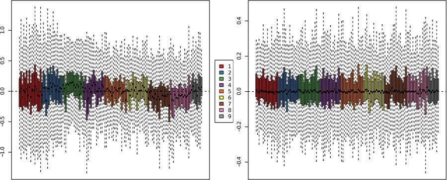
The kNN-imputed data before normalization (left panel). The kNN-imputed data after median and ComBat normalization (right panel). The nine batches are color-coded. The kNN imputation was done using the VIM R package, with k=5 (40). The RLE plot was produced using plotRLE in the EDASeq package (57).
Figure 6. PCA Plots.
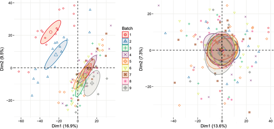
The kNN-imputed data before normalization (left panel) and after median and ComBat normalization (right panel). The PCA plot was produced using the factoextra package (58).
2.6. Concluding remarks
The pre-analytic pipeline is used to prepare the data for downstream analyses, such as differential abundance analysis of metabolites between two groups, regression analysis to determine associations between phenotypes and metabolites, classification using metabolite profiles, and pathway analysis, to name a few. While the downstream analysis is beyond the scope of this chapter, we want to emphasize that the chosen pre-analytic steps and methods will have an impact on downstream analyses. Sensitivity analyses can be performed to evaluate the impact of various pre-analytic steps on downstream results. For reviews, evaluations, and discussions of pre-analytic steps, as well as their impact on downstream results, see e.g. (20, 29–34) and references therein.
We conclude with a table of selected free and/or open source tools that implement normalization methods (Table 2).
Table 2. Selected free and/or open-source tools and packages for imputation and normalization.
CRAN packages are available at https://cran.r-project.org and BioConductor packages are available at https://www.bioconductor.org.
| Method/Software | Link and/or package | Reference |
|---|---|---|
| Imputation methods: | ||
| kNN | CRAN (VIM) | (40) |
| Bayesian PCA | Bioconductor (pcaMethods) | (41, 59, 60) |
| Probabilistic PCA | Bioconductor (pcaMethods) | (59) |
| Random forest imputation | CRAN (randomForest) | (42) |
| MetaboAnalyst | http://www.metaboanalyst.ca/ | (53) |
| Normalization methods: | ||
| ComBat | Bioconductor (sva) | (15–17, 44) |
| Cross-contribution Robust Multiple standard Normalization | CRAN (crmn) | (19) |
| EigenMS | https://sourceforge.net/projects/eigenms/ (EigenMS R package) | (61, 62) |
| Metabomxtr | Bioconductor (Metabomxtr) | (20, 21) |
| MetaboQC | CRAN (MetaboQC) | (63) |
| MetNorm | CRAN (MetNorm) | (64, 65) |
| MSPrep | https://sourceforge.net/projects/msprep/ (MSPrep R package) | (28) |
| Remove Unwanted Variation | CRAN (ruv) | (45) |
| Support Vector Regression Normalization | http://www.metabolomics-shanghai.org/ (MetNormalizer R package) | (66) |
| Surrogate Variable Analysis | CRAN (sva) | (16, 44) |
| MetaboAnalyst | http://www.metaboanalyst.ca/ | (53) |
4. Acknowledgements
DR, SJ, and KK were supported by NIH/NHLBI Grant Number P20 HL113445. DR, DG, and KK were supported by NIH/NCATS Colorado CTSA Grant Number UL1 TR002535. HP-L was supported by training grant T15 LM009451. Contents are the authors’ sole responsibility and do not necessarily represent official NIH views.
3 Notes
Following some general notes, we provide specific comments corresponding to the individual steps in our pipeline.
3.0 General Notes
MS technologies and data processing methods constantly evolve, and we encourage the user to read the most current methods and review articles.
It is not clear if imputation or normalization should be performed first. Imputation and normalization affect each other, and while imputation works better if there is less unwanted variation such as batch effects, some normalization methods need complete data. We present imputation followed by normalization for the methods applied to our example data set. However, before proceeding with an analysis, we recommend that a user check whether a normalization method can handle missing values, and also be aware of the assumptions regarding the form of the data for an imputation method.
3.1 Notes on Summarization of Technical Replicates
For the pipeline in Figure 2, we required the metabolite to be present in at least two of the three technical replicates. An alternative is to require it to be present in all three replicates (see (36, 50, 51)).
When summarizing the technical replicates that are randomized within batches or across batches, we also lose the ability to model the run-order or batch effect using these replicates. In case the technical replicates were run back-to-back, the run-order is preserved.
3.2 Notes on Filtering
We discussed and used a “global” filtering approach, in which we removed any metabolite that has at least 80% non-missing values. See (36) for a review of other proposed filters, of requiring 50% (52) and 60%−75% (35) presence.
If there are specified subject groups of interest, an alternative approach is to filter within groups (39) or consider a present/ absent analysis. For example, given two groups (e.g. cases and controls or treatment and placebo), it could be of interest whether metabolites are present in one group but not in the other group. In a present/absent analysis the data are dichotomized, for example using a logistic regression framework. This would only work for larger sample sizes.
In metabolomics and other -omics data sets, investigators may also filter by low variance, low overall abundance, or other characteristics; see e.g. (53) and references therein.
3.3 Notes on Imputation
As discussed, imputing missing values with a small value can cause bias if the metabolite is highly abundant but not detected. Other methods, such as kNN, can cause bias as well, for example if the metabolite is indeed not present but a larger value is imputed.
Nearest neighbors imputation can be based on different distances to determine nearest neighbors and the imputed value could take different forms, such as median or mean. A modified version of kNN that accounts for truncation at the minimum value was introduced in (54).
3.4 Notes on Transformations
While a log transformation typically results in more symmetrically distributed data, there are alternative methods to transform the data to make the data more symmetric and homoscedastic. A powerful tool is the Box-Cox transformation (55). From a one or two parameter family of power transformations, with the log transformation as limit, a parameter is estimated. The data is transformed accordingly.
If the sample size is small, determining the most appropriate transformation might not be possible using statistical tests, and even visual assessment of the distributions of metabolites before and after a transformation might not result in a clear decision on the transformation. In this case, we recommend using the log transformation as discussed above.
3.5 Notes on Normalization
An alternative to median normalization is 3rd quartile normalization, which might be more robust if there are many missing values.
The assumption for median normalization and other methods is that most metabolites do not change considerably across samples. Although this may be appropriate for our example study, this assumption may not hold for other studies that have substantial global changes across the metabolome (e.g., perturbation studies).
Quality control samples, which are pooled samples and thus should only show technical variability across MS runs, can be used for normalization. In particular, if QC samples are run in different batches and at different run-order positions, they can be used to estimate run-order and batch effects (20, 21).
Assumptions for normalization methods are often not verifiable, and one has to choose the one that seems plausible and “works well” for the data. While diagnostic tools can help us determine if we were successful in removing unwanted variation, they cannot tell us if we also removed biological variation of interest or introduced other artifacts. See e.g. (46) for a more detailed discussion.
Heatmaps and hierarchical clustering of the samples can also be used to look for similarities and differences in metabolite profiles. This can be used as a diagnostic tool to assess normalization methods. If samples cluster by batches (similar to the clusters in PCA), then further normalization might be needed. For a review of heatmaps, see e.g. (56).
5. References
- 1.Jordan KW, Nordenstam J, Lauwers GY, Rothenberger DA, Alavi K, Garwood M, Cheng LL. Metabolomic Characterization of Human Rectal Adenocarcinoma with Intact Tissue Magnetic Resonance Spectroscopy. Diseases of the Colon & Rectum. 2009;52(3):520–5. doi: 10.1007/DCR.0b013e31819c9a2c. [DOI] [PMC free article] [PubMed] [Google Scholar]
- 2.Spratlin JL, Serkova NJ, Eckhardt SG. Clinical Applications of Metabolomics in Oncology: A Review. Clinical Cancer Research. 2009;15(2):431. [DOI] [PMC free article] [PubMed] [Google Scholar]
- 3.Griffin JL, Shockcor JP. Metabolic profiles of cancer cells. Nature Reviews Cancer. 2004;4:551. doi: 10.1038/nrc1390. [DOI] [PubMed] [Google Scholar]
- 4.Mendes P, Kell DB, Westerhoff HV. Why and when channelling can decrease pool size at constant net flux in a simple dynamic channel. Biochimica et Biophysica Acta (BBA) - General Subjects. 1996;1289(2):175–86. doi: 10.1016/0304-4165(95)00152-2. [DOI] [PubMed] [Google Scholar]
- 5.Mendes P, Kell DB, Westerhoff HV. Channelling can decrease pool size. European Journal of Biochemistry. 2005;204(1):257–66. doi: 10.1111/j.1432-1033.1992.tb16632.x. [DOI] [PubMed] [Google Scholar]
- 6.Boros LG, Lerner MR, Morgan DL, Taylor SL, Smith BJ, Postier RG, Brackett DJ. [1,2–13C2]-D-Glucose Profiles of the Serum, Liver, Pancreas, and DMBA-Induced Pancreatic Tumors of Rats. Pancreas. 2005;31(4). [DOI] [PubMed] [Google Scholar]
- 7.El-Deredy W, Ashmore SM, Branston NM, Darling JL, Williams SR, Thomas DGT. Pretreatment Prediction of the Chemotherapeutic Response of Human Glioma Cell Cultures Using Nuclear Magnetic Resonance Spectroscopy and Artificial Neural Networks. Cancer Research. 1997;57(19):4196. [PubMed] [Google Scholar]
- 8.Griffin JL, Pole JCM, Nicholson JK, Carmichael PL. Cellular environment of metabolites and a metabonomic study of tamoxifen in endometrial cells using gradient high resolution magic angle spinning 1H NMR spectroscopy. Biochimica et Biophysica Acta (BBA) - General Subjects. 2003;1619(2):151–8. doi: 10.1016/S0304-4165(02)00475-0. [DOI] [PubMed] [Google Scholar]
- 9.Bahr TM, Hughes GJ, Armstrong M, Reisdorph R, Coldren CD, Edwards MG, Schnell C, Kedl R, LaFlamme DJ, Reisdorph N, Kechris KJ, Bowler RP. Peripheral blood mononuclear cell gene expression in chronic obstructive pulmonary disease. Am J Respir Cell Mol Biol. 2013;49(2):316–23. doi: 10.1165/rcmb.2012-0230OC. [DOI] [PMC free article] [PubMed] [Google Scholar]
- 10.Bowler RP, Jacobson S, Cruickshank C, Hughes GJ, Siska C, Ory DS, Petrache I, Schaffer JE, Reisdorph N, Kechris K. Plasma sphingolipids associated with chronic obstructive pulmonary disease phenotypes. Am J Respir Crit Care Med. 2015;191(3):275–84. doi: 10.1164/rccm.201410-1771OC. [DOI] [PMC free article] [PubMed] [Google Scholar]
- 11.Roberts LD, Souza AL, Gerszten RE, Clish CB. Targeted Metabolomics. Current Protocols in Molecular Biology. 2012;CHAPTER: Unit30.2. doi: 10.1002/0471142727.mb3002s98. [DOI] [PMC free article] [PubMed]
- 12.Gowda GAN, Raftery D. Recent Advances in NMR-Based Metabolomics. Analytical Chemistry. 2017;89(1):490–510. doi: 10.1021/acs.analchem.6b04420. [DOI] [PMC free article] [PubMed] [Google Scholar]
- 13.Markley JL, Brüschweiler R, Edison AS, Eghbalnia HR, Powers R, Raftery D, Wishart DS. The future of NMR-based metabolomics. Current Opinion in Biotechnology. 2017;43:34–40. doi: 10.1016/j.copbio.2016.08.001. [DOI] [PMC free article] [PubMed] [Google Scholar]
- 14.Gowda GAN, Djukovic D. Overview of Mass Spectrometry-Based Metabolomics: Opportunities and Challenges. Methods in molecular biology (Clifton, NJ). 2014;1198:3–12. doi: 10.1007/978-1-4939-1258-2_1. [DOI] [PMC free article] [PubMed] [Google Scholar]
- 15.Johnson WE, Li C, Rabinovic A. Adjusting batch effects in microarray expression data using empirical Bayes methods. Biostatistics. 2007;8(1):118–27. doi: 10.1093/biostatistics/kxj037. [DOI] [PubMed] [Google Scholar]
- 16.Leek JT, Storey JD. Capturing Heterogeneity in Gene Expression Studies by Surrogate Variable Analysis. PLOS Genetics. 2007;3(9):e161. doi: 10.1371/journal.pgen.0030161. [DOI] [PMC free article] [PubMed] [Google Scholar]
- 17.Leek JT, Storey JD. A general framework for multiple testing dependence. Proceedings of the National Academy of Sciences. 2008;105(48):18718. [DOI] [PMC free article] [PubMed] [Google Scholar]
- 18.Fernández-Albert F, Llorach R, Garcia-Aloy M, Ziyatdinov A, Andres-Lacueva C, Perera A. Intensity drift removal in LC/MS metabolomics by common variance compensation. Bioinformatics. 2014;30(20):2899–905. doi: 10.1093/bioinformatics/btu423. [DOI] [PubMed] [Google Scholar]
- 19.Redestig H, Fukushima A, Stenlund H, Moritz T, Arita M, Saito K, Kusano M. Compensation for Systematic Cross-Contribution Improves Normalization of Mass Spectrometry Based Metabolomics Data. Analytical Chemistry. 2009;81(19):7974–80. doi: 10.1021/ac901143w. [DOI] [PubMed] [Google Scholar]
- 20.Reisetter AC, Muehlbauer MJ, Bain JR, Nodzenski M, Stevens RD, Ilkayeva O, Metzger BE, Newgard CB, Lowe WL Jr., Scholtens DM. Mixture model normalization for non-targeted gas chromatography/mass spectrometry metabolomics data. BMC Bioinformatics. 2017;18(1):84 Epub 2017/02/06. doi: 10.1186/s12859-017-1501-7. [DOI] [PMC free article] [PubMed] [Google Scholar]
- 21.Nodzenski M, Muehlbauer MJ, Bain JR, Reisetter AC, Lowe WL, Scholtens DM. Metabomxtr: an R package for mixture-model analysis of non-targeted metabolomics data. Bioinformatics. 2014;30(22):3287–8. doi: 10.1093/bioinformatics/btu509. [DOI] [PMC free article] [PubMed] [Google Scholar]
- 22.Snyder LR, Kirkland JJ, Dolan JW. Introduction to Modern Liquid Chromatography. Third ed. Hoboken, New Jersey: John Wiley & Sons, Inc.; 2010. [Google Scholar]
- 23.Åberg KM, Alm E, Torgrip RJO. The correspondence problem for metabonomics datasets. Analytical and Bioanalytical Chemistry. 2009;394(1):151–62. doi: 10.1007/s00216-009-2628-9. [DOI] [PubMed] [Google Scholar]
- 24.Zhou B, Xiao JF, Tuli L, Ressom HW. LC-MS-based metabolomics. Molecular bioSystems. 2012;8(2):470–81. doi: 10.1039/c1mb05350g. [DOI] [PMC free article] [PubMed] [Google Scholar]
- 25.Regan EA, Hokanson JE, Murphy JR, Make B, Lynch DA, Beaty TH, Curran-Everett D, Silverman EK, Crapo JD. Genetic epidemiology of COPD (COPDGene) study design. COPD. 2010;7(1):32–43. doi: 10.3109/15412550903499522. [DOI] [PMC free article] [PubMed] [Google Scholar]
- 26.Petrache I, Petrusca DN, Bowler RP, Kamocki K. Involvement of ceramide in cell death responses in the pulmonary circulation. Proc Am Thorac Soc. 2011;8(6):492–6. doi: 10.1513/pats.201104-034MW. [DOI] [PMC free article] [PubMed] [Google Scholar]
- 27.Ahmed FS, Jiang XC, Schwartz JE, Hoffman EA, Yeboah J, Shea S, Burkart KM, Barr RG. Plasma sphingomyelin and longitudinal change in percent emphysema on CT. The MESA lung study. Biomarkers. 2014;19(3):207–13. doi: 10.3109/1354750X.2014.896414. [DOI] [PMC free article] [PubMed] [Google Scholar]
- 28.Hughes G, Cruickshank-Quinn C, Reisdorph R, Lutz S, Petrache I, Reisdorph N, Bowler R, Kechris K. MSPrep—Summarization, normalization and diagnostics for processing of mass spectrometry–based metabolomic data. Bioinformatics. 2014;30(1):133–4. doi: 10.1093/bioinformatics/btt589. [DOI] [PMC free article] [PubMed] [Google Scholar]
- 29.Ejigu BA, Valkenborg D, Baggerman G, Vanaerschot M, Witters E, Dujardin JC, Burzykowski T, Berg M. Evaluation of normalization methods to pave the way towards large-scale LC-MS-based metabolomics profiling experiments. OMICS. 2013;17(9):473–85. Epub 2013/07/03. doi: 10.1089/omi.2013.0010. [DOI] [PMC free article] [PubMed] [Google Scholar]
- 30.Han TL, Yang Y, Zhang H, Law KP. Analytical challenges of untargeted GC-MS-based metabolomics and the critical issues in selecting the data processing strategy. F1000Res. 2017;6:967 Epub 2017/09/05. doi: 10.12688/f1000research.11823.1. [DOI] [PMC free article] [PubMed] [Google Scholar]
- 31.Chen J, Zhang P, Lv M, Guo H, Huang Y, Zhang Z, Xu F. Influences of Normalization Method on Biomarker Discovery in Gas Chromatography-Mass Spectrometry-Based Untargeted Metabolomics: What Should Be Considered? Anal Chem. 2017;89(10):5342–8. Epub 2017/04/14. doi: 10.1021/acs.analchem.6b05152. [DOI] [PubMed] [Google Scholar]
- 32.Di Guida R, Engel J, Allwood JW, Weber RJ, Jones MR, Sommer U, Viant MR, Dunn WB. Non-targeted UHPLC-MS metabolomic data processing methods: a comparative investigation of normalisation, missing value imputation, transformation and scaling. Metabolomics. 2016;12:93 Epub 2016/04/29. doi: 10.1007/s11306-016-1030-9. [DOI] [PMC free article] [PubMed] [Google Scholar]
- 33.Hrydziuszko O, Viant MR. Missing values in mass spectrometry based metabolomics: an undervalued step in the data processing pipeline. Metabolomics. 2012;8(1):161–74. doi: 10.1007/s11306-011-0366-4. [DOI] [Google Scholar]
- 34.Wei R, Wang J, Su M, Jia E, Chen S, Chen T, Ni Y. Missing Value Imputation Approach for Mass Spectrometry-based Metabolomics Data. Scientific Reports. 2018;8(1):663. doi: 10.1038/s41598-017-19120-0. [DOI] [PMC free article] [PubMed] [Google Scholar]
- 35.Han J, Danell RM, Patel JR, Gumerov DR, Scarlett CO, Speir JP, Parker CE, Rusyn I, Zeisel S, Borchers CH. Towards high-throughput metabolomics using ultrahigh-field Fourier transform ion cyclotron resonance mass spectrometry. Metabolomics. 2008;4(2):128–40. doi: 10.1007/s11306-008-0104-8. [DOI] [PMC free article] [PubMed] [Google Scholar]
- 36.Payne TG, Southam AD, Arvanitis TN, Viant MR. A Signal Filtering Method for Improved Quantification and Noise Discrimination in Fourier Transform Ion Cyclotron Resonance Mass Spectrometry-Based Metabolomics Data. Journal of the American Society for Mass Spectrometry. 2009;20(6):1087–95. doi: 10.1016/j.jasms.2009.02.001. [DOI] [PubMed] [Google Scholar]
- 37.Sterne JAC, White IR, Carlin JB, Spratt M, Royston P, Kenward MG, Wood AM, Carpenter JR. Multiple imputation for missing data in epidemiological and clinical research: potential and pitfalls. The BMJ. 2009;338:b2393. doi: 10.1136/bmj.b2393. [DOI] [PMC free article] [PubMed] [Google Scholar]
- 38.Little R, Rubin D. Statistical analysis with missing data. 2nd ed. New York: Wiley; 2002. [Google Scholar]
- 39.Bijlsma S, Bobeldijk I, Verheij ER, Ramaker R, Kochhar S, Macdonald IA, van Ommen B, Smilde AK. Large-Scale Human Metabolomics Studies: A Strategy for Data (Pre-) Processing and Validation. Analytical Chemistry. 2006;78(2):567–74. doi: 10.1021/ac051495j. [DOI] [PubMed] [Google Scholar]
- 40.Kowarik A, Templ M. Imputation with the R Package VIM. 2016. 2016;74(7):16 Epub 2016-10-20. doi: 10.18637/jss.v074.i07. [DOI] [Google Scholar]
- 41.Oba S, Sato M-a, Takemasa I, Monden M, Matsubara K-i, Ishii S. A Bayesian missing value estimation method for gene expression profile data. Bioinformatics. 2003;19(16):2088–96. doi: 10.1093/bioinformatics/btg287. [DOI] [PubMed] [Google Scholar]
- 42.Breiman L Random Forests. Machine Learning. 2001;45(1):5–32. doi: 10.1023/A:1010933404324. [DOI] [Google Scholar]
- 43.van den Berg RA, Hoefsloot HCJ, Westerhuis JA, Smilde AK, van der Werf MJ. Centering, scaling, and transformations: improving the biological information content of metabolomics data. BMC Genomics. 2006;7:142-. doi: 10.1186/1471-2164-7-142. [DOI] [PMC free article] [PubMed] [Google Scholar]
- 44.Leek JT, Johnson WE, Parker HS, Jaffe AE, Storey JD. The sva package for removing batch effects and other unwanted variation in high-throughput experiments. Bioinformatics. 2012;28(6):882–3. doi: 10.1093/bioinformatics/bts034. [DOI] [PMC free article] [PubMed] [Google Scholar]
- 45.Gagnon-Bartsch JA, Speed TP. Using control genes to correct for unwanted variation in microarray data. Biostatistics. 2012;13(3):539–52. Epub 2011/11/22. doi: 10.1093/biostatistics/kxr034. [DOI] [PMC free article] [PubMed] [Google Scholar]
- 46.Gandolfo LC, Speed TP. RLE Plots: Visualising Unwanted Variation in High Dimensional Data. ArXiv e-prints2017. [DOI] [PMC free article] [PubMed]
- 47.Bolstad BM, Collin F, Brettschneider J, Simpson K, Cope L, Irizarry RA, Speed TP. Quality Assessment of Affymetrix GeneChip Data In: Gentleman R, Carey VJ, Huber W, Irizarry RA, Dudoit S, editors. Bioinformatics and Computational Biology Solutions Using R and Bioconductor. New York, NY: Springer New York; 2005. p. 33–47. [Google Scholar]
- 48.Brettschneider J, Collin F, Bolstad BM, Speed TP. Quality Assessment for Short Oligonucleotide Microarray Data. Technometrics. 2008;50(3):241–64. doi: 10.1198/004017008000000334. [DOI] [Google Scholar]
- 49.Abdi H, Williams Lynne J. Principal component analysis. Wiley Interdisciplinary Reviews: Computational Statistics. 2010;2(4):433–59. doi: 10.1002/wics.101. [DOI] [Google Scholar]
- 50.Dunn WB, Overy S, Quick WP. Evaluation of automated electrospray-TOF mass spectrometryfor metabolic fingerprinting of the plant metabolome. Metabolomics. 2005;1(2):137–48. doi: 10.1007/s11306-005-4433-6. [DOI] [Google Scholar]
- 51.Overy SA, Walker HJ, Malone S, Howard TP, Baxter CJ, Sweetlove LJ, Hill SA, Quick WP. Application of metabolite profiling to the identification of traits in a population of tomato introgression lines. Journal of Experimental Botany. 2005;56(410):287–96. doi: 10.1093/jxb/eri070. [DOI] [PubMed] [Google Scholar]
- 52.Smith CA, Want EJ, O’Maille G, Abagyan R, Siuzdak G. XCMS: Processing Mass Spectrometry Data for Metabolite Profiling Using Nonlinear Peak Alignment, Matching, and Identification. Analytical Chemistry. 2006;78(3):779–87. doi: 10.1021/ac051437y. [DOI] [PubMed] [Google Scholar]
- 53.Xia J, Wishart David S. Using MetaboAnalyst 3.0 for Comprehensive Metabolomics Data Analysis. Current Protocols in Bioinformatics. 2016;55(1):14.0.1–.0.91. doi: 10.1002/cpbi.11. [DOI] [PubMed] [Google Scholar]
- 54.Shah JS, Rai SN, DeFilippis AP, Hill BG, Bhatnagar A, Brock GN. Distribution based nearest neighbor imputation for truncated high dimensional data with applications to pre-clinical and clinical metabolomics studies. BMC Bioinformatics. 2017;18:114. doi: 10.1186/s12859-017-1547-6. [DOI] [PMC free article] [PubMed] [Google Scholar]
- 55.Box GEP, Cox DR. An Analysis of Transformations. Journal of the Royal Statistical Society Series B (Methodological). 1964;26(2):211–52. [Google Scholar]
- 56.Bojko A, editor. Informative or Misleading? Heatmaps Deconstructed. Human-Computer Interaction New Trends; 2009. 2009//; Berlin, Heidelberg: Springer Berlin Heidelberg. [Google Scholar]
- 57.Risso D, Schwartz K, Sherlock G, Dudoit S. GC-Content Normalization for RNA-Seq Data. BMC Bioinformatics. 2011;12(1):480. doi: 10.1186/1471-2105-12-480. [DOI] [PMC free article] [PubMed] [Google Scholar]
- 58.Kassambara A, Mundt F. factoextra: Extract and Visualize the Results of Multivariate Data Analyses. 2017.
- 59.Stacklies W, Redestig H, Scholz M, Walther D, Selbig J. pcaMethods—a bioconductor package providing PCA methods for incomplete data. Bioinformatics. 2007;23(9):1164–7. doi: 10.1093/bioinformatics/btm069. [DOI] [PubMed] [Google Scholar]
- 60.Bishop CM, editor. Variational principal components. 1999 Ninth International Conference on Artificial Neural Networks ICANN 99 (Conf Publ No 470); 1999. 1999. [Google Scholar]
- 61.Karpievitch YV, Nikolic SB, Wilson R, Sharman JE, Edwards LM. Metabolomics Data Normalization with EigenMS. PLOS ONE. 2015;9(12):e116221. doi: 10.1371/journal.pone.0116221. [DOI] [PMC free article] [PubMed] [Google Scholar]
- 62.Karpievitch YV, Taverner T, Adkins JN, Callister SJ, Anderson GA, Smith RD, Dabney AR. Normalization of peak intensities in bottom-up MS-based proteomics using singular value decomposition. Bioinformatics. 2009;25(19):2573–80. doi: 10.1093/bioinformatics/btp426. [DOI] [PMC free article] [PubMed] [Google Scholar]
- 63.Calderón-Santiago M, López-Bascón MA, Peralbo-Molina Á, Priego-Capote F. MetaboQC: A tool for correcting untargeted metabolomics data with mass spectrometry detection using quality controls. Talanta. 2017;174:29–37. doi: 10.1016/j.talanta.2017.05.076. [DOI] [PubMed] [Google Scholar]
- 64.De Livera AM, Dias DA, De Souza D, Rupasinghe T, Pyke J, Tull D, Roessner U, McConville M, Speed TP. Normalizing and Integrating Metabolomics Data. Analytical Chemistry. 2012;84(24):10768–76. doi: 10.1021/ac302748b. [DOI] [PubMed] [Google Scholar]
- 65.De Livera AM, Sysi-Aho M, Jacob L, Gagnon-Bartsch JA, Castillo S, Simpson JA, Speed TP. Statistical Methods for Handling Unwanted Variation in Metabolomics Data. Analytical Chemistry. 2015;87(7):3606–15. doi: 10.1021/ac502439y. [DOI] [PMC free article] [PubMed] [Google Scholar]
- 66.Shen X, Gong X, Cai Y, Guo Y, Tu J, Li H, Zhang T, Wang J, Xue F, Zhu Z-J. Normalization and integration of large-scale metabolomics data using support vector regression. Metabolomics. 2016;12(5):89. doi: 10.1007/s11306-016-1026-5. [DOI] [Google Scholar]