

Abstract
The availability of low-cost monitors marketed for use in homes has increased rapidly over the past few years due to the advancement of sensing technologies, increased awareness of urban pollution, and the rise of citizen science. The user-friendly packages can make them appealing for use in research grade indoor exposure assessments, but a rigorous scientific evaluation has not been conducted for many monitors on the open market, which leads to uncertainty about the validity of the data. Furthermore, many previous sensor studies were conducted for a relatively short period of time, which may not capture the changes this type of instrument may exhibit over time (known as sensor aging). We evaluated three monitors (AirVisual Pro, Speck, and AirThinx) in an occupied, non-smoking residence over a 12-month period in order to assess the sensors, the built-in calibrations, and the need for additional data to achieve high accuracy for long deployments. Two units of each type of monitor were evaluated in order to assess the precision between units, and a personal DataRAM (pDR-1200) with a filter was placed in the home for about 20% of the sampling period (e.g., about a week each month) to evaluate the accuracy over time. The average PM2.5 mass concentration from the periods of colocation with the pDR were 5.31 μg/m3 for the gravimetric-corrected pDR (hereafter pDR-corrected), 5.11 and 5.03 μg/m3 for the AirVisual Pro units, 13.58 and 22.68 μg/m3 for the Speck units, and 7.56 and 7.57 μg/m3 for the AirThinx units. The AirVisual Pros exhibited the best accuracy compared to the filter at about 86%, which was slightly better than the nephelometric component of the pDR compared to the filter weight (84%). The accuracies of the Speck (−174 and −405%) and AirThinx (42 and 40%) monitors were much lower. When the 1-minute averaged PM2.5 mass concentrations were categorized by air quality index (AQI), the pDR-corrected matched the AirVisual Pro, Speck, and AirThinx bins about 97, 40, and 87% of the time, respectively. The Pearson correlation coefficients (R2) between the unit pairs and the pDR were 0.90/0.90, 0.50/0.27, and 0.92/0.93 for the AirVisual Pro, Speck, and AirThinx units, respectively. The R2 between units of the same type were 0.99, 0.17, and 1.00 for the AirVisual Pro, Speck, and AirThinx, respectively. All of the monitors could achieve better accuracy by adding filter corrections and post-processing to correct for known biases in addition to the manufacturer’s correction routine. Monthly calibrations yielded the highest accuracies, but nearly as high of accuracies could be achieved with only one or two calibrations for the Air Visual Pro and the AirThinx for many applications. In general, this type of new low-cost monitor shows exciting potential for use in scientific research. However, only one of the three monitors exhibited high accuracy (within 20% of the true mass concentration) without any post processing or additional measurements, so an evaluation of each monitor is essential before the data can be used to confidently evaluate residential exposures.
Keywords: Low-cost sensors, PM2.5, Indoor Air, Pollution, Indoor Exposures, AirVisual Pro, AirThinx, Speck
1. Introduction
It has been estimated that nearly 8 million people die each year globally due to exposure to air pollution, such as fine particulate matter (e.g., PM2.5).[1, 2] Many exposure assessments use ambient regional monitors to estimate exposures for a given population, but this method has been found to be a poor representation of true exposures for many individuals.[3–8] Since Americans spend more than 87% of their time indoors, it is critical that indoor exposures are well characterized to fully understand how exposures to indoor pollutants impact human health.[9] Residential air pollutants can vary broadly based on many factors such as the location, methods of cooking in the home, use of cleaning products, personal care products, candles, cigarettes, or incense, and the method of cooling and heating the home, and the particles sizes found in a residence may span a broad range of particle sizes [4, 5, 7, 10–15] For example, cooking emissions have been found to produce particles as small as 100 nm while dusting may produce particles larger than 5 um.[16]{Kamens, 1991 #523} Traditional methods of residential measurements can be burdensome on participants and researcher alike since they require multiple interactions for even a short term measurement period and require the installation of potentially sizable and loud instruments in a common room in the house. Subsequently, many long term (>1 week) residential assessments are based on modeling residential exposures.[17–21]
The rapid improvement of novel low-cost air quality monitors enables researchers and individuals to collect long term measurements with much less burden. The user-friendly packages are typically compact and collect and transmit data as often as every minute. This allows a researcher to monitor the data in real-time without having to visit the physical location, which could reduce data loss. They are also generally easy to set up and claim to be pre-calibrated, which could allow for broader range of researchers to collect samples. These qualities can make them appealing for use in indoor exposure assessments, but a rigorous scientific evaluation has not been conducted for many monitors on the market (nor is one currently required). The accuracy, precision, and lifetime of low-cost monitors are generally less than those of federal reference methods (FRM) or federal equivalent methods (FEM).[22–27] There also exists uncertainty about what conditions (e.g., operational temperatures and relative humidities, RHs) and environments (e.g., industrial, indoor, or outdoor) these low-cost monitors can acquire meaningful data. All PM instruments based on optical techniques will exhibit some bias based on the size and composition of the particles present and environmental factors (e.g., high RH or a strongly absorbing PM composition). Many manufacturers will pre-calibrate or fine tune a monitor so that it best captures the desired environment, but this calibration and adjustment process is often not shared with the public. Some sensor manufacturers will also allow a user to choose from pre-set calibration factors (e.g., for industrial or ambient settings).[28, 29] However, since a broad range of PM may be present at a single location over a years’ time, no pre-calibration could adequately account for all scenarios across many locations. Gravimetric correction (i.e., using filters) may be useful to adjust for compositional biases at a site, but the researcher must decide how frequently to colocate the monitor with a filter sampler based on the desired accuracy.
Several studies have assessed the accuracy and precision of low-cost monitors, with dramatically varying results.[14, 22, 28, 30–32] Furthermore, the protocols and exposure scenarios are diverse, which can make them difficult to integrate. One study evaluated Speck and two other low-cost sensors (Foobot and AirBeam) when exposed to NaCl, Arizona road dust, and welding fumes up to 8,500 μg/m3 in a laboratory setting. [4] The Speck biases ranged between −86 and 18%, which was similar to the other sensors. In these experiments, the Speck exhibited r values > 0.90. Another study focused on exposing seven low-cost monitors to common residential sources, such as candles, cigarettes, incense, various cooking activities, an unfiltered ultrasonic humidifier, and dust.[14] The Speck was only able to accurately measure dust (± 10%, R2 > 0.9) and a subset of the cooking activities (± 30%, R2 > 0.7) with reasonable accuracy. The Speck exhibited high correlation with a reference instrument (R2 = 0.92, but underestimated concentrations) when exposed to cigarette smoke in a laboratory setting.[33]
In this same study, the AirVisual Pro generally responded well (± 30% accuracy, R2 > 0.9) to sources with PM between 0.3 and 2.5 microns, with the exception of cigarette smoke (underestimated by 40%), one humidifier (0.7 < R2 < 0.9), dust (underestimated by 80%).[33] When 13 low-cost monitors were exposed to NaCl and road dust in a chamber, the AirVisual Pro exhibited the highest reference-R2 values (0.99 and 1, respectively)[22]. The AirVisual Pro was also assessed for 8-weeks at an ambient monitoring in Riverside, CA.[32] The AirVisual Pro exhibited an average reference-R2 of about 0.7, and the PM2.5 sensor in the AirThinx monitor package exhibited a R2 of about 0.95. Of these two, the AirVisual Pro exhibited the higher accuracy.
The only source that has reviewed the AirThinx monitor at the time of writing is the Air Quality Sensor Performance Evaluation Center (AQ-SPEC) at the South Coast Air Quality Management District[34]. Three AirThinx were evaluated for about two months (Spring 2018) at an ambient monitoring site. The AirThinx exhibited moderate correlations with the two reference instruments (R2 ~ 0.55) and high precision between units. The greatest 5-minute mass concentration observed during the test period was about 50 μg/m3, and the units generally overestimated the mass concentration. 100% of the data was recovered. The units were able to capture the general diurnal trends. AQ-SPEC has also completed field evaluations of the AirVisual Pro and the Speck.[35, 36] The AirVisual Pro was evaluated for about two months at the same site during the same year (Fall 2018). The AirVisual Pro exhibited moderate correlations with reference instruments (R2 ~ 0.70–0.80) and good precision. The AirVisual Pros captured the general trends but slightly underestimated the PM2.5 mass concentrations with 99.7% of the data recovered. The Speck was evaluated for about two months at the same site during Spring 2015. The units exhibited a low unit-R2 (<0.33), and the PM2.5 mass concentration was generally overestimated. The reference compare to the unit R2 was about 0, and one of the units experienced a 23% data loss.
In this study, we evaluated the performance of three low-cost monitors in an occupied, non-smoking residence over a 12-month period in order to assess the sensors, the built-in calibration systems, and the need for additional data to achieve high accuracy for long deployments.
2. Experimental Methods
a. Sample Location
All six units (2 each of: AirVisual Pro, Speck, and AirThinx) were installed in a non-smoking residence in Baltimore, MD from April 13, 2018 through March 28, 2019 (349 days of continuous monitoring). The residence is a 976 sqft two-story home in an urban neighborhood with a central forced-air heating and cooling system. The house is located on a collector road (e.g., a low-to-moderate-capacity road). The six units were colocated on a table in the living room, approximately 3 m from the main entrance that opens to a side street and 10 m from the kitchen, where an electric stove without exterior ventilation was used. There were no other major sources of pollution of note in the home (e.g., a fireplace or candles). The monitors were rearranged about once a month to ensure that there were no artifacts from the arrangement of the monitors (i.e., if one inlet was near another’s exhaust); otherwise the instruments were not handled or adjusted except in cases of instrument issues or failure, as noted below.
b. Monitors Selected for this Study
The purpose of this study was to evaluate the usability of commercially available, affordable (<$300) monitors in future indoor PM2.5 exposure assessments. We selected three monitors that measure PM2.5 mass concentration, temperature, and relative humidity. Since Wi-Fi may not be available in all future participant’s residences, we identified monitors that had the ability to store data internally or remotely without needing a local Wi-Fi source. We also wanted monitors that were compact, operated quietly, and could be left unattended for long periods of time.
The AirVisual Pro (IQAir, La Mirada, California) measures PM2.5, PM10, CO2, relative humidity (RH), and temperature (Table 1).[37] The PM2.5 is measured using an proprietary sensor called AVPM25b, and a SenseAir S8 Sensor (a mini Non-Dispersive Infrared sensor) is used for measuring CO2 concentrations.[38] It is an 82 × 184 × 100 mm unit that has screen that displays PM2.5, CO2, RH, and temperature data in real-time, and the PM10 data can be manually accessed using a computer. The PM2.5 AQI and mass concentration can be displayed on the screen. The unit can store up to 5 years of data (~3 GB) internally. It does not require Wi-Fi to log data (it can be logged internally), but Wi-Fi is required to access the data remotely from a cell phone or computer, which could be done in a lab after sampling. The manufacturer reported accuracy range is ± 8% of the reading. It uses a small fan to draw air inside the laser cavity, where it utilizes light scattering to calculate the concentration. It has a life expectancy of > 3 years.
Table 1.
Manufacturer specifications for the AirVisual Pro, Speck, AirThinx, and pDR-1200.
| Parameter | AirVisual Pro | Speck Sensor | AirThinx | pDR |
|---|---|---|---|---|
| PM1 | - | - | Yes | - |
| Pm2.5 | 0.3 to 2.5 μm Effective Range: Not Reported Resolution: Not Reported |
0.5 – 3 μm Effective Range: Not Reported Resolution: Not Reported |
0.3 –2.5 μm Effective Range: 0 to 500 ng/m3 Resolution: 1 μg/m3 |
0.1 to 10 μm Effective Range: 1 to 400,000 μg/m3 Resolution: 1 μg/m3 |
| PM10 | Yes | - | Yes | - |
| CO2 |
Effective Range: 400 to 10,000 ppm Resolution: Not Reported |
- |
Effective Range: 0 to 3,000 ppm Resolution: 1 ppm |
- |
| CH2O | - | - |
Effective Range: 0 to 1 mg/m3 Resolution: 0.001 mg/m3 |
- |
| TVOC | - | - | Effective Range:1 to 30 ppm of ethanol | - |
| Temperature | Yes | Yes | Yes | No |
| Relative Humidity | Yes | Yes | Yes | No |
| Pressure | - | - |
Effective Range: 300–1100 hPa Resolution: ±0.12 Pa |
- |
| Cost in 2018 | $269 | $149 | $699 + $299 / year | $6,000 |
| Measurement Interval | 10 s - 1 hour | 5 s to 4 minutes | ≤ 25 s | Custom (≥ 1 s) |
| Storage Method | On-board storage unit allows for up to 5 years of data | On-board storage allows for two years of data and Remote storage | Remote storage only | Internal storage - T otal Data Points Logged in Memory: 13,391 |
| Visible Output on Sensor Screen | Yes | Yes | No | No |
| Phone App | Yes | Yes | Yes | No |
| Online Visualizing | Yes | Yes | Yes | No |
| Size (L x W x D) | 82 x 184 x 100 mm | 114 x 89 x 94 mm | 110 x 66 x 30 mm | 160 x 205 x 60 mm |
| Weight | 880 g | 164.4 g | 180 g | 500 g + pump |
| Environmental Operating Range | −10 to 40 °C 0 ~ 100% RH | −10 to 65 °C < 95% RH | −30 to 75 °C 0–99 % RH | −10 to 50℃ 10 to 95% |
The Speck sensor (Airviz Inc., Pittsburg, PA) measures PM2.5, relative humidity (RH), and temperature (Table 1).[39, 40] The Speck utilizes a Syhitech DSM501A dust sensor with a small fan to increase airflow. It is a 114 × 89 × 94 mm unit that displays PM2.5 as counts or mass concentration, and the AQI is indicated by the background color on the display. The unit can store up to 2 years of data internally. It does not require Wi-Fi to log data, but it is required to access the data from a cell phone or computer.
The AirThinx (AirThinx, Inc., Philadelphia, PA) measures PM1, PM2.5, PM10, CO2, Total Volatile Organic Compounds (TVOC), formaldehyde (CH2O), temperature, pressure, and RH.[41] The AirThinx incorporates a Plantower PMS 5003 PM sensor[42], but the company does not provide information about the gas sensors. It is a 110 × 66 × 30 mm unit that does not have a display, but the light bar on the unit can be blue, yellow, or red, reflecting the current air quality. This monitor utilizes the 3G network to send data wirelessly to the AirThinx cloud server, so the data must be accessed using a computer or cell phone since the unit does not store data internally. This is the reason for the yearly service fee included in the cost (Table 1).
c. pDR Measurements
For about one week each month, a personal DataRAM™ pDR-1200 (Thermo Scientific Corp., Waltham, Mass.) was also placed on the table. The pDR is a light-scattering nephelometer with a built-in filter downstream to allow for calibration and mass concentration estimation. The pDR was operated with a single-stage PM2.5 impactor along with an external pump (BGI 400, Mesa Labs, Inc.). An internal 37-mm Teflon filter was used to collect all sampled particles for subsequent analysis and gravimetric correction (Pall Corporation, Ann Arbor, MI).. The time-resolved nephelometric pDR PM2.5 mass concentrations were corrected using this filter measurement with the a standard method, e.g., each 1-minute measurement was by multiplying by the gravimetric mass concentration (i.e., the filter mass concentration) and dividing by the time-weighted average of the nephelometric pDR mass concentrations over the same time period (this ratio is sometimes called a gravimetric correction factor). The 1-minute time-resolved PM2.5 mass concentrations were further corrected for known RH and temperature biases.[42, 43] The corrected values are referred to as pDR-corrected.
The pDR is a light-scattering nephelometer with a built-in filter downstream to allow for calibration and mass concentration estimation. The filters were housed in clean Petri dishes before and after each experiment. The Teflon filters were weighed prior to and after each experiment in a temperature and RH-controlled room at Johns Hopkins University on a high precision Mettler microbalance (XPR2) with accuracy down to 1 μg. All filters were preconditioned for 24 hours prior to weighing. Blank filters were collected and stored in the same environment as sample filters (e.g., in the residence during the week and in the weighing room), and they were weighed prior to and after each sample to identify any potential systematic artifacts without pulling any air through the filter. While the pDR is not considered a “gold standard” reference instrument, it has been frequently used in sensor evaluations and the biases are well characterized.[24, 27, 43–46]
d. Air Quality Index (AQI)
All the monitors provide a visual indicator of the air quality by changing a color on the unit. In order to analyze the accuracy of the visible indicators, which is more accessible to an average user than the actual mass concentration, the PM2.5 mass concentrations were categorized based on the U.S. Environmental Protection Agency’s ambient PM2.5 AQI classifications. The AQI system was designed to be applied to 24-hour ambient PM2.5 concentrations, but this metric is frequently utilized for indoor air quality measurement by this type of monitor at much higher time resolutions. The AQI is defined as follow: good = 0 – 12 μg/m3, moderate = 12.1 – 35.4 μg/m3, unhealthy for sensitive = 35.5 – 55.4 μg/m3, unhealthy = 55.5 – 150.4 μg/m3, very unhealthy = 150.5 – 250.4 μg/m3, and hazardous > 250.4 μg/m3. The national ambient 24-hour PM2.5 standard is 35 μg/m3, and the World Health Organization (WHO) 24-hour concentration guideline is 25 μg/m3.
e. Analysis Methods
The 1-minute average, standard deviation (SD), median, coefficient of variation (CV), precision, and correlation coefficients (R2) between units was calculated for the full measurement period, and the accuracy, root mean square error (RMSE), mean bias error (MBE), and R2 of the pDR-corrected and unit measurements were calculated during the colocation periods. All analyses were completed using Matlab 9.6.0.1072779 (R2019a).
The accuracy for each colocation period (e.g., month 1, month 2, etc.) was calculated by Equation 1; where Filter is the mass concentration collected on the filter in the pDR and Uniti is the average mass concentrations measured by the unit during the colocation period. A 100% accuracy indicates that the pDR and unit reported the same values. If the PM2.5 concentration of the monitor was double the reference unit, the accuracy would be 0%, or if the PM2.5 concentration of the monitor was triple that of the reference unit, the accuracy would be −100%. The overall accuracy was calculated by averaging accuracies from each colocation period (Equation 2). We also calculated the mean bias error (MBE) using Equation 3 to assess if the instruments consistently over or underestimated the PM2.5 mass concentration.
| Equation 1 |
| Equation 2 |
| Equation 3 |
The coefficient of variation (CV), a statistical representation of the spread of data points in a data series around the average, was calculated using Equation 4; where σ is the standard deviation and μ is the mean of the 1-minute averaged measurements. We expect similar CVs across all devices since large variability in concentrations exists between seasons.
| Equation 4 |
The precision of the duplicate units was calculated using Equation 5. A precision error of 0% between two units would indicate that units measured identical values.
| Equation 5 |
The coefficients of determination (R2) were calculated for the duplicate units (presented as Unit-R2) and units vs the pDR (presented as pDR-R2). The root mean squared error (RMSE) was calculated using Equation 6; where pDRi and Uniti are the corresponding i-th 1-minute average PM2.5 concentrations from a colocation period with N minutes. A value of 0 would indicate a perfect agreement between pDR-corrected and the unit. The overall RMSE was calculated by averaging values from each colocation period.
| Equation 6 |
f. Monitor Data Corrections
An analysis was conducted to determine the calibration frequency required to obtain an acceptable accuracy level. The PM2.5 measurements from the monitors was corrected by a “correction factor” determined by multiplying by the gravimetric mass concentration (i.e., the filter mass concentration) and dividing by the time-weighted average of unadjusted monitor mass concentrations from the same time period. This is the same method normally used to correct the nephelometric-pDR measurements.
Four scenarios were considered. A “First Month” correction indicates that all of the colocated monitor measurement periods (i.e., the colocation periods during months 1–12) were corrected using the filter data collected during the first month; representing a scenario in which the monitors were only calibrated prior to or during the first week of deployment. “Last Month” correction factor indicates that all of the colocated measurements were corrected using the filter data collected during the last month; a scenario that reflects calibration at the end of a deployment or just after deployment. “Individual” means that each month’s data was calibrated by the corresponding filter from that month, which is standard protocol when correcting pDR measurements. “Average” means the correction factor was generated by taking an average of all the filter data and applying it to all the colocation periods.
g. Other Measured Parameters
For completeness regarding the other measurements available in these devices, we have provided an overview of the CO2, VOC, PM1, and PM10 measurements in the supplemental sections. We also provide a laboratory calibration curve of the CO2 sensors exposed to 0–2,500 ppm. These units (Air Visual and Airthinx only) were placed inside a custom-built steel chamber (0.71 m × 1.35 m × 0.89 m), equipped with a filtered air inlet, vacuum exhaust, two internal fans, and three sampling ports. A Thermo Scientific Multi-Gas Calibrator (Model 146i) was used to regulate the CO2 concentration in the chamber between 500 and 2,500 ppm. Experiments were conducted at the end of the one-year home deployment.
3. Results
a. AirVisual Pro
The 24-hour averaged measurements from April 13, 2018 through March 28, 2019 of the six units are shown in Figure 1, and the summary of the 1-minute average, SD, median, CV, precision, R2 between units, and amount of missing data is in Table 2. The AirVisual Pros exhibited high precision between units (precision = 0.12, R2 = 0.99) with similar average (6.41 vs 6.09 μg/m3), medians (2.00 vs 2.00), SD (25.81 vs 21.92), and CV (4.03 vs 3.65) values. For reference, ambient regulatory instruments must exhibit precision below 0.10. The AirVisual Pro measurements exhibited a reasonable trend with peak concentrations typically occurring during periods of cooking and the lowest concentrations occurring overnight (Figure 2, Supplemental Figure 3). The precision between units remained consistent throughout the year with a precision of 0.1 during the first colocation period and of 0.9 during the last (Supplemental Table 1). The lowest observed unit-R2 during a colocation period was 0.93. During one month of the measurement period, both units, on separate occasions, experienced a blocked inlet slot that required maintenance resulting in missing data. To clear the inlet, compressed air was sprayed into the PM2.5 sensor for a couple of seconds. It was unclear if this was a coincidence or something in the environment led to the clogged inlet. There were no consistent factors present during the preceding hours (e.g., temperature or RH change, or high PM concentrations). There were no changes in accuracy or precision after the maintance was complete. The temperature and RH from the full measurement period can be found in Supplemental Figure 1. The AirVisual Pros reported temperatures between 18 and 25 °C, and the RH ranged between about 30 and 80%.
Figure 1.
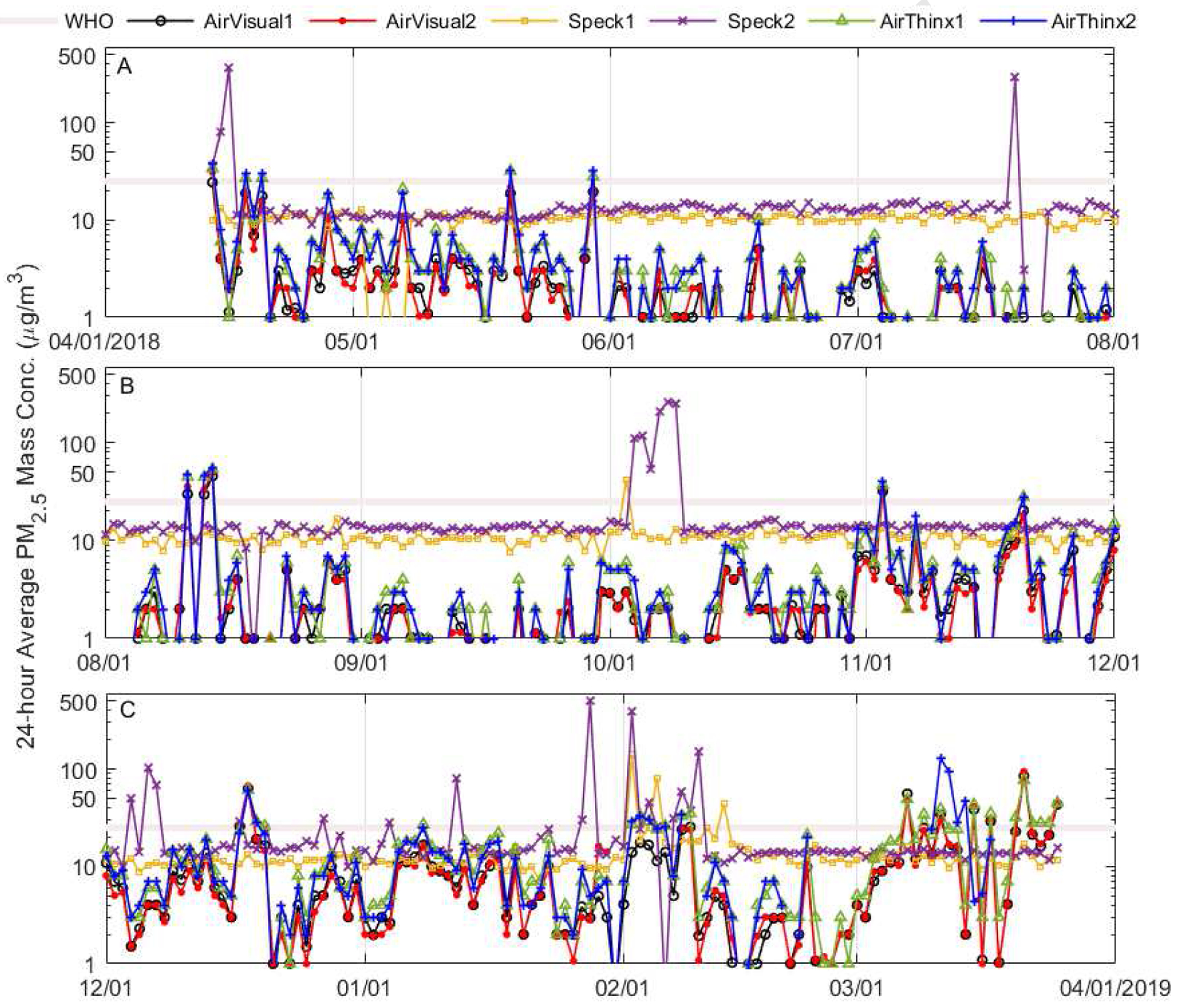
The 24-hour averaged measurements from April 13, 2018 through March 28, 2019 of the six units divided into four-month periods. The World Health Organization (WHO) 24-hour concentration guideline (25 μg/m3; solid horizontal line) is shown for reference. The concentrations are plotted on a log scale. The AirVisual Pro units are shown in black (open circle) and red (closed circle) lines. The Speck units are shown in yellow (square) and purple (X) lines. The AirThinx are shown in green (triangle) and blue (+) lines.
Table 2.
Summary of the 1-minute average PM2.5 mass concentrations (μg/m3), standard deviation (SD), median, coefficient of variation (CV), precision, correlation coefficients (R2) between units, and amount of missing data. Only measurement days without missing data were included in the calculations (n = 317 days).
| AirVisual Pro | Speck | AirThinx | |
|---|---|---|---|
| Unit 2 | 6.01 ± 21.92 | 23.42 ± 46.80 | 8.22 ± 22.54 |
| Unit 2 | 2.00 | 13.89 | 3.00 |
| Unit 2 | 3.65 | 2.00 | 2.74 |
| Precision | 0.11 | 0.69 | 0.12 |
| Unit-R2 | 0.99 | 0.17 | 0.99 |
Figure 2.

The raw (A, C) and filter-corrected (B, D) 1-minute averaged PM2.5 measurements from the six units and the pDR from two colocation periods. The AirVisual Pro units are shown in black (open circle) and red (closed circle) lines. The Speck units are shown in yellow (square) and purple (X) lines. The AirThinx are shown in green (triangle) and blue (+) lines. Each colocation period show was corrected using the corresponding filter (i.e., “individual”).
The corrected PM2.5 measurements from the six units and the pDR from two colocation periods are shown in Figure 2, and all colocation periods are shown in Supplemental Figure 2. Each colocation period was corrected using the corresponding filter (i.e., “individual”) in Figure 2. During the periods of colocation with the pDR, the average PM2.5 mass concentration from the two AirVisual Pro units were 5.11 and 5.03 μg/m3, compared to the Raw-pDR and pDR-corrected of 6.38 and 5.31 μg/m3, respectively (Table 3). The accuracies of the units compared with the pDR-corrected were 87.57 and 89.10%, which ranged between 61 and 99%, depending on the month. The lowest accuracies occurred when the mass concentrations were very low (e.g., the filter mass concentration was < 2 μg/m3 for the week), and the small differences (about 0.5 μg/m3) produced large percent errors. The RMSE for unit 1 and 2 were 0.59 and 0.64 μg/m3, respectively. Generally, the AirVisual Pros overestimated the mass concentration under about 10 μg/m3 and underestimated it at the higher concentrations (Figure 3B). A comparison of the AirVisual Pro/pDR-corrected as a function of RH and temperature did not reveal any large systematic errors due the environment (Supplemental Figure 5). The AirVisual Pro/pDR-corrected ratio was slightly higher (e.g., ~1.2) at RH > 70% compared to RH <40% (~1).
Table 3.
Summary of the 1-min averaged PM2.5 mass concentration (μg/m3), standard deviation (SD), coefficient of variation (CV), accuracy (%), root mean square error (RMSE), mean bias error (MBE), correlation coefficients (R2) for the 1-min averaged PM2.5 mass concentrations measured by the monitors compared with the pDR-corrected (filter corrected pDR-Raw measurements) and between units, and the precision. Only measurement days without missing data during the colocation periods were included in the calculations (n = 56 days). The temperature and RH from each unit are also shown. The data divided into four-month periods can be found in Supplemental Table 1.
| AirVisual 2 |
Speck 2 |
AirThinx 2 |
pDR- Corrected |
||||
|---|---|---|---|---|---|---|---|
|
PM2.5 (μg/m3) |
5.03 | 22.68 | 7.57 | 5.31 | |||
|
SD (μg/m3) |
10.24 | 20.96 | 11.34 | 13.07 | |||
| CV | 2.08 | 0.58 | 1.59 | 2.37 | |||
| Accuracy (%) | 85.61 | −405.73 | 39.89 | ||||
| RMSE | 0.64 | 17.37 | 2.26 | ||||
| MBE (%) | 3.45 | 505.73 | 60.11 | ||||
| pDR-R2 | 0.90 | 0.27 | 0.93 | ||||
| Unit-R2 | 0.99 | 0.19 | 1.00 | ||||
| Precision | 0.07 | 0.36 | 0.03 | ||||
| T (°C) | 21.61 | 20.95 | 22.73 | ||||
| RH (%) | 55.20 | 45.29 | 42.28 | ||||
Figure 3.
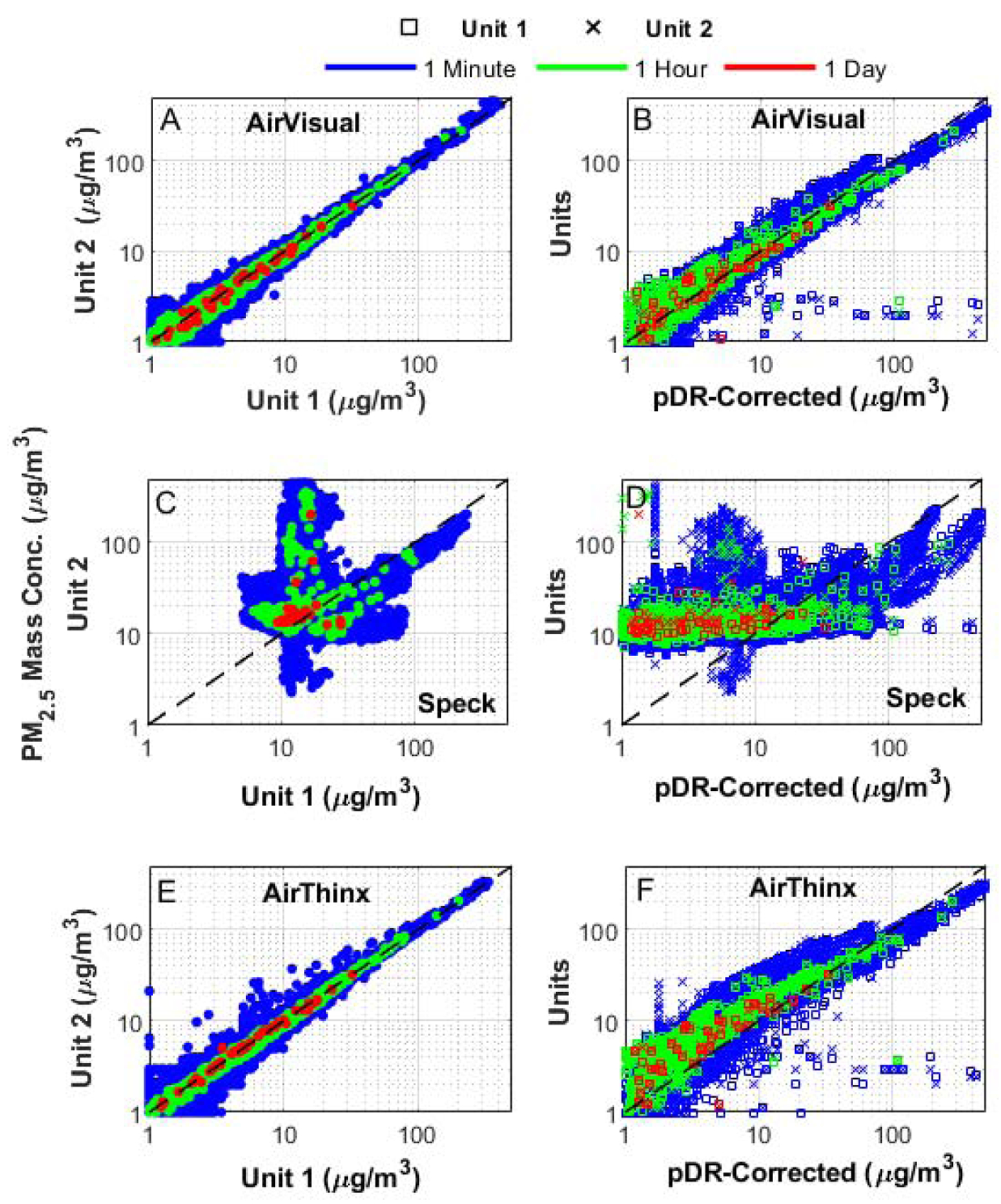
Scatterplots of the 1-minute (blue), 1-hour (green), and 24-hour (red) PM2.5 averages between the two units of each monitor type (A, C, and E) and between the monitors and the pDR-corrected (B, D, and F). Only measurement days without missing data during the colocation periods were included in the calculations (n = 56 days).
The overall pDR-R2 between the pDR-corrected and the AirVisual Pro units were about 0.90. The pDR-R2 did not exhibit any significant differences between measurements collected during the first four months compared to the last four months (Table 4; Supplemental Figure 4). If the data were averaged up to 1-hour or 24-hours, the pDR-R2 would be about 0.96 and 0.98, respectively (Figure 3; Table 4).
Table 4.
A) The 1-minute pDR-R2 divided into three periods: April – July (measurement months 1–4), xÀugust – November (5–8), and December – March (9–12). *The AirThinx unit 2 was offline during the final calibration period so the statistics only reflect the colocations during months 9–11. B-C) Comparisons of how using 1-minute, 1-hour, and 24-hour PM2.5 averages (μg/m3) effects the correlation coefficient (pDR-R2) and the accuracy of the Air Quality Index (AQI) category between the units and the pDR-corrected. Only measurement days without missing data during the colocation periods were included in the calculations (n = 56 days).
| A) pDR-R2 | Months 1–4 |
Months 5–8 |
Months 9 –12 |
|---|---|---|---|
| AirVisual 1 | 0.96 | 0.99 | 0.94 |
| AirVisual 2 | 0.98 | 0.99 | 0.94 |
| Speck 1 | 0.28 | 0.52 | 0.59 |
| Speck 2 | 0.53 | 0.50 | −0.01 |
| AirThinx 1 | 0.95 | 0.88 | 0.95 |
| AirThinx 2 | 0.96 | 0.88 | 0.94* |
| B) pDR-R2 | 1-Minute | 1-Hour | 1-Day |
| AirVisual 1 | 0.92 | 0.96 | 0.97 |
| AirVisual 2 | 0.92 | 0.96 | 0.97 |
| Speck 1 | 0.50 | 0.56 | 0.22 |
| Speck 2 | 0.27 | 0.30 | −0.08 |
| AirThinx 1 | 0.92 | 0.93 | 0.92 |
| AirThinx 2 | 0.93 | 0.94 | 0.91 |
| C) AQI Accuracy (%) | 1-Minute | 1-Hour | 1-Day |
| AirVisual 1 | 97 | 97 | 89 |
| AirVisual 2 | 98 | 98 | 89 |
| Speck 1 | 65 | 67 | 66 |
| Speck 2 | 14 | 13 | 16 |
| AirThinx 1 | 87 | 87 | 88 |
| AirThinx 2 | 87 | 86 | 88 |
b. Speck
The Speck exhibited a much lower precision between units (precision = 0.36, R2 = 0.19) with less consistent averages (13.54 vs 23.42 μg/m3), medians (11.28 vs 13.89), SDs (17.30 vs 46.80), and CVs (1.28 vs 2.00) between units. The Speck PM2.5 mass concentration did not exhibit diurnal trends similar to the other monitors. The Specks did show increasing concentrations during some of the cooking episodes (e.g., July 5 evening), but not all of them (e.g., July 1 evening). There were other times when they indicated a greater peak increase then the other instruments (e.g., July 3 morning). The Speck appears to have higher baseline values since 97% of the 1-min averages were above 8 μg/m3, compared to 17% for the AirVisual Pro. The Speck did not have any missing data, but there were periods of days when the units appeared to cycle between high values and low values about every ten minutes (Figure 2C). During these periods, the other units exhibited a typical diurnal cycle. If the unit was unplugged for several hours, the instrument would return to the typical values. There were no consistent factors present during the variable periods to explain the issue. The unit-R2 decreased as the year progressed since these erratic periods became more frequent and they rarely occurred at the same time between units (Figure 3C). If periods of time when the Speck measurements were at least an order of magnitude higher than the other monitors were excluded, the amount of missing time would be 20 days for Unit 1 and 22 days for Unit 2. The Speck reported temperatures between 14 and 23 °C, and the RH ranged between about 35 and 70%.
During the periods of colocation with the pDR, the average 1-minute PM2.5 mass concentration from the Speck units were 13.58 and 22.68 μg/m3 (Table 3). The overall accuracies of the units were −174.67 and −405.73% compared with the pDR-corrected. The accuracies are negative because the Speck concentrations were substantially larger than the pDR-corrected. The RMSE was 8.27 and 17.37 μg/m3 for unit 1 and 2, respectively, and the MBE was 274.67 and 505.73% for unit 1 and 2, respectively. The pDR-R2 were noticeably different at 0.50 and 0.27, and they did not display a consistent trend throughout the year (Table 4). For example, the pDR-R2 for unit 1 was −0.16 during month 4 and 0.78 during month 7. Changing the averaging interval did not increase the correlation between the two types of instruments (Figure 3; Table 4). It is possible that the Speck sensor would be accurate in a more polluted environment since they appear to have relatively high baseline values. The Speck pDR-R2 from the times when the mass concentration was greater than 10 μg/m3 was about 0.6.
A comparison of the Speck/pDR-Corrected did not reveal any systematic biases as a function of temperature, but the Speck generally overestimated the PM2.5 mass concentration more during periods of higher RH (Supplemental Figure 5). For example, the Speck/pDR-Corrected ratio was about 2 at 40% RH and about 5.5 for 70% RH.
c. AirThinx
The AirThinx exhibited a precision of 0.12 and a unit-R2 of 0.99, with similar average (8.20 vs 8.22 μg/m3), median (3.00 vs 3.00), SD (21.05 vs 22.54), and CV (2.57 vs 2.74) values. The AirThinx measurements exhibited a reasonable trend with peak concentrations occurring during periods of cooking and the lowest concentrations occurring overnight (Figure 2A). The peak values were generally higher during the cooking periods than the other monitors. The precision between units remained consistent throughout the year with a precision of 0.07 at beginning of the measurement period and of 0.1 at the end, and the R2 remained greater than 0.90 for all months (Supplemental Table 1). Near the end of the measurement period, the micro-usb port became loose on one unit and the power cord would not connect appropriately resulting in 9% data loss. The AirThinx reported temperatures between 18 and 25 °C, and the RH ranged between about 20 and 80%.
During the periods of colocation with the pDR, the average PM2.5 mass concentration from the AirThinx were 7.56 and 7.57 μg/m3. The accuracies of the units compared with the pDR-corrected were 42.32 and 39.89%, and the highest and lowest accuracies for a given month were 89 and −36%. The RMSE was 2.25 and 2.26 μg/m3 for unit 1 and 2, respectively, and the MBE was 57.68 and 60.11% for unit 1 and 2, respectively. The AirThinx exhibited the lowest accuracy during the cleanest month (pDR-corrected = 1.83 μg/m3; unit concentrations = 4.21 and 4.33 μg/m3), but the correlation was high (pDR-R2 = 0.98). The average pDR-R2 was about 0.92, but the pDR-R2 remained above 0.87 for all months and the greatest pDR-R2 from a colocation period was 0.98. Changing the averaging interval did not significantly affect the pDR-R2 correlation (Figure 3; Table 4). Overall, the AirThinx overestimated the mass concentration for measured concentrations under about 50 μg/m3 and underestimated it at the higher concentrations (Figure 3F). The AirThinx appears to exhibit a small dependency on the RH and temperature, with the greatest AirThinx/pDR-corrected ratios occurring at lower temperatures (< 22 °C) and higher RHs (Supplemental Figure 4). These environmental factors both occurred during the summer months, so the observed trend may be due to a PM seasonal composition factor rather than temperature or RH biases.
d. Air Quality Index
Since all the monitors provide a visual indicator about the air quality in the room, we wanted to analyze how often a participant would see the various AQI levels since this would likely affect how a person perceives the indoor air quality of the residence and to evaluate the reported AQI accuracy. Even though the AQI was designed to be applied to ambient air pollution, this metric is frequently utilized for indoor air quality measurement by this type of monitor because there are no regulatory standards for a non-occupational setting. In Figure 4, the 1-minute averaged PM2.5 mass concentrations have been divided into the corresponding AQI bins. The values for each monitor from the full and colocation periods are shown in supplemental Table 2, and a bar graph of the six monitors’ AQI from the full measurement period can be found in Supplemental Figure 6. If the pDR had a method of displaying the AQI, it would have a exhibited “good” AQI 85.6% of the time, a “moderate” AQI 10.6% of the time, a “unhealthy for sensitive groups” AQI 1.4% of the time, a “unhealthy” AQI 2.1% of the time, a “very unhealthy” AQI 0.3% of the time, and a “hazardous” AQI 0.08% of the time. Overall, the 1-minute pDR-corrected AQI bin averages matched the AirVisual Pro, Speck, and AirThinx bins about 97, 40, and 87% of the time (Table 4). The largest difference for units of the same type was “good” and “moderate” Speck measurements. This was particularly noticeable during the colocation measurements; unit 1 reported “good” values 63.1% of the time compared to unit 2 with 6.5%. This is likely because baseline concentrations differed by few μg/m3 (around 10 vs 14 μg/m3 for units 1 and 2, respectively) resulting in one unit reporting values above the “good” cutoff while the other reported values below the AQI threshold.
Figure 4.
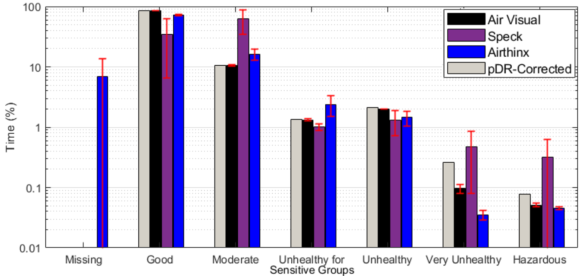
A comparison of the 1-minute averaged PM2.5 mass concentrations binned based on Air Quality Index (AQI) levels (n = 75 days). The error bars indicate the range between the two units. The AQI was defined as follow: good = 0 – 12 μg/m3, moderate = 12.1 – 35.4 μg/m3, unhealthy for sensitive groups= 35.5 – 55.4 μg/m3, unhealthy = 55.5 – 150.4 μg/m3, very unhealthy = 150.5 – 250.4 μg/m3, and hazardous > 250.4 μg/m3. Only measurements collected during the colocation periods were included. The percent of time is shown on a log scale.
e. Corrections Factors
Scatterplots of the pDR-corrected PM2.5 measurements against the one unit from each type of monitors (“unit 1”) is shown in Figure 5. For all monitors, the scenario in which the monitors were monthly calibrated (i.e., individual) yielded the highest accuracies (>96%). The “average” correction increased the accuracy for all the monitors, but the magnitude of the increased accuracy depended on the type of monitor. The AirVisual Pro only increased nominally (<2%), but the Speck and AirThinx increased by much larger percentages (about 211 % and 41%, respectively). The first and last month scenarios yielded mixed results. For the AirVisual Pro, using the first and last month’s correction factors did not significantly change the resultant accuracy since the AirVisual Pro was generally similar to the pDR-corrected. Using the first month’s data to correct the Speck’s full data set resulted in a majority of the points underestimating the true mass concentrations and using the last month’s data resulted in a majority of the points overestimating the mass concentration. Using the correction factor from just one month yielded accuracies for the AirThinx in the 60–80% range (RMSE < 1.5 μg/m3).
Figure 5.

Scatterplots of the 1-minute averaged pDR-corrected PM2.5 measurements against the monitor measurements that have been filter corrected under different scenarios. “First Month” indicates that all of the colocated measurement periods were corrected using the filter data collected during the first month (blue square); representing a scenario that the monitors were only calibrated during the first week of deployment. “Last Month” indicated that all of the colocated measurements were corrected using the filter data collected during the last month (red circle); a scenario that reflect the accuracy if the monitors were only calibrated during the at the end of a deployment. “Individual” means that each month’s data was calibrated by the corresponding filter (black X). “Average” means the correction factor was generated by taking an average of all the filter data and applying it to the full measurement period (yellow filled circle). The axes are shown on a log scale.
4. Discussion
This study evaluated performance of the monitor packages, not the just component sensors, in order to assess the sensors, the built-in calibration system, and the need for additional data to achieve high accuracy over long duration deployments. Ultimately, the level of accuracy needed for a specific research question determines the amount of additional measurements required. The AirVisual Pro exhibited an accuracy of about 86% without any adjustments, so it may be reasonable to use only one or no filter measurements based on the known information about the residence and accuracy requirements for the application. The AirThinx exhibited much lower accuracy, but a consistent bias. It may be feasible to address known instrumental biases after the sampling period has been completed. For example, since the AirThinx units consistently overestimated the mass concentration under about 50 μg/m3 and underestimated it at the higher concentrations (Figure 3F), it is likely that a user could utilize a simple quadratic equation during post-processing to obtain more accurate results. By using Equation 7, which is simply derived from the quadratic fit of AirThinx vs pDR-corrected, the resultant accuracy would be 87% without any filter correction.
| Equation 7 |
Since the AirVisual Pro and AirThinx do not exhibit strong RH correlations, it is likely that the monitors account for environmental factors to some degree, which may simplify post processing. It is also possible that a research question could be adequately addressed by using the AQI classification instead of the true mass concentration. For our study, the 1-minute AirVisual Pro, Speck, and AirThinx AQI bins were correct about 97, 40, and 87% of the time, respectively, which is markedly better than the accuracy.
It is important to note that using a simple filter correction factor is convenient, but it may not be useful in all scenarios since it is derived from taking the PM2.5 measured by a monitor over a long period of time (here about a week) and comparing it to the filter mass concentration. Also, this study was conducted in a relatively clean, nonsmoking home, so their accuracy in homes with much higher PM loadings is unknown.
It is critical to know the strengths and limitations of available monitors in order to select the best monitor for the sampling environment. After synthesizing the available information from our study and previously reported results, the uncorrected AirVisual Pro data would likely exhibit the highest accuracy when used in nonsmoking indoor environments and only moderate correlations if used in outdoor ambient settings.[14, 22, 32, 35] The synthesized AirThinx data suggests that it can obtain meaningful data indoors and outdoors, but the data will need validated data sources to achieve high accuracy.[34] The PM2.5 sensor included in the AirThinx (Plantower) has been thoroughly investigated in ambient and laboratory settings, with generally positive findings.[28, 29] The Speck has not exhibited accurate data in most indoor or outdoor settings, with the exception of samples dominated by dust.[30, 36][4][14]
5. Conclusions
We evaluated the accuracy and precision of three monitor types (AirVisual Pro, Speck, and AirThinx) over a one-year period in a residential setting. The monitors collected data continuously in the living room, and a reference instrument (pDR) with-time resolved and filter-based measurements was operated for about a week each month. The AirVisual Pro exhibited high accuracy, high pDR-R2 correlations, good precision between units, minimal dependence on temperature and RH, and minimal drift over the year period. The AirThinx exhibited excellent precision, high pDR-R2 values, minimal dependence on temperature and RH, and minimal drift over the year period. However, the AirThinx required filter colocations and/or post processing to achieve high accuracies. We assessed the correlation between the reference instrument and the monitors as a function of time (over months) and averaging interval. Both instruments exhibited high R2 values at the beginning and end of the measurement year, and both exhibited high R2 values when averaged in 1-minute, 1-hour, and 24-hour intervals. Overall, the characteristics of these two monitors makes them potentially useful for high quality residential exposure assessments. The Speck was not able to produce useable data in this study because a large portion of the measured concentrations were below the high baseline concentration reported by the device, resulting in most household concentrations below the level of the noise in the data. It is clear that low-cost monitors can be useful for indoor exposure assessments, but data quality varies dramatically by brand and an evaluation of each monitor is essential. Future work should include extended measurements in a residence with smoking, candles, or fireplace sources, since these activities may produce a higher PM concentrations than commonly observed in this study, and it would be beneficial to observe the response of the sensors to persistent high PM loadings.
Supplementary Material
Highlights.
We evaluated three monitors (AirVisual Pro, Speck, and AirThinx) over 12-months.
The AirVisual Pro exhibited the best accuracy compared to the filter at about 86%.
The AirThinx exhibited the highest precision between units (R2 = 0.99).
Low-cost monitor shows exciting potential for use in scientific research.
6. Acknowledgment
This publication was developed under Assistance Agreement no. RD835871 awarded by the U.S. Environmental Protection Agency to Yale University. It has not been formally reviewed by the Environmental Protection Agency (EPA). The views expressed in this document are solely those of the authors and do not necessarily reflect those of the Agency. The EPA does not endorse any products or commercial services mentioned in this publication. The research reported in this publication was also supported by the National Institute of Environmental Health Sciences of the National Institutes of Health under awards number 1K23ES029985-01 and K99ES029116. The content is solely the responsibility of the authors and does not necessarily represent the official views of the National Institutes of Health.
Footnotes
Publisher's Disclaimer: This is a PDF file of an unedited manuscript that has been accepted for publication. As a service to our customers we are providing this early version of the manuscript. The manuscript will undergo copyediting, typesetting, and review of the resulting proof before it is published in its final form. Please note that during the production process errors may be discovered which could affect the content, and all legal disclaimers that apply to the journal pertain.
Supporting Information.
Supplemental Figures (PDF)
Declaration of interests
The authors declare that they have no known competing financial interests or personal relationships that could have appeared to influence the work reported in this paper.
The authors declare the following financial interests/personal relationships which may be considered as potential competing interests:
REFERENCES
- 1.Anderson JO, Thundiyil JG, and Stolbach A, Clearing the air: a review of the effects of particulate matter air pollution on human health. J Med Toxicol, 2012. 8(2): p. 166–75. [DOI] [PMC free article] [PubMed] [Google Scholar]
- 2.Organization WH, Global Health Estimates 2016: Deaths by cause, age, sex, by country and by region, 2000–2016. 2018. [Google Scholar]
- 3.Dockery DW, et al. , An association between air pollution and mortality in six U.S. cities. N Engl J Med, 1993. 329(24): p. 1753–9. [DOI] [PubMed] [Google Scholar]
- 4.Zamora ML, et al. , Maternal exposure to PM 2.5 in south Texas, a pilot study. Science of The Total Environment, 2018. 628: p. 1497–1507. [DOI] [PubMed] [Google Scholar]
- 5.Braniš M and Kolomazníková J, Monitoring of long-term personal exposure to fine particulate matter (PM 2.5). Air Quality, Atmosphere & Health, 2010. 3(4): p. 235–243. [Google Scholar]
- 6.Weisel CP, et al. , Relationship of Indoor, Outdoor and Personal Air (RIOPA) study: study design, methods and quality assurance/control results. Journal of Exposure Science and Environmental Epidemiology, 2005. 15(2): p. 123. [DOI] [PubMed] [Google Scholar]
- 7.Buonanno G, et al. , INDIVIDUAL EXPOSURE OF WOMEN TO FINE AND COARSE PM. Environmental Engineering & Management Journal (EEMJ), 2015. 14(4). [Google Scholar]
- 8.Adgate JL, et al. , Spatial and temporal variability in outdoor, indoor, and personal PM2. 5 exposure. Atmospheric Environment, 2002. 36(20): p. 3255–3265. [Google Scholar]
- 9.Klepeis NE, et al. , The National Human Activity Pattern Survey (NHAPS): a resource for assessing exposure to environmental pollutants. Journal of Exposure Science and Environmental Epidemiology, 2001. 11(3): p. 231. [DOI] [PubMed] [Google Scholar]
- 10.Buonanno G, Morawska L, and Stabile L, Particle emission factors during cooking activities. Atmospheric Environment, 2009. 43(20): p. 3235–3242. [Google Scholar]
- 11.Madureira J, et al. , Indoor air quality in Portuguese schools: levels and sources of pollutants. Indoor air, 2016. 26(4): p. 526–537. [DOI] [PubMed] [Google Scholar]
- 12.Meng QY, et al. , Determinants of indoor and personal exposure to PM2. 5 of indoor and outdoor origin during the RIOPA study. Atmospheric Environment, 2009. 43(36): p. 5750–5758. [DOI] [PMC free article] [PubMed] [Google Scholar]
- 13.Singer BC, et al. , Indoor secondary pollutants from cleaning product and air freshener use in the presence of ozone. Atmospheric Environment, 2006. 40(35): p. 6696–6710. [Google Scholar]
- 14.Singer BC and Delp WW, Response of consumer and research grade indoor air quality monitors to residential sources of fine particles. Indoor Air, 2018. 28(4): p. 624–639. [DOI] [PubMed] [Google Scholar]
- 15.Graney JR, Landis MS, and Norris GA, Concentrations and solubility of metals from indoor and personal exposure PM2. 5 samples. Atmospheric Environment, 2004. 38(2): p. 237–247. [Google Scholar]
- 16.Long CM, Suh HH, and Koutrakis P, Characterization of indoor particle sources using continuous mass and size monitors. Journal of the Air & Waste Management Association, 2000. 50(7): p. 1236–1250. [DOI] [PubMed] [Google Scholar]
- 17.Massey D, et al. , Indoor/outdoor relationship of fine particles less than 2.5 μm (PM2. 5) in residential homes locations in central Indian region. Building and Environment, 2009. 44(10): p. 2037–2045. [Google Scholar]
- 18.Duan C, et al. , Residential Exposure to PM2. 5 and Ozone and Progression of Subclinical Atherosclerosis Among Women Transitioning Through Menopause: The Study of Women’s Health Across the Nation. Journal of Women’s Health, 2019. [DOI] [PMC free article] [PubMed] [Google Scholar]
- 19.Hoffmann B, et al. , Residential exposure to traffic is associated with coronary atherosclerosis. Circulation, 2007. 116(5): p. 489–496. [DOI] [PubMed] [Google Scholar]
- 20.Hvidtfeldt UA, et al. , Long-term residential exposure to PM2. 5, PM10, black carbon, NO2, and ozone and mortality in a Danish cohort. Environment international, 2019. 123: p. 265–272. [DOI] [PubMed] [Google Scholar]
- 21.Hystad P, et al. , Long-term residential exposure to air pollution and lung cancer risk. Epidemiology, 2013: p. 762–772. [DOI] [PubMed] [Google Scholar]
- 22.Tan B, Laboratory Evaluation of Low to Medium Cost Particle Sensors. 2017, University of Waterloo. [Google Scholar]
- 23.Ikram J, et al. , View: implementing low cost air quality monitoring solution for urban areas. Sensors, 2012. 4: p. 100. [Google Scholar]
- 24.Mead MI, et al. , The use of electrochemical sensors for monitoring urban air quality in low-cost, high-density networks. Atmospheric Environment, 2013. 70: p. 186–203. [Google Scholar]
- 25.Sousan S, et al. , Inter-comparison of low-cost sensors for measuring the mass concentration of occupational aerosols. Aerosol Science and Technology, 2016. 50(5): p. 462–473. [DOI] [PMC free article] [PubMed] [Google Scholar]
- 26.Clements AL, et al. , Low-cost air quality monitoring tools: from research to practice (a workshop summary). Sensors, 2017. 17(11): p. 2478. [DOI] [PMC free article] [PubMed] [Google Scholar]
- 27.Hagler GS, et al. , Air Quality Sensors and Data Adjustment Algorithms: When Is It No Longer a Measurement? 2018, ACS Publications. [DOI] [PMC free article] [PubMed] [Google Scholar]
- 28.Levy Zamora M, et al. , Field and laboratory evaluations of the low-cost plantower particulate matter sensor. Environmental science & technology, 2018. 53(2): p. 838–849. [DOI] [PubMed] [Google Scholar]
- 29.Kelly K, et al. , Ambient and laboratory evaluation of a low-cost particulate matter sensor. Environmental Pollution, 2017. 221: p. 491–500. [DOI] [PMC free article] [PubMed] [Google Scholar]
- 30.Sousan S, et al. , Evaluation of consumer monitors to measure particulate matter. J Aerosol Sci, 2017. 107: p. 123–133. [DOI] [PMC free article] [PubMed] [Google Scholar]
- 31.Sousan S, et al. , Inter-comparison of Low-cost Sensors for Measuring the Mass Concentration of Occupational Aerosols. Aerosol Sci Technol, 2016. 50(5): p. 462–473. [DOI] [PMC free article] [PubMed] [Google Scholar]
- 32.Feenstra B, et al. , Performance evaluation of twelve low-cost PM2. 5 sensors at an ambient air monitoring site. Atmospheric Environment, 2019. 216: p. 116946. [Google Scholar]
- 33.Manikonda A, et al. , Laboratory assessment of low-cost PM monitors. Journal of Aerosol Science, 2016. 102: p. 29–40. [Google Scholar]
- 34.(AQ-SPEC), A.Q.S.P.E.C. Field Evaluation of AirThinx IAQ. 2018; Available from: http://www.aqmd.gov/docs/default-source/aq-spec/field-evaluations/airthinx-iaq--field-evaluation.pdf?sfvrsn=18.
- 35.(AQ-SPEC), A.Q.S.P.E.C. Field Evaluation IQAir AirVisual Pro (v1.1683) Sensor. 2018; Available from: http://www.aqmd.gov/docs/default-source/aq-spec/field-evaluations/iqair-airvisual-pro-(fw1-1683)---field-evaluation.pdf?sfvrsn=8.
- 36.(AQ-SPEC), A.Q.S.P.E.C. Field Evaluation Speck Sensor. 2015; Available from: http://www.aqmd.gov/docs/default-source/aq-spec/field-evaluations/speck-sensor---field-evaluation.pdf?sfvrsn=4.
- 37.IQAir. AirVisual Pro Tech Spec. CD1092.3_INT_171227 2019. [cited 2019 10/22/2019]; Available from: https://www.iqair.com/support/tech-specs/airvisual-pro.
- 38.NEWFITNESSGADGETS.COM. Check the Air Quality around you with AirVisual Node! 2017. November 20, 2017 10/25/2019]; Available from: https://newfitnessgadgets.com/airvisual-node.
- 39.Inc., A. Speck FAQ. 10/25/2019]; Available from: https://www.specksensor.com/support/faq.
- 40.Inc., A. Speck Technical Specifications. 10/25/2019]; Available from: https://www.specksensor.com/support/tech-specs.
- 41.Airthinx. Airthinx Tech Spec. 2018. 10/25/2019]; Available from: https://airthinx.io/images/brochures/airthinx_device-864278a2c4.pdf.
- 42.Levy Zamora M, et al. , Field and Laboratory Evaluations of the low-cost Plantower Particulate Matter Sensor. Environment International, under review. [DOI] [PubMed] [Google Scholar]
- 43.Laulainen N, Summary of conclusions and recommendations from a visibility science workshop, in Technical Basis and Issues for a National Assessment for Visibility Impairment. 1993, Prepared for US DOE, Pacific Northwest Lab, Richland, WA (United States). [Google Scholar]
- 44.Soneja S, et al. , Humidity and gravimetric equivalency adjustments for nephelometer-based particulate matter measurements of emissions from solid biomass fuel use in cookstoves. International journal of environmental research and public health, 2014. 11(6): p. 6400–6416. [DOI] [PMC free article] [PubMed] [Google Scholar]
- 45.Chakrabarti B, et al. , Performance evaluation of the active-flow personal DataRAM PM2.5 mass monitor (Thermo Anderson pDR-1200) designed for continuous personal exposure measurements. Atmospheric Environment, 2004. 38: p. 3329–3340. [Google Scholar]
- 46.Wallace LA, et al. , Validation of continuous particle monitors for personal, indoor, and outdoor exposures. Journal of exposure science & environmental epidemiology, 2011. 21(1): p. 49–64. [DOI] [PubMed] [Google Scholar]
- 47.Wang Z, et al. , Comparison of real-time instruments and gravimetric method when measuring particulate matter in a residential building. Journal of the Air & Waste Management Association (1995), 2016. 66(11): p. 1109–1120. [DOI] [PMC free article] [PubMed] [Google Scholar]
Associated Data
This section collects any data citations, data availability statements, or supplementary materials included in this article.