Boosting the accuracy of protein secondary structure prediction through nearest neighbor search and method hybridization

Abstract

Motivation

Protein secondary structure prediction is a fundamental precursor to many bioinformatics tasks. Nearly all state-of-the-art tools when computing their secondary structure prediction do not explicitly leverage the vast number of proteins whose structure is known. Leveraging this additional information in a so-called template-based method has the potential to significantly boost prediction accuracy.

Method

We present a new hybrid approach to secondary structure prediction that gains the advantages of both template- and non-template-based methods. Our core template-based method is an algorithmic approach that uses metric-space nearest neighbor search over a template database of fixed-length amino acid words to determine estimated class-membership probabilities for each residue in the protein. These probabilities are then input to a dynamic programming algorithm that finds a physically valid maximum-likelihood prediction for the entire protein. Our hybrid approach exploits a novel accuracy estimator for our core method, which estimates the unknown true accuracy of its prediction, to discern when to switch between template- and non-template-based methods.

Results

On challenging CASP benchmarks, the resulting hybrid approach boosts the state-of-the-art Q₈ accuracy by more than 2–10%, and Q₃ accuracy by more than 1–3%, yielding the most accurate method currently available for both 3- and 8-state secondary structure prediction.

Availability and implementation

A preliminary implementation in a new tool we call Nnessy is available free for non-commercial use at http://nnessy.cs.arizona.edu.

1 Introduction

Predicting the secondary structure of a protein from its amino acid sequence is a classic and fundamental problem in bioinformatics, that is a building block in many tasks such as protein tertiary structure prediction (Dill and MacCallum, 2012), protein multiple sequence alignment (Deng and Cheng, 2011; Kececioglu et al., 2010; Lu and Sze, 2008) and solvent accessibility prediction (Adamczak et al., 2004). The true secondary structure of a protein is usually obtained from its known tertiary structure using a tool such as DSSP (Kabsch and Sander, 1983), which labels the amino acid residues in the protein (based on the torsion angles of their backbone) with eight states, that are traditionally reduced to just three classes: G ($3_{10}$-helix), H (α-helix) and I (π-helix), are usually classified as alpha (α); B (isolated bridge) and E (extended sheet) are usually classified as beta (β); and everything else is usually classified as coil (γ), representing ‘other’ (or the unstructured class).

State-of-the-art tools for secondary structure prediction perform sequence database homology searches over proteins with unknown structure, using PSI-BLAST (Altschul et al., 1997) or a similar search tool, to generate a position-specific scoring matrix across the residues of the protein. Most tools do not take advantage of the vast number of proteins with known structure.

In contrast, our core approach instead uses a variant of k-nearest neighbor classification over a template database of proteins with known structure to estimate secondary structure class membership probabilities, followed by a fast dynamic programming algorithm to compute a globally optimal maximum-likelihood secondary structure prediction.

Related work

A plethora of methods have been proposed for protein secondary structure prediction over the past 60 years. A recent survey paper (Yang et al., 2016) cites over 45 tools developed since 1960. Most recent tools use results from protein sequence database homology searches (Drozdetskiy et al., 2015; Jones, 1999; Ma et al., 2018), possibly combined with other information, such as physiochemical structural properties of the input sequence (Dor and Zhou, 2006), backbone torsion angles (Faraggi et al., 2012), as well as small databases of templates from proteins for which secondary structure is known (Li et al., 2012; Pollastri et al., 2002; Saraswathi et al., 2012). This additional information is then often fed into neural networks, such as filter neural networks (Mirabello and Pollastri, 2013; Yaseen and Li, 2014) or deep neural networks (Heffernan et al., 2015; Qi et al., 2012; Spencer et al., 2015; Wang et al., 2016), that output the structure prediction.

Currently, the most widely-used tools are perhaps PSIPRED (Jones, 1999) and JPRED (Drozdetskiy et al., 2015), which typically have an average Q₃ accuracy for 3-state secondary structure prediction on benchmark datasets of around 80–85%. Neither of these tools can predict 8-state secondary structure. PSIPRED was among the first tools to achieve improved accuracy through a PSI-BLAST search, and currently searches the UNIREF90 sequence database to obtain a sequence profile that is then fed into a two-stage neural network. JPRED incorporates both PSI-BLAST and HMMer (Finn et al., 2011) sequence profiles as inputs to their neural network.

The state-of-the-art tools that achieve the highest currently available accuracy include SSpro (Pollastri et al., 2002), DeepCNF (Wang et al., 2016), PORTER (Mirabello and Pollastri, 2013) and PSRSM (Ma et al., 2018), which on standard benchmarks typically achieve Q₃ accuracy around 85–90%. The state-of-the-art tools that predict 8-state secondary structure see a large drop in accuracy to around 72% Q₈ accuracy. SSpro is the only state-of-the-art tool that uses so-called template data, by searching for proteins of known secondary structure that share sequence homology with the query protein—if such proteins exist. For protein residues not covered by a matching template, SSpro uses a neural network to predict their structure class. This template-based method is very accurate when good matches can be found, but much less accurate when no good template exists (dropping around 10% in accuracy). DeepCNF and PORTER use variations on deep convolutional neural networks and conditional neural fields on sequence profiles. PSRSM uses semi-random subspaces, a variation on support vector machines.

Our contributions

In contrast to prior work, we present an algorithmic approach to protein secondary structure prediction. At a high level, our core method is template-based, and avoids sequence database homology searches to surpass the speed of state-of-the-art tools; our hybrid method then builds on this core approach, in combination with an alternate non-template-based method, to surpass the accuracy of the state-of-the-art. (SSpro, prior to our work, also combines a template- and non-template-based approach; our hybrid method is unique in that it can discern when to switch between such approaches by leveraging a novel accuracy estimator.) More concretely, this work makes the following contributions.

• Our core method replaces expensive protein sequence database homology search by nearest neighbor search over a smaller template database of fixed-length words under substitution distance, which is significantly faster, and has a large potential for further speedup.

• The core method finds a globally-optimal maximum likelihood prediction for the secondary structure of the entire protein, considering class membership probabilities at residues, structure transition probabilities between residues, and distributions of run lengths for structure classes. This maximum likelihood prediction is efficiently computed using dynamic programming.

• A unique aspect of our core approach is that it yields a novel accuracy estimator, that for the first time can quickly estimate the unknown true accuracy of its prediction. This estimate is respectively within roughly 5% and 8% on average of the unknown Q₃ and Q₈ accuracy for 3- and 8-state prediction.

• This new accuracy estimator leads to a natural hybrid method, which combines our core template-based approach with an alternate non-template-based method. The resulting hybrid gains the advantages of both: the high accuracy of our core approach when the protein has good matches to our template database, and the more stable accuracy of a non-template-based method in general. Remarkably, the average accuracy of this new hybrid method is always better than both of its base methods, across all standard benchmarks.

• The new core and hybrid methods afford a significant accuracy boost. On the challenging CASP benchmarks, where we predict on a CASP dataset using a template database constructed over proteins entered into PDB prior to the CASP competition date, our hybrid method boosts state-of-the-art Q₈ accuracy by more than 2–10%, and Q₃ accuracy by more than 1–3%. On yearly PDB datasets, where we predict on proteins entered into PDB in a given year using a template database over proteins from prior years, our core method boosts state-of-the-art Q₈ accuracy by more than 3%, and our hybrid method by more than 8–12%.

In short, our hybrid approach is the most accurate method currently available for both 3- and 8-state prediction on all standard benchmarks.

A preliminary implementation in a new tool we call Nnessy (short for ‘'nearest-neighbor-based prediction of protein secondary structure without searching for homology’') is available free for non-commercial use at http://nnessy.cs.arizona.edu.

Overview

The next section describes our approach, including the variant of nearest neighbor classification used by the core method for estimating class membership probabilities, the dynamic programming algorithm for maximum likelihood prediction, our accuracy estimator and the hybrid method. Section 3 presents experimental results comparing the 3- and 8-state prediction accuracy of our approach to other state-of-the-art tools. Section 4 studies the behavior of our approach to provide insight on why it performs well. Finally Section 5 concludes.

2 Methods

We first describe how our core approach, which is template-based, computes a secondary structure prediction, and then explain how we leverage it in a new hybrid approach that combines the advantages of both template- and non-template-based methods.

Our core approach proceeds in two phases. The first phase estimates for each residue in the protein its class membership probability for secondary structure classes. The second phase takes these probability estimates, together with empirical transition rates between secondary structure runs from different classes and empirical distributions of run lengths, and computes a secondary structure prediction for the entire protein that is globally optimal with respect to a maximum likelihood objective. The residue class membership probabilities for the first phase are estimated by a variant of nearest neighbor classification, using nearest neighbor search over fixed-length amino acid words. The optimal maximum likelihood prediction for the second phase is computed by dynamic programming.

Our hybrid approach exploits a unique aspect of this core method: that we can compute an estimated accuracy for its prediction. This accuracy estimate enables our hybrid method to recognize when our core template-based prediction may be inaccurate, and hence switch to a potentially more accurate non-template-based method.

2.1 Estimating structure probabilities at residues

Key to our core approach for secondary structure prediction is estimating class membership probabilities for the residues of the protein: at each position i in the protein, for each structure class c, the probability that class c is the true secondary structure state of the residue at position i. We estimate these probabilities by a form of nearest neighbor classification, using words of a fixed length $\ell$ extracted from the amino acid sequence P of the protein.

Given a collection of proteins with known tertiary structure, and hence whose correct secondary structure is known, we form a template database D by extracting all words of length $\ell$ from their amino acid sequences, together with their associated secondary structure word of the same length. (If the same amino acid word w occurs more than once in the protein collection with different associated secondary structure words, we collapse the differences into a single secondary structure word over an extended secondary structure alphabet that contains ambiguity codes for non-empty subsets of the structure classes. For each amino acid word in database D, we also keep a count of its number of occurrences in the protein collection. If the amino acid sequence for the protein has positions with ambiguous amino acids, we retain these ambiguities in the amino acid word put into D.)

To predict the secondary structure of a new protein, we extract words of this length $\ell$ from its amino acid sequence P, and for each such query word w from P, we find its so-called k-nearest neighbors in template database D: the k amino acid words v in D that have smallest distance d(v, w) to query word w, under a word distance function d.

The associated secondary structure words in D for these k-nearest neighbors of w are then used to estimate class membership probabilities. For a given residue at position i in P, there are, in general, $\ell$ words of length $\ell$ that overlap position i. For each of these $\ell$ query words w overlapping i, we find their k-nearest neighbors v in D, and combine together the associated secondary structure words for all of these $k\ell$ overlapping words v to estimate the class membership probabilities for residue i.

We next describe how we measure word distances, search for nearest neighbors, and combine overlapping words into a probability estimate.

2.1.1 Measuring distances between words

To measure the distance d between two amino acid words v and w, both of length $\ell$, we use a form of substitution distance, $d(v,w) = \sum _{1\le i\le \ell } \delta \left(v\right[i],w[i\left]\right)$, where $\delta (a,b)$ is the substitution dissimilarity score for amino acid pair a, b. For substitution scores δ, we take the standard VTML200 amino acid similarity matrix (Müller et al., 2002) and transform it into dissimilarity scores by negating its values, shifting them to positive scores by adding in the most negative value, and rescaling them into the range $[0,1]$.

2.1.2 Finding nearest neighbors

When the substitution scores δ in word distance function d satisfy the so-called triangle inequality, namely $\delta (a,c)\le \delta (a,b)+\delta (b,c)$ for all amino acids a, b, c, word distance d will also satisfy the triangle inequality $d(u,w)\le d(u,v)+d(v,w)$ for all words u, v, w. The transformed VTML dissimilarity scores δ mentioned above do satisfy the triangle inequality, hence word distance function d does as well.

In general, a distance function d that satisfies the triangle inequality, non-negativity ($d(v,w)\ge 0$ for all v, w), symmetry ($d(v,w)=d(w,v)$ for all v, w) and identity ($d(v,w)=0$ iff v = w), is called a metric. When word distance function d is a metric, template database D under distance d is known as a metric space.

One of the best data structures for nearest neighbor search in a metric space is the cover tree of Beygelzimer et al. (2006). Theoretically, cover trees permit nearest neighbor searches over a set of n objects in $O(\text{log}\hspace{0.17em}n)$ time, after constructing a cover tree in $O(n\hspace{0.17em}\text{log}\hspace{0.17em}n)$ time, assuming the intrinsic dimension of the metric space has a so-called bounded expansion constant (Beygelzimer et al., 2006). (For actual data, the expansion constant can be exponential in the intrinsic dimension.) In our implementation, for nearest neighbor search we use the recently developed dispersion tree data structure of Woerner and Kececioglu, which in extensive testing on scientific data is significantly faster in practice than cover trees (Woerner, 2016). Dispersion trees, which are hierarchies of bounding balls, are unique in that they are the first to use a provably optimal algorithm for tree searching: over all possible ways of searching the tree, they use the minimum number of distance function evaluations to find the k-nearest neighbors for any query.

2.1.3 Combining overlapping words

We first describe how to estimate class membership probabilities at a residue using k-nearest neighbor searches in our template database when $k=1$, and then generalize to $k>1$.

For position i in a protein with amino acid sequence P, and an odd word length $2\ell +1$, let w(i) be the word of this length extracted from P that is centered at position i, v(i) be the 1-nearest neighbor word to w(i) in template database D under word distance d, and s(i) be the known secondary structure word associated with amino acid word v(i) in database D. We weight position j in a word of length $2\ell +1$, where $0\le j\le 2\ell$, by $\omega (j)$, where these weights form a discrete distribution: $\omega (j)\ge 0$ and $\sum _j\omega (j)=1$. In our implementation, weight ω peaks at the central position of a word.

In the following, we use the notation $\langle a=b\rangle$, which evaluates to 1 when a = b, and 0 otherwise. Also, we denote the symbol at position j in a word s by $s[j]$, where word positions are indexed starting from 0.

We estimate the class membership probability of residue i being in structure class c as follows:

$$\mathrm{Pr} (c \text{occurs} \text{at} i)\hspace{0.17em} :=\sum _{-\ell \le \Delta \le +\ell }\omega (\ell -\Delta ) ⟨s(i+\Delta )[\ell -\Delta ]=c⟩.$$

In the above summation, for each nearest neighbor structure word s(j) from an adjacent location $j=i+\Delta$ that has structure class c at position $\ell -\Delta$ (which is the position in s(j) that overlaps with location i in the protein), weight $\omega (\ell -\Delta )$ is added into the class membership probability for c at position i. For the above definition, the relation $\sum _c\mathrm{Pr}(c \text{occurs} \text{at} i)=1$ holds, as a consequence of $\sum _j\omega (j)=1$.

This way of estimating class membership probabilities is illustrated in Figure 1, for $k=1$. To generalize to $k>1$, for a query word w(i) we find its k nearest neighbor words v(i), and retrieve their k associated structure words s(i). The above summation for class membership probabilities now also sums over these k structure words at location $i+\Delta$, and each of these k structure words $s(i+\Delta )$ now contributes a weight that is $1/k$ times the original weight $\omega (\ell -\Delta )$ given above for $k=1$.

Fig. 1.

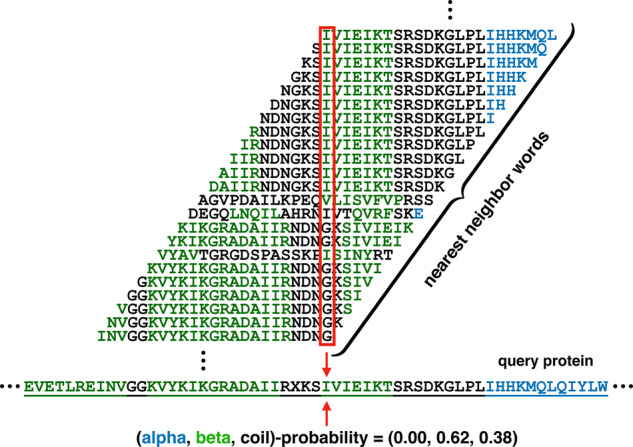
Template database words overlapping a given query residue contribute to its class membership probability. Across the bottom is a portion of the amino acid sequence of an actual query protein. Stacked above the residue highlighted by the arrows in the query sequence are the 1-nearest-neighbor words from our template database found for the query words containing the highlighted residue. The known secondary structure class of each amino acid is indicated by its color: blue for α, green for β and black for γ. The example is for word length 23, and positional weights ω from our implementation (namely, uniform across a word, except the central weight is doubled). For this word length and positional weights, the α-, β- and γ-class membership probabilities for the highlighted residue are 0.00, 0.62 and 0.38, respectively.

To handle the degenerate case of a boundary position i near the start or end of a protein without an amino acid word of length $\ell$ centered at i, we create a full border word padded out to length $\ell$ by putting dummy amino acid Z at the missing positions. We create border words at boundary positions when inserting template words into our database and extracting query words during prediction. We ensure query words have as nearest neighbors only template words with the same or fewer dummy symbols by making $\delta (a,b)\ll \delta (\mathtt{Z},\mathtt{Z})<\delta (a,\mathtt{Z})$ for $a,b\ne \mathtt{Z}$. Estimating structure probabilities at boundary positions then proceeds as described earlier.

2.2 Computing maximum likelihood protein structures

Given the residue class-membership probabilities for the protein, a straightforward greedy algorithm for prediction would simply output the highest-probability structure-class, independently at each residue. A failing of this natural greedy approach is that it does not necessarily output a physically valid secondary-structure prediction: runs of consecutive residues that share the same structure class are known to physically have minimum lengths, and a greedy prediction may violate these minimum run lengths. In contrast, we develop an efficient dynamic programming algorithm that is guaranteed to output a physically valid prediction that satisfies minimum run length constraints, while optimizing the structure class probabilities at residues, as well as other features of the prediction such as the rates of transitions between runs and the lengths of runs.

2.2.1 Maximum likelihood objective

Given a protein whose secondary structure we want to predict, that has amino acid sequence P of length n, we view a secondary structure prediction for the protein as a string S of length n over the secondary structure alphabet Σ. We index the positions of structure prediction S starting from 1.

Let $\mathcal{S}$ be the set of all valid secondary structure predictions for P: namely, the set of all strings of length n over alphabet Σ whose runs of a given structure class satisfy the minimum run-length requirements for physically valid secondary structures.

Our likelihood function on a prediction $S\in \mathcal{S}$ is a product of the probabilities that a secondary structure for P has the observed: (i) states of structure classes at the positions in S, (ii) transitions between classes at adjacent positions in S, and (iii) runs of the given lengths in S.

The contribution of the structure states in S to the likelihood is the product over positions i for $1\le i\le n$ of the class membership probability $\mathrm{Pr}(S[i] \text{occurs} \text{at} i)$.

The contribution of transitions in S to the likelihood is the product over positions i < n of the probability $\mathrm{Pr}(S[i] \text{followed} \text{by} S[i+1])$.

For the contribution of runs in S to the likelihood, for a position i let $\rho (i)$ be the length of the run of class $S[i]$ that extends to the left from position i. We assume that prediction S is terminated with a dummy symbol at $S[n+1]$ that is not in alphabet Σ (to capture the last run in S in the following product). The contribution of runs to the likelihood is then the product, over positions $1\le i\le n$ for which $S[i]\ne S[i+1]$, of the run-length probability $\mathrm{Pr}(\text{run} \text{of} S[i] \text{of} \text{length} \rho (i))$.

We denote the minimum run length for runs of structure class c by λ_c. In practice, when empirically measuring the probability of a run of length $\ell$, we explicitly record this empirical probability for runs of length $\ell <h$, for a fixed length upper bound h. (We ensure this length upper bound satisfies $h\ge {\max }_c{ \lambda }_c$.) The empirical probability that we then store for length h is really a lumped sum over all runs of length $\ell \ge h$.

We express our optimization problem as finding a prediction that minimizes the negative logarithm of the likelihood function. For residue position i, structure classes a, b, c and run length $\ell <h$, define

$$\begin{array}{c}p(i,c) :=-\text{log} \mathrm{Pr}(c \text{occurs} \text{at} i),\\ q(a,b) :=-\text{log} \mathrm{Pr}(a \text{followed} \text{by} b),\\ r(\ell ,c) :=-\text{log} \mathrm{Pr}(\text{run} \text{of} c \text{of} \text{length} \ell ),\\ r(h,c) :=-\text{log} \mathrm{Pr}(\text{run} \text{of} c \text{of} \text{length} \text{at} \text{least} h).\end{array}$$

We weight the relative contribution to the log-likelihood of terms due to probabilities for class membership p(i, c), transitions q(a, b) and lengths of runs $r(\ell ,c)$, by the respective coefficients $a_{\text{state}},\hspace{0.17em}{a}_{\text{trans}}$ and $a_{\text{run}}$.

The negative log-likelihood function that we optimize over structure predictions S is then,

$$\begin{array}{c}\mathcal{L}\left(S\right) := a_{\text{state}} \sum _{1\le i\le n} p(i,S[i\left]\right)\\ + a_{\text{trans}} \sum _{1\le i<n} q\left(S\right[i],S[i+1\left]\right)\\ + a_{\text{run}}\sum _{\begin{array}{c}1\le i\le n\\ S\left[i\right]\ne S[i+1]\end{array}}r(\rho (i),S[i\left]\right).\end{array}$$

Next we explain how to efficiently find a prediction $S\in \mathcal{S}$ that minimizes $\mathcal{L}(S)$, or equivalently, has maximum likelihood.

2.2.2 Dynamic programming algorithm

We find an optimal physically-valid prediction of maximum likelihood using dynamic programming, as follows.

Let $L(i,\ell ,c)$, for $\ell <h$, be the negative log-likelihood of an optimal prediction ending at position i, where position i is predicted to have structure class c and the run of class c ending at position i has length $\ell$. For $\ell =h$, quantity $L(i,h,c)$ is defined to be the negative log-likelihood of an optimal prediction ending in a run of length at least h.

The negative log-likelihood of an optimal prediction $S\in \mathcal{S}$ for a protein of length n is then ${\min }_{c\in \Sigma } {\min }_{{\lambda }_c\le \ell \le h} L(n,\ell ,c)$.

We now give recurrences for $L(i,\ell ,c)$ in general.

For structure class c and lengths $\ell$ in the range ${\lambda }_c<\ell <h$,

$$\begin{array}{c}L(i,\ell ,c) = a_{\text{state}} \hspace{0.17em}p(c,i)+a_{\text{trans}} \hspace{0.17em}q(c,c)\\ + \hspace{0.17em}{a}_{\text{run}}\left(r\right(\ell ,c)-r(\ell -1,c\left)\right)\hspace{0.17em}+\hspace{0.17em}L(i-1,\ell -1,c).\end{array}$$

For structure class c and length $\ell ={\lambda }_c$,

$$\begin{array}{c}L(i,{\lambda }_c,c)\hspace{0.17em}=\hspace{0.17em}{a}_{\text{state}}\sum _{i-{\lambda }_c < j \le i}p(j,c)\hspace{0.17em}+\hspace{0.17em}{a}_{\text{trans}}({\lambda }_c-1) q(c,c)\\ +\underset{b \ne c}{\min }\left\{\underset{{\lambda }_b \le k \le h}{\min }\{L(i-{\lambda }_c,k,b)\}+a_{\text{trans}}\hspace{0.17em}q(b,c)\right\}\\ +\hspace{0.17em}{a}_{\text{run}}\hspace{0.17em}r({\lambda }_c,c).\end{array}$$

For structure class c and length $\ell =h$,

$$\begin{array}{c}L(i,h,c) \hspace{0.17em}=\hspace{0.17em} a_{\text{state}}\sum _{i-h+{\lambda }_c < j \le i}^{}p(j,c)\\ + a_{\text{trans}} (h-{\lambda }_c) \hspace{0.17em}q(c,c)\\ + \underset{{\lambda }_c \le k \le h}{\min }\left\{\begin{array}{c}L(i-h + {\lambda }_c,k,c) +\\ \hspace{1em}{a}_{\text{run}} \left(r\right(h,c)-r(k,c\left)\right)\end{array}\right\}.\end{array}$$

Together the above recurrences specify how to compute $L(i,\ell ,c)$ for all ${\lambda }_c\le \ell \le h$ and ${\lambda }_c\le i\le n$. For the boundary values where $1\le i<{\lambda }_c$, we set $L(i,\ell ,c):=\infty$.

The dynamic programming algorithm uses the above recurrences to first fill in a three-dimensional table for $L(i,\ell ,c)$, in order of increasing i and $\ell$. It then finds the optimal entry, $\arg {\min }_{\ell ,c}\hspace{0.17em}L(n,\ell ,c)$, that corresponds to a complete prediction of minimum negative log-likelihood, and recovers an optimal prediction by tracing backward from this final entry. Since the length parameter $\ell$ satisfies ${\lambda }_c\le \ell \le h$ for constants λ_c and h, there are O(1) values for $\ell$; there are also O(1) values for c. So the table has $\Theta (n)$ entries, and filling in an entry by the recurrences takes O(1) time. Thus filling the entire table takes $\Theta (n)$ total time, which is also the time to recover the optimal prediction.

In short, the dynamic programming algorithm finds a physically-valid secondary structure prediction of maximum likelihood in $\Theta (n)$ time.

2.3 Estimating the accuracy of a structure prediction

A unique aspect of our core nearest-neighbor-based approach to secondary structure prediction is that, in addition to outputting a predicted structure, we can also provide an estimated accuracy for this prediction. While in practice it is normally not possible to measure the true Q₃ or Q₈ accuracy of a prediction (since the correct secondary structure for the protein is usually not known), we can actually estimate this unknown Q₃ or Q₈ accuracy reasonably well, based on the similarity of the overlapping nearest neighbor words (which vote on structure probabilities) to their corresponding query words.

Intuitively, as these nearest neighbor words that overlap at a given residue are closer to their query words for this residue, our confidence in the resulting structure probabilities at this residue should increase. More precisely, at each residue in a collection of proteins whose correct secondary structure is known, we measure the distances of the overlapping nearest neighbor words to their query words for this residue, and average these word distances for that residue. For residues in the protein collection, we know the correct secondary structure class for the residue, and we have the greedily predicted structure class of highest estimated probability. We then sort all residues in the protein collection by their average word distance, and for each residue in this sorted list, we measure the empirical accuracy of the residues within a window of the sorted list centered at that residue (namely a window consisting of the m consecutive residues with closest average distance below the residue, and the m consecutive residues with closest average distance above the residue), by counting how many residues in this window have a correctly predicted structure class, divided by the total number of residues in the window. Section 4.2 later shows that, as we would intuitively expect, the empirical residue accuracy measured in this way is in fact negatively correlated with the average word distance of residues. We then fit an estimator to this data from the protein collection on empirical accuracy versus word distance.

To obtain an accuracy estimate for an entire protein structure predicted by our core approach, we measure these average word distances at the residues of the protein, look up the corresponding empirical accuracy for these word distances using the fitted estimator, and then average these empirical accuracies across the residues in the protein. The resulting estimated accuracy of the structure prediction is reasonably close to the true accuracy of the prediction (in practice within roughly 5% and 8% on average for Q₃ and Q₈ accuracies, respectively) as discussed in Section 4.2.

This accuracy estimator is similar to the feature-based approach to accuracy estimation developed for parameter advising by DeBlasio and Kececioglu (2017), where the feature at residues is average word distance.

2.4 Constructing a hybrid predictor

When predicting on a protein whose amino acid words match well to our template database, this core template-based approach tends to achieve high accuracy, but for proteins without good template matches its accuracy can drop substantially. Fortunately, we can leverage our accuracy estimator to recognize when our core approach’s prediction is likely inaccurate, and in that situation invoke a non-template-based method. This leads to a natural hybrid approach, that combines the distinct advantages of both template-based methods (which are very accurate for proteins sufficiently similar to their template database) and non-template-based methods (which tend to be more stable and generalize better, though they usually do not reach the peak accuracies of template-based methods).

For structure prediction S, let $Q(S)$ be the estimated accuracy of this prediction using our estimator from Section 2.3. (Note that in reality our accuracy estimator uses information beyond simply the prediction S: namely, average word distances at residues.) The hybrid approach uses an accuracy threshold τ, as well as an alternate prediction method (ideally, complementary to our core approach) that supplies alternate prediction $S\prime$.

Our hybrid approach then simply evaluates accuracy estimator $Q$ on prediction S from our core approach, and if $Q(S)\ge \tau$, outputs S; otherwise, it invokes the alternate prediction method to output $S\prime$.

Surprisingly, this new hybrid approach significantly exceeds the average accuracy of both methods it hybridizes, as shown in Section 3.2.

3 Results

We present results from computational experiments with our core and hybrid approaches on evaluation datasets, and compare to state-of-the-art methods.

3.1 Datasets, evaluation, and implementation

Our template databases are drawn from proteins in the protein databank (PDB) (Berman et al., 2000). These proteins are split into words of length 23, for our nearest neighbor search. For method development and parameter tuning, our testing set consists of proteins deposited into PDB between October 1, 2018 and January 1, 2019, while the template database contains proteins deposited before October 1, 2018. For comparison to state-of-the-art methods, we use benchmark CASP datasets. All 129 proteins of the CASP10 dataset, all 105 proteins of the CASP11 dataset, all 55 proteins of the CASP12 dataset, and all 49 of the CASP13 dataset were used in our evaluation. The yearly datasets contain a random subset of proteins deposited into PDB each year from 2014 to 2019 (called PDB2014, … , PDB2019), except PDB2019, which contains all proteins deposited between January 1, 2019 and May 15, 2019. All dataset proteins have known secondary structure, and we remove any proteins shorter than 23 residues or with more than five ambiguous amino acids. For a fair evaluation, we also remove identical copies of proteins in the yearly datasets from our template database. We do not remove proteins from our template database that are similar to those in evaluation datasets, following the convention established by other template-based approaches (Pollastri et al., 2002). However, for every CASP dataset, our template database contains only proteins available 1 month before that CASP competition ended, simulating a template database available for the CASP competition.

3.1.1 Evaluation

We compare the accuracy of Nnessy, and the best hybrid of Nnessy with another tool, to state-of-the-art methods on the PDB2019 and CASP datasets, which we call the evaluation datasets. Other tools may have trained on proteins similar to the evaluation data, but we give them the benefit of the doubt, as these tools do not have an option to retrain with a new training set. Our evaluation on PDB2019 follows the convention of other template-based methods (Pollastri et al., 2002).

We also evaluate the accuracy of Nnessy on the six yearly datasets, consisting of proteins added to PDB each year for the past 6 years. For these datasets, we compare Nnessy, the best tool for 8-state and 3-state prediction, and the hybrid between them.

We use Q₃ and Q₈ accuracy to measure performance, which is the number of residues predicted correctly divided by the total number of residues in the protein. When we refer to the Q₃ or Q₈ accuracy of a dataset, we refer to the average accuracy of the proteins in that dataset.

3.1.2 Implementation and parameter tuning

We implemented our method in C/C++ and Python. We used cross-validation to tune the following parameters: word length ($\ell$), the number of neighbors found in nearest neighbor searches (k), positional weights for secondary structure words (ω) and weights on the terms in the maximum likelihood objective function.

Word length for the template database was chosen to be $\ell =23$, which maximizes the number of words in the template database. We found a strong correlation between larger template databases and higher-accuracy predictions. Word lengths in the range [13,33] were tested and accuracies differed by about 1%. The template database for the PDB2019 dataset (the largest template database) contains 24,312,377 length-23 words.

In the overlapping secondary structure words method discussed in Section 2.1, k is the number of neighbors returned from the template database for a given query word. We tuned the value of k to yield the highest accuracy on our testing set, and chose k = 3.

Positional weights ω for a secondary structure word used in the overlapping words procedure are uniform, except at the central position, where the weight is doubled.

In the negative log-likelihood objective function used in the dynamic programming algorithm, the coefficients put lower weight on transition rate (0.1) and run-length (0.1) terms, whereas coefficients for the other terms are 1. Run lengths were found over the template database, and the objective function weights were chosen using grid search over possible values.

3.2 Prediction accuracy

Table 1 compares the Q₈ accuracy of Nnessy, the hybrid method and state-of-the-art tools. The Q₈ accuracies in the table give the mean and standard deviation over the dataset. The hybrid boost for a tool shows the improvement in accuracy when hybridizing the tool with Nnessy. For all tools and datasets, the hybrid offers a boost in accuracy over either tool. The best Nnessy hybrid is the highest-accuracy hybrid between Nnessy and another tool. We evaluated the accuracies for other tools ourselves by either downloading the tool (PSIPRED, SSpro), or using a server for the tool (JPRED, PORTER, DeepCNF and PSRSM). For many of the tools, the accuracy shown in Tables 1 and 2 is higher than the accuracy reported in their paper, possibly due to the presence of evaluation proteins in their training sets. The hybrid method still achieves a boost in accuracy even over these higher accuracies.

Table 1.

Eight-state accuracies on CASP and PDB2019 datasets

	CASP10		CASP11		CASP12		CASP13		PDB2019
Number of proteins	129		105		55		49		292
Average protein length	177		183		188		280		281
		Hybrid		Hybrid		Hybrid		Hybrid		Hybrid
Tool	Q 8 accuracy	Boosta	Q 8 accuracy	Boosta	Q 8 accuracy	Boosta	Q 8 accuracy	Boosta	Q 8 accuracy	Boosta
Nnessy	67.4% ± 22.4		67.2% ± 21.3		55.5% ± 21.8		66.5% ± 21.1		82.4% ± 18.9
DeepCNF	69.6% ± 12.7	+6.1%	72.5% ± 8.0	+6.8%	68.2% ± 13.4	+2.8%	64.0% ± 11.4	+9.7%	68.7% ± 11.8	+14.1%
SSpro	77.3% ± 16.1	+3.9%b	77.9% ± 14.9	+4.8%b	62.5% ± 14.8	+3.5%	59.9% ± 16.6	+12.8%	73.9% ± 18.8	+7.7%
PORTER	75.6% ± 9.9	+5.2%	75.1% ± 8.2	+6.0%	70.9% ± 12.6	+2.4%b	65.2% ± 15.2	+10.4%b	70.5% ± 11.3	+12.6%b
Best Nnessy hybrid	81.2% ± 16.2		82.7% ± 14.4		73.3% ± 14.3		75.6% ± 14.4		83.1% ± 15.0

Highlighted table entries are in bold.

^aHybrid boost is the improvement in accuracy when hybridizing a tool with Nnessy.

^bThe tool that gave the best Nnessy hybrid for that dataset.

Table 2.

Three-state accuracies on CASP and PDB2019 datasets

	CASP10		CASP11		CASP12		CASP13		PDB2019
Number of proteins	129		105		55		49		292
Average protein length	177		183		188		280		281
		Hybrid		Hybrid		Hybrid		Hybrid		Hybrid
Tool	Q 3 accuracy	Boosta	Q 3 accuracy	Boosta	Q 3 accuracy	Boosta	Q 3 accuracy	Boosta	Q 3 accuracy	Boosta
Nnessy	75.5% ± 18.5		74.5% ± 17.0		67.9% ± 15.8		75.7% ± 16.3		85.7% ± 15.2
JPRED	78.3% ± 7.9	+5.6%	78.0% ± 7.0	+5.7%	75.9% ± 9.7	+2.8%	76.0% ± 9.1	+5.9%	77.6% ± 7.5	+9.4%
DeepCNF	81.8% ± 9.6	+4.1%	82.3% ± 6.0	+4.3%	79.8% ± 9.9	+1.9%	77.8% ± 8.6	+5.2%	81.3% ± 9.1	+6.0%
PSIPRED	84.8% ± 7.5	+3.5%	83.6% ± 5.8	+3.9%	80.0% ± 10.0	+2.1%	79.8% ± 8.1	+4.6%	79.7% ± 8.6	+7.5%
SSpro	85.4% ± 11.6	+2.5%	85.8% ± 10.5	+2.8%	75.2% ± 10.7	+2.8%	74.0% ± 11.4	+7.1%	82.6% ± 12.9	+4.2%
PORTER	85.3% ± 6.8	+3.1%	84.5% ± 6.2	+3.4%	81.8% ± 9.0	+1.8%	80.2% ± 10.0	+4.6%	83.1% ± 8.5	+4.6%
PSRSM	89.6% ± 9.3	+2.0%b	90.5% ± 7.7	+1.4%b	82.6% ± 12.2	+1.4%b	82.5% ± 12.7	+3.5%b	84.8% ± 10.2	+3.2%b
Best Nnessy hybrid	91.6% ± 9.2		91.8% ± 7.7		84.0% ± 12.0		85.9% ± 11.8		88.0% ± 9.2

Highlighted table entries are in bold.

^aHybrid boost is the improvement in accuracy when hybridizing a tool with Nnessy.

^bThe tool that gave the best Nnessy hybrid for that dataset.

Hybridization combines the strengths of template- and non-template-based tools. Template-based methods predict accurately when a close template match is found, while non-template-based tools predict well consistently and generalize to new data. With hybridization, we achieve a more robust, higher-accuracy tool than either single tool. Nnessy is the template-based tool in every hybrid, because the hybrid approach needs an accuracy estimator, which other template-based tools lack. The best hybrid method outperforms all other tools by more than 3% on every evaluation dataset, and by more than 10% on CASP13 and PDB2019. Hybridization also raises the accuracy of Nnessy substantially, around 15% on average for the CASP datasets.

Prediction accuracy variance is high for Nnessy because predictions for proteins with close template matches are very accurate, while poor template matches yield lower prediction accuracy. However, when Nnessy is hybridized with another tool, the hybrid accuracy variance is generally close to the variance of the other tool, due to the removal of many low-accuracy predictions. Surprisingly, hybridization raises the low accuracy of Nnessy above the accuracy of any other tool, which is discussed further in Section 4.3.

Table 2 compares the Q₃ accuracy of Nnessy, the hybrid method and state-of-the-art tools. For each tool, we give the accuracy boost from hybridizing it with Nnessy (as described in Section 2.4). The best Nnessy hybrid for 3-state prediction is always with PSRSM and the hybrid method boosts the Q₃ accuracy by 2.3% on average per evaluation dataset. Once again, despite the low accuracy of Nnessy on the CASP datasets, hybridizing any tool with Nnessy boosts the accuracy for that tool on all datasets. The accuracy variance follows the same trends as 8-state prediction, where the hybrid method reduces the variance of Nnessy to the level of the other hybridized tool.

Following other template-based methods (Pollastri et al., 2002), we evaluate our accuracy on proteins submitted to PDB each year, using proteins submitted previous to that year as a template database. Table 3 shows the accuracy of Nnessy, the best tools on CASP datasets for 3-state and 8-state prediction and the hybrid method between them evaluated on the yearly datasets. Unlike the CASP datasets, there is high sequence similarity between proteins in the yearly datasets and the template database. This yields high accuracies for Nnessy over other tools for 8-state prediction, with the hybrid method improving that accuracy even further. For 8-state prediction, template-based approaches offer higher prediction accuracies because there is more chance for confusion in non-template-based approaches. The variance in prediction accuracy follows the same trend as it did in Tables 1 and 2.

Table 3.

Eight- and three-state accuracies on yearly PDB datasets of the best tools

	PDB2014		PDB2015		PDB2016		PDB2017		PDB2018		PDB2019
8-State	Q 8 accuracy	Boosta	Q 8 accuracy	Boosta	Q 8 accuracy	Boosta	Q 8 accuracy	Boosta	Q 8 accuracy	Boosta	Q 8 accuracy	Boosta
PORTER	75.6% ± 7.4	+8.5%	74.9% ± 10.8	+8.8%	75.2% ± 11.2	+9.1%	73.6% ± 9.4	+10.1%	74.5% ± 9.6	+9.8%	70.5% ± 11.3	+12.6%
Nnessy	79.3% ± 18.1	+4.8%	80.6%± 16.4	+3.1%	82.5% ± 15.3	+1.8%	80.5% ± 17.4	+3.2%	82.8% ± 15.7	+1.5%	82.4% ± 15.2	+0.7%
Hybrid	84.1% ± 10.8		83.7% ± 12.3		84.3% ± 12.5		83.7% ± 12.7		84.3% ± 12.5		83.1% ± 15.0
3-State	Q 3 accuracy	Boosta	Q 3 accuracy	Boosta	Q 3 accuracy	Boosta	Q 3 accuracy	Boosta	Q 3 accuracy	Boosta	Q 3 accuracy	Boosta
Nnessy	85.5% ± 12.9	+2.3%	85.3% ± 22.0	+6.0%	87.3% ± 12.0	+2.9%	84.9% ± 12.8	+4.2%	85.7% ± 10.7	+2.3%	85.7% ± 15.2	+2.3%
PSRSM	87.6% ± 8.4	+0.2%	87.2% ± 8.4	+4.1%	88.5% ± 6.0	+1.7%	86.0% ± 13.3	+3.1%	88.0% ± 9.1	+0.0%	84.8% ± 10.2	+3.2%
Hybrid	87.8% ± 8.7		91.3% ± 7.6		90.2% ± 9.2		89.1% ± 11.9		88.0% ± 9.1		88.0% ± 9.2

Highlighted table entries are in bold.

^aBoost is the improvement in accuracy of the hybrid over the original tool.

The maximum-likelihood dynamic programming approach enables Nnessy to output physically valid secondary structure predictions, while raising the average accuracy by about 0.1% for all datasets.

4 Discussion

We discuss accuracy as a function of template database size, fidelity of accuracy estimation, behavior of the hybrid approach, and running time.

4.1 Accuracy versus template database size

With larger template databases, Nnessy tends to get higher accuracy. We measure the tradeoff between template database size and accuracy by randomly subsampling our template database and then predicting on PDB2019 using these smaller databases. Figure 2 shows the tradeoff of Q₃ and Q₈ accuracy versus template database size. Our accuracy remains stable until more than 50% of the words are removed from the template database. This may be due to redundancy among overlapping words, where removing random words from long runs of nearest neighbors with near-identical secondary structure has little effect on overall accuracy.

Fig. 2.

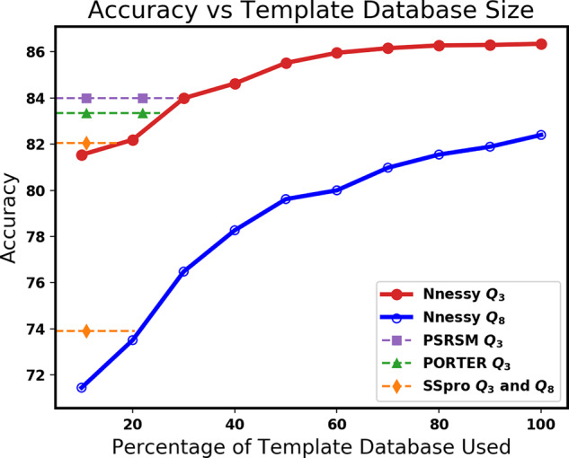
Average accuracy on PDB2019, using a fraction of the full template database. The horizontal axis is the percentage of the full template database used, for a random subset of the database. The vertical axis is the accuracy on PDB2019. The solid curves in the plot give the Q₃ and Q₈ accuracy of Nnessy. Dashed lines represent the accuracy of other methods on PDB2019; their intersection point with a curve gives the fractional size of the template database at which Nnessy meets their accuracy. Only tools whose accuracies intersect each curve are shown. By reducing its template database size, Nnessy can be further sped up, and still exceed the accuracy of state-of-the-art tools on such datasets.

Figure 2 also shows the accuracy achieved by methods whose Q₃ or Q₈ accuracies intersect the respective curve. Our current implementation of the core method has running time proportional to the size of the template database, so reduced template database size roughly correlates with reduced running time. Nnessy could use a template database of 30% size and still match the accuracy of the next-best method on PDB2019, while running about three times faster than our current implementation. It is possible that a careful subsampling (where we remove words systematically instead of randomly) could achieve even better results.

4.2 Performance of the accuracy estimator

Nnessy uses the distance to the overlapping nearest neighbors of each residue to estimate prediction accuracy. Figure 3 shows the average accuracy of residues, given the average nearest neighbor distance of their overlapping words. Each blue circle represents a residue from the evaluation datasets, with the average distance of its overlapping nearest-neighbor words given on the horizontal axis, and the empirical average accuracy of the 100 residues with closest average word distance given on the vertical axis. We fit lines to the two portions of the plot, which are used for accuracy estimation. Residue accuracy does not change much with increasing distance until around a distance of 0.6, where the accuracy begins to plummet with increased distance. To estimate prediction accuracy of a protein, we average the estimated residue accuracy across the protein.

Fig. 3.

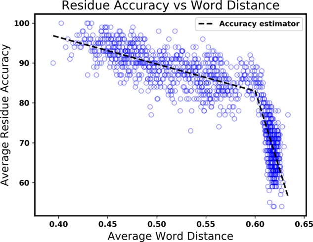
Comparison of residue accuracy to overlapping word distance. Each blue circle represents a residue from the evaluation datasets, with the average distance of its overlapping nearest-neighbor words given by the horizontal axis, and the average accuracy of the 100 residues with closest average word distance shown on the vertical axis. The dashed lines show the fitted accuracy estimator, which gives the estimated probability that the predicted state of a residue is correct, as a function of its average word distance.

Figure 4 shows the true Q₃ accuracy compared to the estimated accuracy for each protein in the evaluation datasets. The green and red discs give the average accuracy compared to the average estimated accuracy for an evaluation or yearly dataset. The black dashed line shows the identity, where predicted accuracy equals true accuracy. On average, the accuracy estimator has error of 5.3% for 3-state predictions and 8.3% error for 8-state predictions on the evaluation datasets. For 8-state prediction, the plots look roughly the same for both Figures 3 and 4. For each of the evaluation datasets, the estimated accuracy of a protein is from an estimator fitted on evaluation datasets that do not include the protein.

Fig. 4.

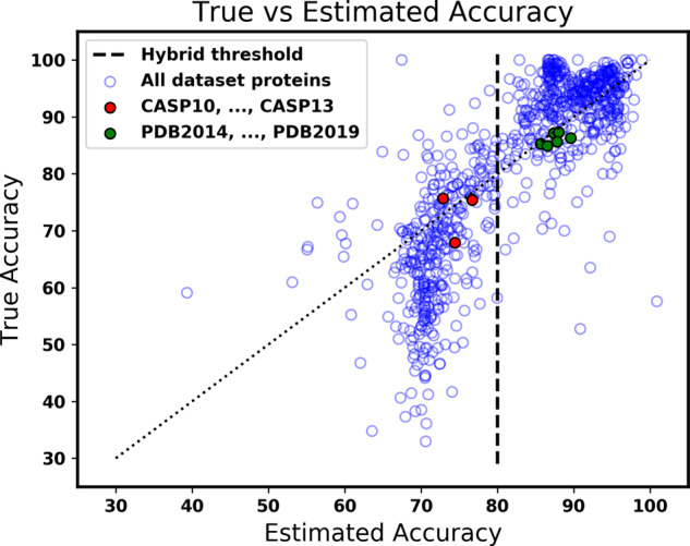
Comparison of true and estimated accuracy for our accuracy estimator. The blue circles represent proteins from all datasets, with the estimated accuracy of the Nnessy prediction for the protein shown on the horizontal axis, and the true accuracy of the prediction on the vertical axis. Along the dotted line, estimated accuracy is equal to true accuracy. The dashed line is at the threshold used by our hybrid method; circles to its right are Nnessy predictions chosen by the hybrid method. The red discs show the average true accuracy and average estimated accuracy of proteins in the four CASP datasets; green discs show the same for the six PDB datasets. The estimated accuracy of a protein is from an estimator fitted on evaluation datasets that do not include that protein. The closer a circle is to the dotted line, the more accurate the accuracy estimator.

4.3 Performance of the hybrid approach

The hybrid approach combines the best predictions from Nnessy with the robust predictions from a non-template-based tool. We estimate the prediction accuracy for a protein based on the distance of overlapping nearest neighbor words for each residue as detailed in Section 4.2. If the estimated accuracy is above a threshold (80%), Nnessy’s prediction is output as the hybrid prediction. Otherwise the prediction of the other hybridized tool is chosen. We chose 80% as the threshold because, for Nnessy, few proteins have estimated accuracy greater than 80%, but true accuracy lower than 80% (see Fig. 4). Therefore, the hybrid approach rarely chooses a low-accuracy prediction from Nnessy. When no close template matches are found (the nearest-neighbor distance is high), non-template-based tools generally have higher accuracy than Nnessy, due to better generalization, so their prediction is used.

The hybrid approach chooses predictions near-optimally, where the optimal choice is the prediction with higher true accuracy. The following table compares the accuracies of: Nnessy, the next-best tool on the CASP datasets (PORTER for 8-state and PSRSM for 3-state), the hybrid of the two tools with randomly chosen predictions, the hybrid with an 80% threshold, and an oracle that picks the highest-true-accuracy prediction. All accuracies are averaged over the CASP datasets.

	Nnessy	PORTER	PSRSM	Random	Hybrid	(Oracle)
8-State	64.2%	71.7%		68.0%	77.7%	(78.1%)
3-State	73.4%		86.3%	79.8%	88.3%	(88.9%)

The hybrid method is usually within 1% of the oracle and is even optimal in some cases (for the hybrid of Nnessy and PORTER on CASP10). This demonstrates that the hybrid method selects predictions much better than random, and the simple, thresholded hybrid method approaches optimal prediction selection. The per-residue hybrid approach, where the hybrid chooses which prediction to output at the residue level instead of the protein level, has a higher oracle accuracy, but in practice a simple 80% threshold for the per-residue hybrid approach did not outperform the per-protein hybrid.

In Figure 5, we visualize the selections made by the hybrid approach. We sorted the proteins in the CASP dataset by the Q₈ accuracy of the PORTER-Nnessy hybrid, and the protein rank of this sorting is given on the horizontal axis. A blue circle and green triangle are plotted for each protein giving the Q₈ accuracy of PORTER and Nnessy on the vertical axis, respectively. The black curve goes through the prediction the hybrid selected for each protein. Points above and below the line respectively indicate suboptimal and optimal choices made by the hybrid approach, where choosing the higher-accuracy prediction is optimal. Due to the high variance in the prediction accuracy of Nnessy, as shown by the accuracy spread of circle markers in the plot, on CASP datasets the hybrid approach chooses 19% of Nnessy’s 8-state predictions, and 25% of its 3-state predictions. On the other hand for the PDB datasets, the hybrid chooses 70% of Nnessy’s 8-state predictions and 83% of its 3-state predictions.

Fig. 5.

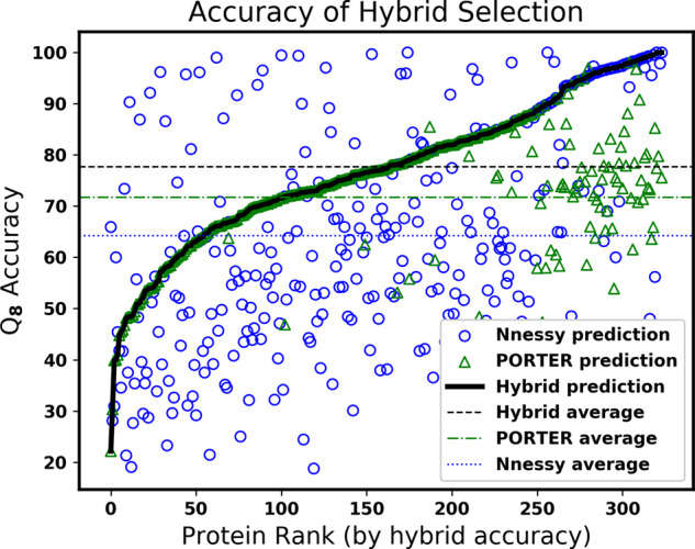
Visualization of the hybrid method. Each value along the horizontal axis corresponds to a single protein from CASP datasets. These CASP proteins are sorted along this axis by their Q₈ accuracy for the Nnessy-PORTER hybrid. At the rank of each such protein in this sorted order, a blue circle and a green triangle are plotted, with the vertical axis giving the Q₈ accuracy of their Nnessy and PORTER prediction, respectively. The solid black curve goes through the prediction that is selected by the hybrid method. Circles or triangles above this curve correspond to proteins for which the hybrid selection has suboptimal accuracy, while all those below are proteins for which the hybrid method is optimal.

4.4 Running time

The core method of Nnessy circumvents a traditional homology search, offering a speedup over a PSI-BLAST search of large protein sequence databases. We ran the following experiment using four cores of a Xeon Broadwell E5-2695 Dual 14-core, 2.3 GHz processor with 24 GB of memory. We measured the processing time for proteins in the CASP datasets, and Nnessy takes 1.4 s per residue, or on average 5 min to process a 200-length protein. PSI-BLAST over Uniref50 (used by SSpro) takes 2.7 s per residue, or on average 9 min to process a 200-length protein. PSI-BLAST over Uniref90 (used by PSIPRED) takes 9.6 s per residue, or 32 min on a 200-length protein. Our current implementation is nearly twice as fast as SSpro, and over six times faster than PSIPRED. The nearest neighbor searches of Nnessy are readily parallelized by distributing queries to separate jobs.

5 Conclusion

Our core approach to protein secondary structure prediction replaces the sequence database homology searches of current methods with a faster nearest neighbor search over a smaller template database of fixed-length words. Our hybrid approach, which combines this core method with an alternate non-template-based method, is the most accurate approach currently available for both 3- and 8-state secondary structure prediction.

References

- Adamczak R. et al. (2004) Accurate prediction of solvent accessibility using neural networks-based regression. Proteins, 56, 753–767. [DOI] [PubMed] [Google Scholar]
- Altschul S.F. et al. (1997) Gapped BLAST and PSI-BLAST: a new generation of protein database search programs. Nucleic Acids Res., 25, 3389–3402. [DOI] [PMC free article] [PubMed] [Google Scholar]
- Berman H. et al. (2000) The Protein Data Bank. Nucleic Acids Res., 28, 235–242. [DOI] [PMC free article] [PubMed] [Google Scholar]
- Beygelzimer A. et al. (2006) Cover trees for nearest neighbor. In Proceedings of the 23rd International Conference on Machine Learning (ICML). [CrossRef][10.1145/1143844.1143857]
- DeBlasio D., Kececioglu J. (2017) Parameter Advising for Multiple Sequence Alignment, Volume 26 of Computational Biology Series. Springer International. Cham, Switzerland. [Google Scholar]
- Deng X., Cheng J. (2011) MSACompro: protein multiple sequence alignment using predicted secondary structure, solvent accessibility, and residue–residue contacts. BMC Bioinformatics, 12, 472. [DOI] [PMC free article] [PubMed] [Google Scholar]
- Dill K.A., MacCallum J.L. (2012) The protein-folding problem, 50 years on. Science, 338, 1042–1046. [DOI] [PubMed] [Google Scholar]
- Dor O., Zhou Y. (2006) Achieving 80% ten-fold cross-validated accuracy for secondary structure prediction by large-scale training. Proteins Struct. Funct. Bioinf., 66, 838–845. [DOI] [PubMed] [Google Scholar]
- Drozdetskiy A. et al. (2015) JPred4: a protein secondary structure prediction server. Nucleic Acids Res., 43, W389–W394. [DOI] [PMC free article] [PubMed] [Google Scholar]
- Faraggi E. et al. (2012) SPINE X: improving protein secondary structure prediction by multistep learning coupled with prediction of solvent accessible surface area and backbone torsion angles. J. Comput. Chem., 33, 259–267. [DOI] [PMC free article] [PubMed] [Google Scholar]
- Finn R.D. et al. (2011) HMMER web server: interactive sequence similarity searching. Nucleic Acids Res., 39, W29–W37. [DOI] [PMC free article] [PubMed] [Google Scholar]
- Heffernan R. et al. (2015) Improving prediction of secondary structure, local backbone angles, and solvent accessible surface area of proteins by iterative deep learning. Sci. Rep., 5, 11476. [DOI] [PMC free article] [PubMed] [Google Scholar]
- Jones D. (1999) Protein secondary structure prediction based on position-specific scoring matrices. J. Mol. Biol., 292, 195–202. [DOI] [PubMed] [Google Scholar]
- Kabsch W., Sander C. (1983) Dictionary of protein secondary structure: pattern recognition of hydrogen-bonded and geometrical features. Biopolymers, 22, 2577–2637. [DOI] [PubMed] [Google Scholar]
- Kececioglu J. et al. (2010) Aligning protein sequences with predicted secondary structure. J. Comput. Biol., 17, 561–580. [DOI] [PubMed] [Google Scholar]
- Li D. et al. (2012) A novel structural position-specific scoring matrix for the prediction of protein secondary structures. Bioinformatics, 28, 32–39. [DOI] [PubMed] [Google Scholar]
- Lu Y., Sze S.H. (2008) Multiple sequence alignment based on profile alignment of intermediate sequences. J. Comput. Biol., 15, 767–777. [DOI] [PubMed] [Google Scholar]
- Ma Y. et al. (2018) Protein secondary structure prediction based on data partition and semi-random subspace method. Sci. Rep., 8, 9856. [DOI] [PMC free article] [PubMed] [Google Scholar]
- Mirabello C., Pollastri G. (2013) Porter, PaleAle 4.0: high-accuracy prediction of protein secondary structure and relative solvent accessibility. Bioinformatics, 29, 2056–2058. [DOI] [PubMed] [Google Scholar]
- Müller T. et al. (2002) Estimating amino acid substitution models: a comparison of Dayhoff’s estimator, the resolvent approach and a maximum likelihood method. Mol. Biol. Evol., 19, 8–13. [DOI] [PubMed] [Google Scholar]
- Pollastri G. et al. (2002) Improving the prediction of protein secondary structure in three and eight classes using recurrent neural networks and profiles. Proteins Struct. Funct. Bioinf., 47, 228–235. [DOI] [PubMed] [Google Scholar]
- Qi Y. et al. (2012) A unified multitask architecture for predicting local protein properties. PLoS One, 7, e32235. [DOI] [PMC free article] [PubMed] [Google Scholar]
- Saraswathi S. et al. (2012) Fast learning optimized prediction methodology (FLOPRED) for protein secondary structure prediction. J. Mol. Model., 18, 4275–4289. [DOI] [PMC free article] [PubMed] [Google Scholar]
- Spencer M. et al. (2015) A deep learning network approach to ab initio protein secondary structure prediction. IEEE/ACM Trans. Comput. Biol. Bioinf., 12, 103–112. [DOI] [PMC free article] [PubMed] [Google Scholar]
- Wang S. et al. (2016) Protein secondary structure prediction using deep convolutional neural fields. Sci. Rep., 6, 18962. [DOI] [PMC free article] [PubMed] [Google Scholar]
- Woerner A. (2016) On the neutralome of great apes and nearest neighbor search in metric spaces. PhD dissertation, Graduate Interdisciplinary Program in Genetics, University of Arizona, Tucson, Arizona, USA.
- Yang Y. et al. (2016) Sixty-five years of the long march in protein secondary structure prediction: the final stretch? Brief. Bioinf., 19, 482-494. [DOI] [PMC free article] [PubMed] [Google Scholar]
- Yaseen A., Li Y. (2014) Context-based features enhance protein secondary structure prediction accuracy. J. Chem. Inf. Model., 54, 992–1002. [DOI] [PubMed] [Google Scholar]