Factorized embeddings learns rich and biologically meaningful embedding spaces using factorized tensor decomposition

Abstract

Motivation

The recent development of sequencing technologies revolutionized our understanding of the inner workings of the cell as well as the way disease is treated. A single RNA sequencing (RNA-Seq) experiment, however, measures tens of thousands of parameters simultaneously. While the results are information rich, data analysis provides a challenge. Dimensionality reduction methods help with this task by extracting patterns from the data by compressing it into compact vector representations.

Results

We present the factorized embeddings (FE) model, a self-supervised deep learning algorithm that learns simultaneously, by tensor factorization, gene and sample representation spaces. We ran the model on RNA-Seq data from two large-scale cohorts and observed that the sample representation captures information on single gene and global gene expression patterns. Moreover, we found that the gene representation space was organized such that tissue-specific genes, highly correlated genes as well as genes participating in the same GO terms were grouped. Finally, we compared the vector representation of samples learned by the FE model to other similar models on 49 regression tasks. We report that the representations trained with FE rank first or second in all of the tasks, surpassing, sometimes by a considerable margin, other representations.

Availability and implementation

A toy example in the form of a Jupyter Notebook as well as the code and trained embeddings for this project can be found at: https://github.com/TrofimovAssya/FactorizedEmbeddings.

Supplementary information

Supplementary data are available at Bioinformatics online.

1 Introduction

RNA sequencing (RNA-Seq) data offer a snapshot into all the cellular processes at a specific time. Since the development of high-throughput sequencing, a multitude of other types of -omics experiments have appeared. RNA-Seq remains nonetheless the most accessible functional characterization of a biological sample. It is sufficiently mature to be applied in a clinical context and large-scale datasets of several thousands samples are readily available. In practice, once aligned and quantified, each RNA-Seq experiment yields (for a human sample) a vector of 20K to 60K gene expression values, depending on the gene annotation selected. Most analyses involving transcriptomic data, however, apply some kind of filtering on the genes by either selecting some of them, grouping them by function, or most of the time applying some type of dimensionnality reduction (Gibbons and Roth, 2002; Gönen, 2009; Kim and Kim, 2018).

Dimensionality reduction algorithms popular in bioinformatics analyses are principal components analysis (PCA), t-stochastic neighbourhood embeddings (t-SNE) (Van Der Maaten et al., 2009) and uniform manifold approximation and projection (UMAP) (McInnes et al., 2018). They all compress and encode (embed) the data into a new vector representation. While this is often done on samples, it is seldom done on genes. We found that gene representations are mainly computed in the context of clustering and factorization of genes into meta-genes (Brunet et al., 2004; Lemieux et al., 2017), with the ultimate goal of looking for molecular patterns in the gene expression data.

Some teams argue for a similarity between gene expression and bag-of-word representations of text corpora (Asgari and Mofrad, 2015; Ng, 2017), linking their work to that of Mikolov et al. (2013) and Pennington et al. (2014), who introduced distributed vector representations of words to the field of natural language processing. Upon training their models on word co-occurrences in context, they found that their representation of words captured some semantic relationships. This result is consistent with the distributional hypothesis in linguistics, where words with similar meaning will be found in similar contexts (Harris, 1954).

Inspired by their seminal work, Du et al. have used gene co-expression data to train gene embeddings they called gene2vec, and reported that their embeddings extract information of both gene type (protein coding, lncRNA, etc.) as well as tissue specificity (Du et al., 2019). Recently, Schreiber et al. have published Avocado, a deep neural network tensor factorization tool specialized in epigenomics data, that learns a representation of the human genome, allowing for imputation of epigenomics data and other related tasks (Schreiber et al., 2019). Lastly, similar work by Choy et al. showcased a shallow artificial neural network (ANN) to represent genes and samples in high-dimensional embedding spaces, while simultaneously extracting information about genes and samples (Choy et al., 2019). Choy et al. reported that they were able to cluster cancers according to gene expression into meta-groups that may then be used for predicting immune checkpoint therapy responders (Choy et al., 2019).

In principle, the model proposed by Choy et al. (2019) yields an attractive for data-mining double representation of genes and samples. In this aticle, we extend the idea behind simultaneously training a distributed representation for genes and samples, presented in Choy et al. (2019) to the notion of factorized embeddings (FE), an ANN that learns independent embedding spaces to represent factors of RNA-Seq data. We present the general framework of the FE model and compare it, when possible, to the models from Choy et al. (2019) and Du et al. (2019), as well as other standard dimensionality reduction algorithms such as t-SNE, UMAP and PCA. We show that FE capture biologically meaningful information and are reusable in auxiliary tasks that involve predicting some biological features of the dataset.

2 Approach

We term FE the idea behind training a distributed representation for genes or samples by factorized tensor decomposition. In transcriptomics, to describe a single gene expression value, we refer to ‘gene Y in sample X’; we propose to treat both samples and genes as factors that contribute to characterizing the data. Learning a FE of the data would be learning an embedding space for each of the factors that contribute to the gene expression value variation.

2.1 The factorized embeddings model

Each gene expression measurement is a single positive real number. Each single measurement x_ij is minimally characterized by a sample i it came from and a gene j it is measuring. Both the sample and the gene are the minimal descriptors for this single gene expression measurement. There may also be other additional descriptors that may influence the gene expression measurement, such as patient, batch, sex, race, etc. The data are cast into a narrow format, where each single measurement x_ij for sample i and gene j is described by a series of descriptors.

For clarity, the dataset was built using the two minimal descriptors: The data X is an N × M array, where there are N samples each of M gene expression measurements.

$$X=[x_1,x_2,\dots ,x_N]$$

So, an RNA-Seq sample i is represented by a vector of M real values.

$$x_i=[x_{i,1},x_{i,2},\dots ,x_{i,M}]$$

For each sample i and for each gene j in X, an entry in the dataset is created. X is transformed into the following two vectors, where the first contains indices tuples and the second the measured gene expressions $x_{i,j}$:

$$\left[\begin{array}{c}(1,1)\\ (1,2)\\ ⋮\\ (i,j)\\ ⋮\\ (N,M)\end{array}\right]\left[\begin{array}{c}{x}_{1,1}\\ x_{1,2}\\ ⋮\\ x_{i,j}\\ ⋮\\ x_{N,M}\end{array}\right]$$

Here, each entry in the table on the right is a gene expression measurement for sample i for all genes 1 to M. The table on the left is the descriptor table, where the identity of the sample i as well as the corresponding gene j are recorded. The descriptor table is the input for the neural network, where each doublet of values is an example, while the table on the right contains the targets.

We built a neural network where each of the inputs is embedded in a low-dimensional space of size k. For each field in the inputs, a function f maps a descriptor into a k-dimensional space $f:\mathbb{N}\to {\mathbb{R}}^k$. These spaces are referred to in the text as embedding or representation spaces. All k-dimensional coordinates in embeddings space are concatenated and serve as input for a multi-layer perceptron (MLP). The embedding of an input pair of descriptors (i, j) (e.g. sample i and gene j) is done with two functions $f_{\mathit{sample}}:i\to z_{\mathit{sample}}$ and $f_{\mathit{genes}}:j\to z_{\mathit{gene}}$ resulting in the following concatenated input for the MLP: $[z_{\mathit{sample}},z_{\mathit{gene}}]$, where Z_sample and Z_gene are the k-dimensional embedding spaces in which are represented, respectively, the samples 1 through N and the genes 1 through M.

The concatenated embedding coordinates are then fed through a series of fully connected layers (collectively referred to as g) and the final output layer is a single linear neuron, predicting the gene expression ${\widehat{x}}_{ij}$ for the corresponding descriptors sample i and gene j.

$$g(z_{\mathit{sample}},z_{\mathit{gene}})={\widehat{x}}_{ij}$$

All parameters ($\{\theta ,{\theta }_s,{\theta }_g\}$) for each layer as well as the embedding functions ($\{f_{{\theta }_s},f_{{\theta }_g}\}$) are optimized together by gradient descent with a mean-squared error (MSE) loss:

$$L=\frac{1}{N}\sum _{i=1}^N\sum _{j=1}^M(g_{\theta }(f_{{\theta }_s}(i),f_{{\theta }_g}(j))-x_{ij}{)}^2$$

This model functions with the assumptions that both the samples and features are independent and identically distributed (IID) amongst themselves (Murphy, 2012). While this may technically not be the case, we found most gene expression analyses work under the assumption of IID genes and IID samples (Maciejewski, 2014). Moreover, the FE model, by design, attempts to preserve all associations in the data between samples and features. We found that this may be in some cases a limitation, especially when the underlying data structure is not linear in the feature space (Supplementary Fig. S3). We tested the limits of the FE model on a series of toy datasets (Supplementary Figs S3–S6) and have made these experiments available in the Supplementary Material section.

3 Materials and methods

3.1 RNA-Seq data

RNA-Seq data for Genotype-Tissue Expression (GTEx) and The Cancer Genome Atlas (TCGA) cohorts were downloaded from the Xena Browser (Goldman et al., 2020). Xena browser offers a platform of re-aligned and quantified data using the same pipeline to allow for comparison across datasets and across experiments. For each dataset, the RNA-Seq reads were pseudo-aligned and quantified with Kallisto (Bray et al., 2016). Gene expression is represented by transcript per million (TPM) counts. Values were log-transformed with ${\hspace{0.17em}\text{log}\hspace{0.17em}}_{10}(\text{TPM}+1)$.

3.2 Tissue-specificity measures

To group genes by tissue specificity, two methods were used. The first, the Tau index τ as described by Yanai et al. (2005), is a measurement of how tissue-specific a gene expression is, comparing to the other samples. Briefly, for each tissue type c in C, the average expression is calculated for all genes and divided by the maximal value. Then, for each gene j, the τ_j is calculated with:

$${\tau }_j=\frac{{\sum }_{c=1}^C(1-x_{j,c})}{C-1}$$

The Tau index yields a single value between 0 and 1 for each gene. Yanai et al. categorize Tau index values between 0 and 0.3 as housekeeping genes and values above 0.8 as tissue-specific genes (Yanai et al., 2005).

The second one, the tissue-type Earth-Mover’s distance (EMD) is the Wasserstein distance for each tissue type done as following. Given a gene expression matrix of N samples by M genes, and for a vector tissues C, where each sample i has a tissue $c\in C$. For each gene $j\in M$ and each tissue $c\in C$, we calculate the tissue-specific EMD as the Wasserstein distance between the gene expression of gene j for all samples that belong to class c and the ones of other classes:

$$d_{EM{D}_j,c}=d_{\mathit{EMD}}(X[1_{x\in c},j],X[1_{x\notin c},j])$$

Thus, for every tissue type, we obtain a measure of information content for each gene, to distinguish between this tissue type and the others.

3.3 Replicating the results of similar models

We attempted to replicate the results published by Choy et al. (2019) in order to use their model for comparison to the FE model. However, despite significant efforts, we were unable to reproduce embeddings of the quality they presented using the approach as it is described in their publication. We therefore could only compare our FE model on the basis of the published embedding weights available on the author’s Github. Consequently, for these comparisons, we trained our FE model on the data processed the same way as described in their publication. Through this work, we maintain comparisons to the Choy model when possible.

For the gene2vec model published by Du et al., since it only creates representations of genes, we compared in (Section 3.8.1) their reported gene representation to the one learned by the FE model.

3.4 Benchmarks

For each task, we trained a k-nearest neighbours (kNN) regressor model. Similar to the kNN classifier, the regressor model finds k neighbours for a new point and outputs the average value for those points (instead of the majority class). The kNN was trained on 80% of the data and tested on 20%; this was repeated 100 times for each task. The performance was measured as the Pearson correlation coefficient between the predicted and the actual value. The choice for the correlation was to promote proportional values instead of exact values.

3.5 Statistical tests

To compare performances for classifiers trained on various embeddings, we performed an ANOVA test followed by Tukey post hoc testing. Differences in performance were considered statistically significant when the corrected P-value was lower than 0.05.

3.6 Model training

The entire FE model, which includes both embedding spaces and subsequent fully connected layers (see Section 2.1), is trained with a MSE loss function and $\tanh$ activation function, Adam optimizer, a L2 regularisation of ${10}^{-5}$ and a learning-rate of ${10}^{-3}$. The model is implemented in PyTorch (Paszke et al., 2019) and we release the code online (https://github.com/TrofimovAssya/FactorizedEmbeddings). We chose an embedding size of 50-dimensional for both genes and samples and a MLP of 5 layers, respectively of sizes 250, 150, 100, 50 and 10 (see Supplementary Figs). As a reference, for a dataset of 1 000 samples each of 60k transcript expression measurements, the model trains 500 epochs in 72 h on an NVIDIA GTX 1080 Ti.

3.7 Reconstruction accuracy of the model

As a sanity check, we first compared pair-wise distances between 1500 random sample pairs in original and reconstructed space (Fig. 1B). This was done to probe if once the data passes through the model, it preserves the proportions between samples. We found that the FE model reconstructs with high accuracy the data (Fig. 1B).

Fig. 1.

The factorized embeddings (FE) model reconstructs data with high accuracy and preserves sample pair-wise distances. (A) Schema of the FE model. (B) Pair-wise Euclidean distance preservation between 1500 random pairs of samples in original feature space (gene expression) and reconstructed space. (C, D) The FE-trained representation preserves more accurately than t-SNE pair-wise distances between samples in the embedding space. (E) The FE model allows for precise imputation of transcriptomes on a patient-level

Moreover, unlike the locally linear embeddings (LLE) (Roweis and Saul, 2000) algorithm or to some extent t-SNE, the FE model is not guaranteed to preserve sample-sample distances in the embedding space. We however report that it is the case for FE, where pair-wise distances in original feature space for a random subset of pairs of samples are preserved in embedding space (Fig. 1C), incidentally better than t-SNE (Fig. 1D).

We finally probed whether the gene expression reconstruction was performing well on hard to predict genes. We randomly selected 20 individuals for every tissue type in the GTEx cohort and compared the reconstructed by the FE model transcriptome as follows (Fig. 1E):

• itself (tissue+/sex+/person+)

• other samples of that tissue type, with matching sex (tissue+/sex+/person-)

• other samples of that tissue type, with opposite sex (tissue+/sex+/person-)

• other tissues for that individual (tissue-/sex+/person+)

We found that the reconstruction of the transcriptomes was always closer to the individual than to other matching tissue samples (Fig. 1E), with a Pearson’s correlation R² close to 1. As expected, other tissues for that individual were always less similar to the patient than other examples of the same tissue. We also found that depending on the tissue type, the other samples of the same tissue were at varying degrees of similarity, some closer as seen for Spleen and Breast and some quite far, such as Blood and Small Intestine (Fig. 1E). We hypothesize that since each sample represents a bulk tissue, some tissues might have a higher heterogeneity, with multiple cell lineages represented in each cell subset (Regev et al., 2017; Wagner et al., 2016). We limit the comparison in reconstruction to genes with a tissue-specific Earth-Mover’s distance over the 65th percentile (see Section 3), in other words, genes with high tissue specificity. While the 65th percentile was selected arbitrarily, the importance to use percentiles is caused by the fact that the EMD distribution for genes varies between tissue types and so the cutoff value might vary from tissue to tissue. We do this because we expect the large proportion of non-tissue-specific genes (e.g. housekeeping genes) to be well reconstructed and we want to probe the reconstruction of challenging genes.

Taken together, these results suggest that the FE model reconstructs with good accuracy each individual sample and preserves the sample pair-wise distances in the embedding space.

3.8 Factorized embeddings captures biologically meaningful information on both samples and genes

We found that similarly to t-SNE, the FE model trained on the GTEx dataset groups samples by tissue types and the FE model trained on the TCGA dataset groups samples by cancer types. For t-SNE, grouping of samples in embedding space depends on sample pair-wise distances, since this is what t-SNE optimizes locally in the representation (Van Der Maaten et al., 2009). This characteristic is however not guaranteed in FE, although we found that it is conserved (Fig. 1C).

For the results presented in Figure 2, we chose four ‘reporter’ genes or groups of genes (displayed for each column) for the following characteristics: (i) MYL2, coding for myosin 2 was chosen since it is expressed only by a small number of tissues (heart and muscle), (ii) CD8B, a marker of T cells was chosen because it is expressed in small quantities by many tissues and in high proportion in blood and spleen, (iii) XIST, a sex-specific gene, expressed only in tissues belonging to female individuals and (iv) keratin, a group of proteins expressed widely in epithelial tissues. For each of these reporter genes, we wanted to observe how the level of their expression across samples was represented in the embedding space. We found that the FE model learns a space where the predicted gene expression for genes that are common (keratin) or rare (MYL2) across tissues, regardless of their level of expression (CD8B) is smooth (Fig. 2, lower row). In contrast, we do not find the same smoothness with the t-SNE representation of the sample space.

Fig. 2.

The FE-trained sample embeddings are consistent with individual gene expression levels. (Top and middle). Two-dimensional t-SNE and FE of the GTEx cohort coloured by the expression level of the four chosen reporter genes. (Bottom) We generated a 2D grid over the embedding space and for every points on that grid, we generated using the trained FE model a new prototype sample. We coloured the space by the predicted expression of each reporter gene for those prototypes

Finally, we observed that the preservation of the smoothness of the space over the gene expression of XIST did not seem to be important nor for t-SNE, nor for the FE model, which suggests some sort of selection of genes by importance for the reconstruction. We found that this is due at least in part to the fact that the XIST gene and other sex-specific genes have a lower gene expression profile and constitute a smaller gene group than tissue-specific genes. Further details that lead to this conclusion can be found in the Supplementary Material (Supplementary Fig. S9). We conclude here that no matter the gene expression pattern, be it restricted to only some tissues, FE orders samples in embedding space according to individual gene expression.

Moreover, to verify if the embeddings space is dense, we created a 2500-point grid over the sample embedding space and for each coordinate we generated a new transcriptome, by running it through the FE model. The sample embedding space was then coloured by the imputed gene expression and we report that the FE sample embedding space is dense and allows for interpolation between samples (Fig. 2, bottom).

While this visual comparison is possible when the embedding space is two-dimensional, we wanted to evaluate this property of interpolation with the 50D embeddings. Inspired by the vector arithmetics in embedding space described in Mikolov et al. (2013), we performed a similar experiment. We trained an FE model on the GTEx cohort, where multiple tissues are available for the same individual donor. Taking one specific donor-tissue combination, we subtracted the centroid coordinates for that tissue and added the centroid coordinates for a new tissue. The obtained embedding coordinate was then run through the FE model, to generate a new prototype transcriptome. This prototype transcriptome was compared to the actual transcriptome for that donor–tissue combination (ground truth), as well as other donors with either matching tissue type or sex, similar to (see legend in Fig. 3). We report that the prototype transcriptome imputed by such vector arithmetics is closest to the ground truth than any other transcriptome (Fig. 3, verified by an ANOVA test followed by a post hoc Tukey test, corrected P-value <0.01). Moreover, we observe that the reconstructed transcriptome seems to be somewhat closer to other transcriptomes for that donor, leading us to conclude that the FE model encodes donor-specific information.

Fig. 3.

Vector arithmetic properties are conserved in the patient space. For each patient, we compare the prototype transcriptome obtained by vector arithmetics (see text) to the ground truth (A), other tissues for the same person (B) as well as other samples of the same tissue (C, D)

Yanai et al. have suggested that it would be possible to infer ancestral tissue profiles using comparisons between gene expression profiles (Yanai et al., 2005). At that time they had little tissues available and found three major groups among tissues: (i) Bone Marrow, Spleen, Thymus and Lung were grouped together and shared a common ancestor on a higher level with (ii) the Pancreas, Prostate, Kidney and Liver group. This meta-group in turn shared a common ancestral gene expression with the third group, consisting of Heart and Muscle (Yanai et al., 2005). We isolated from both t-SNE, PCA and FE representations the tissues in question and performed a hierarchical clustering with complete-linkage on the embedding coordinates of the centroids for each tissue group. The FE model was found to retain roughly the same hierarchy as described in Yanai et al. (2005), while t-SNE and PCA did not (Fig. 4). From here we conclude that the FE model retains global gene expression patterns. It is however possible that this hierarchy is not retained in t-SNE because of the nature of the t-SNE algorithm, since it only optimizes for conservation of local dependencies between points (Moon et al., 2019).

Fig. 4.

FE learns general gene expression patterns. For FE as well as t-SNE and PCA embeddings of the GTEx cohort we performed hierarchical clustering over various tissues originating of either the mesoderm or the endoderm. We coloured each tissue as the germ layer of origin

Finally, to compare the learned sample representations to those reported by Choy et al., we trained two versions of the FE model: (i) one only on protein-coding genes, to fit what was described by Choy et al. and (ii) one using all the dataset. We then evaluated these embeddings and compared them to others obtained by t-SNE, PCA and UMAP as well as two instances of the FE model, trained on the two datasets.

For the easiest task—tumour-type classification—we found that the weights for embeddings of TCGA cohort published by Choy et al. did not perform as well as all the other representations (Fig. 5).

Fig. 5.

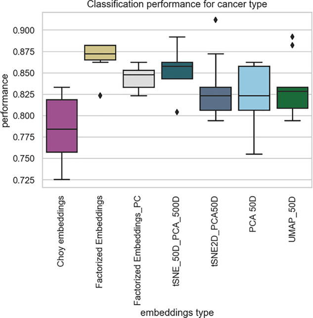
The FE-trained embeddings outperform all other representation in the prediction of cancer type task. We compared the representations of the FE model trained on all the data (FE) as well as an FE model trained on protein-coding genes only (FE_PC), to the downloaded weights for the Choy et al. model, a 50D t-SNE, a 2D t-SNE, a 50D UMAP and a 50D PCA. Each box and whiskers plot represents the performance of a five-nearest-neighbour classifier model tested on 20% of withheld data, reshuffled 100 times

Taken together, these results suggest that the FE model captures biologically relevant information in the sample representation.

3.8.1 The nature of gene embeddings

We then concentrated on the gene embeddings, to probe what kind of information might be captured by the FE model for individual genes. While sample embeddings offer a multitude of labels and categories, gene embeddings do not have this type of extensive categorization.

We compared side-by-side the gene embeddings obtained for the FE model to the weights provided by Choy et al. (2019) as well as Du et al. (2019). Both Du et al. and Choy et al. chose to train their models on a limited set of genes, mainly protein coding, and some microRNAs (24 447 and 20 531 genes, respectively). For the side-by-side comparison, we focused on protein-coding genes only, to mimic what was done by the other teams (Choy et al., 2019; Du et al., 2019).

We found that both the Choy and the FE models and to some extent the gene2vec model grouped genes by overall tissue specificity (Tau index) (Fig. 6, top row). However, we report that the FE model seems to aggregate genes by the maximal EMD for each tumour type (Fig. 6, middle row). Finally, for each gene, we selected the tumour type for which it is the most specific (see Section 3). We grouped tumours according to their tissue of origin and found that FE organizes genes by tissue specificity (Fig. 6, bottom row).

Fig. 6.

Gene embeddings trained with FE group tissue-specific genes. For the gene representations obtained for the Choy, Du and FE models, we calculated for each gene the Tau index of tissue specificity and a tissue-specific EMD (Section 3). Each point represents a gene and they are coloured by either Tau index or maximal EMD over all tissues. The bottom row shows genes coloured by the tissue, to which they are specific, obtained by taking the maximal argument over tissue specificities

Besides tissue specificity, gene–gene co-expression (measured by correlation) drives differential gene expression analyses. We found that correlated genes were located close-by in gene embedding space (Fig. 7). However, we found that proximity in location in the gene embedding space does not necessarily mean correlation in gene expression (Fig. 7).

Fig. 7.

FE groups correlated genes together in embedding space. For randomly selected pairs of genes at various correlation intervals, we measure the pair-wise Euclidean distance

Our final way of characterizing genes is their involvement in common cell processes. To probe the recovery of this gene feature, we selected a range of Gene Ontology terms (GO terms), by gene set size (Ashburner et al., 2000). The rationale is that the smaller the GO term gene set size, the more precise the GO term is. We hypothesize that if the gene embeddings capture gene participation in similar processes, it should group closer together genes participating in narrow GO terms and vice versa. We found that FE trained on GTEx but not the Choy nor the gene2vec embeddings preserve the relationship between GO term size and max Euclidean distance (Fig. 8). This may be at least in part attributed to the fact that the Choy model was trained on the TCGA cohort and Du et al. trained their model on an amalgam of GEO datasets. Indeed, the change in dataset drastically changes the recovery of the relationship (Fig. 8C and D). Taken together, our results show that the gene representations learned by the FE model capture both gene tissue specificity, co-expression patterns as well as cellular processes and gene type (Supplementary Material).

Fig. 8.

The FE-trained on GTEx gene representations capture GO term participation. We selected GO terms with increasing gene set size (and decreasing specificity) and calculated for each gene set the maximal intra-set distance in the various embedding spaces. We calculate a Pearson correlation coefficient for (A) Choy, (B) gene2vec (Du), (C) factorized embeddings trained on cancer samples and (D) FE trained on healthy tissues

3.9 Validation of the embeddings on auxiliary task

We believe that the nature of the RNA-Seq data offers a rich glimpse into cell processes that goes beyond just gene expression profiles. For example, mutations in some regions are reported to alter gene expression and therefore will leave an imprint of the transcriptome (Audemard et al., 2018). Moreover, Rappoport et al. report that their computational method performs in some cases best when trained on RNA-Seq data, compared to training on various multi-omics datasets (Rappoport and Shamir, 2018). In our work, we have shown that the embedding spaces learned by the FE model capture biologically meaningful information—on gene function and gene–gene co-expression, patient-specific gene expression as well as tissue-specific gene expression patterns. We wanted to validate the usage of the FE model as a dimensionality reduction method in a series of tasks that involve other types of assays. Conveniently, Thorsson et al. used the TCGA RNA-Seq data combined with microscopy, copy-number variant, whole genome sequencing and additional RNA-Seq data processing pipelines to characterize the tumours from an immunological point of view (Thorsson et al., 2018). We obtained from their work a total of 49 additional labels for the samples of the TCGA cohort. We grouped the labels by the nature of the additional data or algorithm that was required to obtain these labels. These groups are as follows:

• Cibersort refers to the prediction of infiltration of various immune cells obtained by the Cibersort algorithm (Newman et al., 2015).

• Thorsson immune profiles are the final immune profile categories specified by (Thorsson et al., 2018).

• Immune repertoire is a measure of B cell and T cell receptor diversity, requiring a special type of quantification done on bulk RNA-Seq (Bolotin et al., 2015).

• Genomic instability is a group of tasks that includes measures, such as incidence of synonymous and non-synonymous mutations, aneuploidy score, homologous recombination defects.

• Microscopy refers to tasks that require interpretation of microscopy images of tumour biopsies. Examples of such tasks are quantification of leukocyte fraction and stromal fractions and estimation of intra-tumoural heterogeneity.

We hypothesize that the sample embeddings trained by the FE model contain enough signal to perform on each of these 49 regression tasks. We compare the FE sample embeddings to the embeddings obtained by a 50-dimensional t-SNE, UMAP, PCA as well as a 2-dimensional t-SNE. For each task, we trained a kNN regressor model on 80% of the dataset and test on a held out 20%. This process was repeated a total of 100 times (Supplementary Material). Then, we grouped the tasks by the type of data and ranked performance-wise the various embeddings we compared (Fig. 9 A). We found that the FE model consistently ranked first performance-wise in 60% of the tasks overall and second in almost 40% (Fig. 9A). The second-best embedding was the 50-dimensional t-SNE that ranked first about 30% of the time and second almost 70% of the time (Fig. 9A). There is no clear distinction in the performance of the other three embeddings. We verified if the difference in performance is statistically significant when comparing FE to other embeddings using an ANOVA test, followed by a post hoc Tukey test. We report that the FE-trained sample embeddings outperformed all three UMAP50D, PCA50D and t-SNE2D almost 100% of the time (Fig. 9B). However, while the FE-trained embeddings ranked higher in performance, the difference was not always statistically significant when compared to the 50-dimensional t-SNE-trained embeddings (Fig. 9B)—notably, for the genomic instability task, none of the performances was statistically significant (Supplementary Material).

Fig. 9.

The FE representation of samples of the TCGA cohort outperforms in a series of 49 tasks all the other representations. (A) For every task group, we ranked the algorithms by performance and separated the tasks into task groups (Section 3). (B) For every task group, we showed the proportion of tasks where the FE embeddings outperformed each other representation (corrected P-value < 0.05, ANOVA followed by post hoc Tukey test). (C) An example of task group where the difference in performance between the FE representation and the others is statistically significant (P-value < 0.001)

We examined more closely one of these results, the immune repertoire task, where the FE-trained embeddings outperformed all other embeddings (Fig. 9B, bottom row and C). We suspect that the high performance of the FE-trained embeddings on this task is due to the link between the tumour type and the immune infiltration. Indeed, it has previously been reported that immune infiltration varies by tumour type, amongst other things (Thorsson et al., 2018; Iglesia et al., 2016). We therefore conclude that at least part of the good performance of the FE-trained embeddings stems from the performance at the easiest task—the tumour-type categorization (Fig. 5).

4 Discussion and conclusions

Together with the work of Choy, Shreiber and Du and colleagues, the FE model fits into a small family of self-supervised learning algorithms that perform tensor factorization of the dataset into separate latent spaces. We demonstrated the utility and performance of FE on two large-scale RNA-Seq cohort: TCGA and GTEx. When compared to the most similar model, published by Choy et al. (2019), we found that FE captures more biologically meaningful information in the sample and gene embeddings, which is probably due to the fact that the FE model but not the Choy model uses a set of fully connected layers on top of the embeddings layers. Unexpectedly, we found that the FE model preserves gene expression pair-wise distances in embedding space as well as being coherent with both single gene expressions across samples and more broad gene expression patterns. Moreover, we found it possible to perform the same type of vector-space arithmetics in sample embedding space as described in the works of Mikolov et al. (2013) and Pennington et al. (2014), transforming one tissue into the other, while preserving the patient-specific gene expression profile. This feature is something that non-parametric distance-based approaches, such as t-SNE, do not allow, since there is no way to reconstruct the data from the representation.

Finally, we demonstrated the utility of the encoding samples into a smaller, information-rich representation, by running a total of 49 benchmark tasks that involve predicting results from other assays on the same samples. We found that FE-trained representations rank mostly first and sometimes second and outperforms all the other dimensionality reduction algorithms on all 49 benchmarks. We found that in a small amount of cases, it is not statistically different from the performance of a 50-dimensional t-SNE. We would like to point out one of the possible limitations behind the performance of the benchmark experiments is that most of these labels are closely related to the tumour type and therefore some of the outstanding performance of the FE-trained embeddings may be attributable to this. Also, we were unable to identify gene categories standing out within the gene embedding space. This likely reflects the fact that most genes are multi-functional and involved in several processes across different tissue types and cancers. It is also unfortunate that very little categories are available for genes besides GO annotation, which are mostly derived from the study of healthy tissues. One possible extension would be to add some notion of gene function and/or localization that is available in the literature.

An appealing feature of the FE model is that it can, with little adjustments, be adapted to train on large-scale multi-omics datasets by introducing supplementary embedding spaces and jointly optimizing as many functions $g()$ (see Sections 2 and 3) as there are sources of observations, which could very well be additional clinical information on patients. Embeddings representing spaces shared by multiple data sources would be constrained to integrate these sources. This extension would naturally take advantage of the fact that our approach is not affected by missing data. Importantly, it would not require that datasets be complete, where all modalities would be measured for all samples. Furthermore, exploiting this later feature would support the use of the FE model for missing data imputation. More challenging would be the extension of the FE model to less ‘categorical’ spaces, a direction we have previously explored, in a limited context, by adapting the FE model to the work with transcript sequences instead of relying on a predefined transcriptome annotation (Trofimov et al., 2018). Non-trivial implementation issues, resulting in poor scalability of the proposed model, have so far limited its development.

We believe that the FE model is a highly customizable architecture that provides a strong foundation to develop omics-based predictors based on integrated data sources, resilient to missing data and provide similar benefits to other dimensionality reduction techniques in extracting patterns from omics data.

References

- Asgari E., Mofrad M.R.K. (2015) Continuous distributed representation of biological sequences for deep proteomics and genomics. PLoS One, 10, e0141287. [DOI] [PMC free article] [PubMed] [Google Scholar]
- Ashburner M. et al. (2000) Gene ontology: tool for the unification of biology. The Gene Ontology Consortium. Nat. Genet., 25, 25–29. [DOI] [PMC free article] [PubMed] [Google Scholar]
- Audemard E. O. et al. (2019) Targeted variant detection using unaligned RNA-Seq reads. Life Science Alliance, 2, e201900336. 10.26508/lsa.201900336 [DOI] [PMC free article] [PubMed] [Google Scholar]
- Bolotin D.A. et al. (2015) MiXCR: software for comprehensive adaptive immunity profiling. Nat. Methods.,12, 380–381 . [DOI] [PubMed]
- Bray N.L. et al. (2016) Near-optimal probabilistic RNA-seq quantification. Nat. Biotechnol., 34, 525–527. [DOI] [PubMed] [Google Scholar]
- Brunet J.-P. et al. (2004) Metagenes and molecular pattern discovery using matrix factorization. Proc. Natl. Acad. Sci. USA, 101, 4164–4169. [DOI] [PMC free article] [PubMed] [Google Scholar]
- Choy C.T. et al. (2019) Embedding of genes using cancer gene expression data: biological relevance and potential application on biomarker discovery. Front. Genet., 9, 682. [DOI] [PMC free article] [PubMed] [Google Scholar]
- Du J. et al. (2019) Gene2vec: distributed representation of genes based on co-expression. BMC Genomics, 20, 82. [DOI] [PMC free article] [PubMed] [Google Scholar]
- Gibbons F.D., Roth F.P. (2002) Judging the quality of gene expression-based clustering methods using gene annotation. Genome Res., 12, 1574–1581. [DOI] [PMC free article] [PubMed] [Google Scholar]
- Goldman M. et al. (2020) Visualizing and interpreting cancer genomics data via the Xena platform. Nat Biotechnol. 10.1038/s41587-020-0546-8 [DOI] [PMC free article] [PubMed]
- Gönen M. (2009) Statistical aspects of gene signatures and molecular targets. Gastroint. Cancer Res. 3(2 Suppl), 19–21. [PMC free article] [PubMed] [Google Scholar]
- Harris Z.S. (1954) Distributional structure. WORD, 10, 146–162. [Google Scholar]
- Iglesia M.D. et al. (2016) Genomic analysis of immune cell infiltrates across 11 tumor types. J. Natl. Cancer Inst., 108, djw144. [DOI] [PMC free article] [PubMed] [Google Scholar]
- Kim H., Kim Y.M. (2018) Pan-cancer analysis of somatic mutations and transcriptomes reveals common functional gene clusters shared by multiple cancer types. Sci. Rep., 8. [DOI] [PMC free article] [PubMed] [Google Scholar]
- Lemieux S. et al. (2017) MiSTIC, an integrated platform for the analysis of heterogeneity in large tumour transcriptome datasets. Nucleic Acids Res., 45, e122. [DOI] [PMC free article] [PubMed] [Google Scholar]
- Maciejewski H. (2014) Gene set analysis methods: statistical models and methodological differences. Brief. Bioinformatics, 15, 504–518. [DOI] [PMC free article] [PubMed] [Google Scholar]
- McInnes L. et al. (2018) UMAP: uniform manifold approximation and projection for dimension reduction. arXiv preprint arXiv:1802.03426
- Mikolov T. et al. (2013) Efficient estimation of word representations in vector space. arXiv preprint arXiv: 1301.3781v3
- Moon K.R. et al. (2019) Visualizing structure and transitions in high-dimensional biological data. Nat. Biotechnol., 37, 1482–1492. [DOI] [PMC free article] [PubMed] [Google Scholar]
- Murphy K.P. (2012) Machine Learning: A Probabilistic Perspective. MIT Press, Cambridge, MA. [Google Scholar]
- Newman A.M. et al. (2015) Robust enumeration of cell subsets from tissue expression profiles. Nat. Methods, 12, 453–457. [DOI] [PMC free article] [PubMed] [Google Scholar]
- Ng P. (2017) dna2vec: Consistent vector representations of variable-length k-mers. arXiv preprint arXiv:1701.06279.
- Paszke A. et al. (2019) PyTorch: an Imperative Style, High-Performance Deep Learning Library In: Wallach H.et al. (eds.) Advances in Neural Information Processing Systems. Vol. 32 Curran Associates, Inc, pp. 8024–8035. [Google Scholar]
- Pennington J. et al. (2014) GloVe: global vectors for word representation. In: Empirical Methods in Natural Language Processing (EMNLP), pp. 1532–1543. [Google Scholar]
- Rappoport N., Shamir R. (2018) Multi-omic and multi-view clustering algorithms: review and cancer benchmark. Nucleic Acids Res., 46, 10546–10562. [DOI] [PMC free article] [PubMed] [Google Scholar]
- Regev A. et al. (2017) The human cell atlas. eLife, 6. [DOI] [PMC free article] [PubMed] [Google Scholar]
- Roweis S.T., Saul L.K. (2000) Nonlinear dimensionality reduction by locally linear embedding. Science, 290, 2323‐2326. [DOI] [PubMed]
- Schreiber J. et al. (2020) Avocado: a multi-scale deep tensor factorization method learns a latent representation of the human epigenome. Genome Biol., 21, 81. [DOI] [PMC free article] [PubMed]
- Thorsson V. et al. (2018) The immune landscape of cancer. Immunity, 48, 812–830. [DOI] [PMC free article] [PubMed] [Google Scholar]
- Trofimov A. et al. (2018) Towards the latent transcriptome. arXiv preprint arXiv:1810.03442.
- Van Der Maaten L.J.P. et al. (2009) Dimensionality reduction: a comparative review. J. Mach. Learn. Res., 10, 1–41. [Google Scholar]
- Wagner A. et al. (2016) Revealing the vectors of cellular identity with single-cell genomics. Nat. Biotechnol., 34, 1145–1160. [DOI] [PMC free article] [PubMed] [Google Scholar]
- Yanai I. et al. (2005) Genome-wide midrange transcription profiles reveal expression level relationships in human tissue specification. Bioinformatics, 21, 650–659. [DOI] [PubMed] [Google Scholar]
Associated Data
This section collects any data citations, data availability statements, or supplementary materials included in this article.