TinGa: fast and flexible trajectory inference with Growing Neural Gas

Abstract

Motivation

During the last decade, trajectory inference (TI) methods have emerged as a novel framework to model cell developmental dynamics, most notably in the area of single-cell transcriptomics. At present, more than 70 TI methods have been published, and recent benchmarks showed that even state-of-the-art methods only perform well for certain trajectory types but not others.

Results

In this work, we present TinGa, a new TI model that is fast and flexible, and that is based on Growing Neural Graphs. We performed an extensive comparison of TinGa to five state-of-the-art methods for TI on a set of 250 datasets, including both synthetic as well as real datasets. Overall, TinGa improves the state-of-the-art by producing accurate models (comparable to or an improvement on the state-of-the-art) on the whole spectrum of data complexity, from the simplest linear datasets to the most complex disconnected graphs. In addition, TinGa obtained the fastest execution times, showing that our method is thus one of the most versatile methods up to date.

Availability and implementation

R scripts for running TinGa, comparing it to top existing methods and generating the figures of this article are available at https://github.com/Helena-todd/TinGa.

1 Introduction

Single-cell technologies have recently dramatically reshaped the landscape of techniques to model and better understand biological systems. Trajectory inference (TI) methods have recently emerged as a new category of unsupervised machine learning techniques to interpret single-cell data (Cannoodt et al., 2016). These methods aim to align cells along developmental trajectories, allowing researchers to get insight into the biological processes driving dynamic processes such as cell development and differentiation (Ji and Ji, 2016; Shin et al., 2015; Trapnell et al., 2014). More than 70 TI methods have been published up to date, differing in their methodologies, the input they need from the user and in the type of trajectories that they can model. Indeed, the first TI tools [Wanderlust, Bendall et al. (2014) and Monocle, Hill et al. (2015)] were able to model very simple linear trajectories. With new tools being generated, the complexity of the trajectories that could be modelled increased greatly, from branching [DPT, Haghverdi et al. (2016) and Wishbone, Setty et al. (2016)] or cycling [reCAT, Ye et al. (2019)], to more intricate graph structures [SLICER, Welch et al. (2016)].

Even though a large number of trajectory methods exist, the spectrum of topologies that can be modelled is unevenly distributed. A large number of the existing tools allow analysing simple linear trajectories. However, for more complex graph structures, there are only a handful of adequate methods. For the most complex topology considered in this article, that is trajectories that might consist of several disconnected components, only three existing methods can be applied: PAGA (Wolf et al., 2019), StemID (Grün et al., 2016) and Monocle 3 (Cao et al., 2019). In a recently published paper on TI, Saelens et al. (2019) compared 45 of the existing TI methods. Several interesting findings resulted from this study, including the strengths and weaknesses of existing tools as well as possible gaps in the field of TI. A first conclusion from this study was that no existing method was able to return accurate results for all the 350 datasets that were included in the study. Therefore, when facing a new unknown dataset, researchers need to apply several of the state-of-the-art methods and then compare their results in order to be able to gain biological insight into the data. It could be argued that the methods that can model the most complex trajectories could be applied in general, since they should also be able to model the simplest trajectories. However, a general observation made by the authors was that such methods then tend to be biased towards producing more complex trajectories in comparison to the ground truth. Therefore, when facing a new dataset with an unknown structure, there is still room for new methods that can deal with both simple and complex topologies in a flexible manner. Ideally, such methods would also be scalable, and able to run on datasets with millions of cells in an acceptable runtime.

2 Materials and methods

2.1 Adaptive topology modelling using Growing Neural Gas

In this article, we introduce TinGa, a fast and flexible TI method. It is the first method that applies the Growing Neural Gas algorithm [GNG, Fritzke (1995)] to infer trajectories. The basic idea behind this algorithm is to build a (possibly disconnected) graph that aims to fit a set of data points as well as possible using a graph structure that is iteratively adapted. The algorithm starts by building a graph that consists of two nodes, linked by an edge. An iterative procedure is then applied in which a random cell from the dataset is picked as input at every iteration and subsequently the graph is adapted to the data. An algorithmic description of TinGa is given in Algorithm 1. All nodes have an associated error that is representative of how well each node covers a certain region of the data space. A new node is added to the graph every λ iterations until a maximum number of nodes is reached. The new nodes are added close to the nodes with a maximal error, such that the graph grows until it covers the data homogeneously. The edges in the graph age if they are not stimulated by any input data, and die after they reach a certain age. The procedure results in a graph whose nodes and edges are representative of the data density structure.

After obtaining the graph structure using the GNG algorithm, putative noisy edges are cleared from this structure. The triangle structures in the graph are simplified by building a minimal spanning tree. However, this process can also remove edges that were representative of the data structure. A second post-processing step is therefore applied, in which nodes of degree one are identified. We then test if an edge should be added between pairs of nodes of degree one, following three rules:

1. the edge should exist in the GNG original result (before a minimal spanning tree was computed);

2. adding the new edge should not result in a triangle; and

3. the cell density along the new edge should be comparable to the mean density across the rest of the graph’s edges (which we defined as equal or superior to the mean density in the rest of the graph).

Algorithm 1: TinGa

1: input the matrix of reduced dimensions d

2: parameters max_iter, age_max, max_nodes, α, β, ϵ_b, ϵ_n, λ

3: procedure Compute a TinGa graph

4: initialise objects that will store information about the graph.:

5:  $\mathit{Nodes}\leftarrow \text{matrix}(\mathit{max}\_\mathit{nodes}\hspace{0.17em}\text{rows},\text{ncol}(d)\text{columns})$

6:  $\mathit{Edges}\leftarrow \text{list} \text{that} \text{will} \text{contain} \text{the} \text{TinGa} \text{edges}$

7:  Nodes error ← list that will contain the node associated errors

8:  Age edges ← matrix(max_nodes rows, max_nodes columns)

9: initialise graph with two cells.:

10:  $N\hspace{0.17em}\mathit{odes}[c(1,2),]\leftarrow .25\hspace{0.17em}\text{and}\hspace{0.17em}.75\hspace{0.17em}\text{quantiles}\hspace{0.17em}d$

11:  $\text{add} \text{edge} \text{of} \text{age} 0 \text{between} \text{nodes} 1 \text{and} 2$

12: while (iter < max_iter):

13:  $x_i\leftarrow \text{sample}\hspace{0.17em}\text{input}\hspace{0.17em}\text{cell}\hspace{0.17em}\text{in}\hspace{0.17em}d$

14:  $s_1,s_2\leftarrow 1\text{st} \text{and} 2\text{nd} \text{closest} \text{nodes} \text{to} x_i$

15:  $\text{increase} \text{age} \text{of} \text{all} \text{edges} \text{emanating} \text{from} s_1$

16:  $\text{add} \text{distance} (x_i-s_1) \text{to} \text{error} \text{of} s_1$

17:  $\text{Move} s_1 \text{towards} x_i\hspace{0.17em}\mathrm{a} \text{factor} {\mathrm{ϵ}}_b$

18:  $\text{Move} s_1^{\prime }\mathrm{s}\hspace{0.17em}\text{neighbors}\hspace{0.17em}\text{towards}\hspace{0.17em}{x}_i\hspace{0.17em}\mathrm{a} \text{factor} {\mathrm{ϵ}}_n$

19:  $\text{set} \text{age} \text{of} \text{edge} \text{between} s_1\hspace{0.17em}\text{and}\hspace{0.17em}{s}_2 \text{to} 0$

20:  if$\exists \hspace{0.17em}\text{edge}\hspace{0.17em}\text{of}\hspace{0.17em}\text{age}>\mathit{age}\_\mathit{max}$then

21:   $\text{remove} \text{it}$.

22:   if$\exists \text{node} \text{of} \text{degree} 0$then

23:    $\text{remove} \text{it}$.

24:  if$\text{iter} \% \lambda =0$then

25:   if$\text{number} \text{of} \text{nodes}<\mathit{max}\_\mathit{nodes}$then

26:    $p\leftarrow \text{node} \text{with} \text{maximum} \text{error}$.

27:    $q\leftarrow \text{neighbour} \text{of} p \text{with} \text{maximum} \text{error}$.

28:    $\text{insert} \mathrm{a} \text{new} \text{node} r \text{between} p \text{and} q$.

29:    $\text{errors} \text{of} p \text{and} q \text{are} \text{multiplied} \text{by} \alpha$

30:    $r \text{gets} \text{the} \text{mean} \text{error} \text{of} p \text{and} q$

31:    p–q edge is removed, p–r and r–q edges are added

32:  $\text{decrease} \text{error} \text{of} \text{all} \text{nodes} \text{by} \text{factor} \beta$

33: post-process the graph.:

34:  $\text{build} \mathrm{a} \text{graph} \text{from} \text{Nodes} \text{and} \text{Edges}$

35:  $\text{apply} \mathrm{a} \text{minimal} \text{spanning} \text{tree} \text{to} \text{the} \text{graph}$

36:  $\text{identify} \text{nodes} \text{in} \text{the} \text{MST} \text{of} \text{degree} 1$

37:  $\text{for} \text{each} \text{pair} \text{of} \text{nodes} p_1 \text{and} p_2 \text{of} \text{degree} 1\text{:}$

38:  if$\text{graph}\subseteq \text{edge} \mathrm{p}1-\mathrm{p}2$then

39:   if$\text{edge}\hspace{0.17em}\text{doesn}’\mathrm{t}\hspace{0.17em}\text{result}\hspace{0.17em}\text{in}\hspace{0.17em}\mathrm{a}\hspace{0.17em}\text{triangle}$then

40:    if$\text{cell} \text{density} \text{along} \text{edge} \text{is} \text{sufficient}$then

41:     $\text{add} \text{edge} \text{between} p_1 \text{and} p_2$.

An example of different iterations of the algorithm on a disconnected trajectory is shown in Figure 1. The fact that an error is attributed to every node in the graph helps to keep track of the data coverage. Nodes with high errors help to localize regions that are not sufficiently covered, in which new nodes will be added to help capture the region’s structure. Since the nodes are allowed to move towards the input that stimulated them, the GNG graph iteratively evolves to cover the density structure of the dataset. The fact that edges get removed if they get too old allows the graph to split, and not linger over empty regions.

Fig. 1.

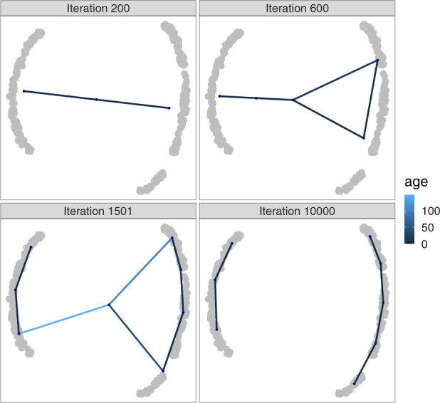
Different iterations of TinGa applied on a disconnected trajectory. The age of the graph edges is represented in different shades of blue to highlight edges that are getting old (in light blue) and are soon to be removed

2.2 Datasets

For this study, we used 350 datasets that were used in the benchmarking study described in Saelens et al. (2019), all of which have a known ground truth trajectory useful for evaluation. A large spectrum of topologies is represented in these datasets, from the simplest linear trajectories to the most complex disconnected trajectories. In Figure 2, each of the nine possible topology types is represented as a graph. In bifurcations, a simple linear trajectory bifurcates into two branches. Converging trajectories are the exact opposite of bifurcations: two distinct branches merge into one. Trees consist of a succession of different bifurcations. Multi-furcations happen when a simple linear branch splits into more than two branches. Finally, some of the datasets are graphs; they can contain cycles or be acyclic, depending on the direction along the branches.

Fig. 2.

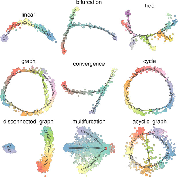
Examples of the possible trajectory topologies. In each graph, the ground truth trajectory is represented by oriented lines, separated by nodes. The cells are coloured based on the node to which they are closest

We have split the 350 datasets in two. Table 1 describes the 100 out of 350 datasets that were used for testing TinGa’s robustness to its parameter setting, and fine-tuning of the max_nodes parameter. We then used the remaining 250 datasets to compare TinGa to 4 other TI methods. These 250 datasets contained 9 different types of trajectories, as can be seen in Table 2. Both the 100 datasets used for parameter tuning as well as the 250 datasets used for benchmarking to other methods contained comparable numbers of real and synthetic datasets. The synthetic datasets were generated using four simulators: dyngen (Saelens et al., 2019), which simulates gene regulatory networks, dyntoy (Saelens et al., 2019), which builds random gradients of expression in the reduced space, PROSSTT (Papadopoulos et al., 2019), which samples the expression from a linear model that depends on pseudotime and Splatter (Zappia et al., 2017), which simulates non-linear paths between different expression states. In total, 240 synthetic datasets were thus generated using these four simulators. The cells in each dataset were then post-processed to match a real dataset’s characteristics such as the dropout rate. Combined with 110 real datasets, this thus resulted in the total number of 350 datasets, split in a set of 100 datasets for parameter tuning and 250 datasets for benchmarking to other TI methods.

Table 1.

Datasets used for parameter tuning

Trajectory type	Real datasets	Synthetic datasets	Total datasets
Linear	18	4	22
Cyclic	0	6	6
Bifurcating	6	10	16
Converging	1	5	6
Multi-furcating	1	1	2
Tree	8	23	31
Acyclic graph	0	3	3
Connected graph	0	7	7
Disconnected graph	4	3	7
Total	38	62	100

Table 2.

Datasets used to evaluate the methods

Trajectory type	Real datasets	Synthetic datasets	Total datasets
Linear	21	26	47
Cyclic	2	21	23
Bifurcating	7	21	28
Converging	0	11	11
Multi-furcating	8	6	14
Tree	11	45	56
Acyclic graph	1	13	14
Connected graph	0	28	28
Disconnected graph	22	7	29
Total	72	178	250

2.3 Single-cell RNA-seq data preprocessing

Real datasets were preprocessed following the standard bioconductor pipeline which uses both the scran and scater Bioconductor packages(Amezquita et al., 2020; Lun et al., 2016). The same settings were used as in Saelens et al. (2019), with a filtering that removed genes that were expressed in less than 5% of the cells and had an average expression lower than 0.02. Cell filtering was applied based on total counts, total amount of features, mitochondrial gene expression and if available, spike-ins, where cells with values higher than the median ± 3 MADs were removed. The most highly variable genes were selected by modelling the mean–variance relationship with a curve, and identifying genes that differed from this curve with a false discovery rate of 5% and a biological component (or effect size) higher than 0.5, using the scran R package.

2.4 Benchmarking TinGa to state-of-the-art methods

We compared TinGa to four top TI methods, as identified by the large-scale benchmarking study by Saelens et al. (2019). These are Slingshot (Street et al., 2018), PAGA (Wolf et al., 2019), RaceID/StemID (Grün et al., 2016) and Monocle 3 (Cao et al., 2019). Since the dynbenchmark package (Saelens et al., 2019) contained wrappers for most of these methods, metrics for comparison, as well as 110 real and 240 synthetic datasets on which we could compare the methods, we re-used the same comparison settings. We created one new wrapper for Monocle 3, a method that was not yet included in the dynbenchmark package. Four metrics, earlier described in Saelens et al. (2019), were used to assess the performance of the method:

• Hamming–Ipsen–Mikhailov (HIM): provides information on the difference in topology between a method’s result and a gold standard, by taking into account both the edge lengths and the similarity in node degrees

• CORRELATION: provides information on the correlation between the cell ordering in a method’s results compared to a gold standard, taking the trajectory structure into account by using geodesic distances.

• F1 BRANCHES: provides information on the difference in branch assignment between a method’s result and a gold standard

• FEATURE IMPORTANCE: provides information on the genes that are differentially expressed along a method’s result trajectory compared to a gold standard

Finally, we used a last metric, the MEAN SCORE, which is the geometric mean of the four aforementioned metrics.

2.5 TinGa parameter settings

We used the default parameters of GNG as described in Fritzke (1995). To test the applicability of each parameter setting, we performed a grid search for each parameter separately by varying the parameter over a large range of values while keeping the other parameters at their default value. These parameter values are as follows:

• $\mathit{max}\_\mathit{iter}$: the maximum number of iterations. Default: 10 000. No grid search was performed on this parameter, as the GNG has mostly converged after 10 000 iterations.

• ϵ_b: how much the closest node will move towards the input cell. Default: 0.05. Grid search was performed on values varying from 0.005 to 1.

• ϵ_n: how much the neighbours of the closest node will move towards the input. Default: 0.001. Grid search was performed on values varying from 0.0001 to 1.

• λ: the iteration at which a new node can be added. Default: 200. Grid search was performed on values varying from 100 to 500.

• $\mathit{age}\_\mathit{max}$: the maximum age of an edge before it is removed. Default: 200. Grid search was performed on values varying from 100 to 500.

• α: the decay parameter for error when a new node is added. Default: 0.5. Grid search was performed on values varying from 0.1 to 0.9.

• β: the value by which all node errors decrease at every iteration. Default: 0.99. Grid search was performed on values varying from 0.2 to 0.999.

• $\mathit{max}\_\mathit{nodes}$: the maximum number of nodes allowed in the GNG graph. Default: 30. Grid search was performed on values varying from 4 to 30.

We tested every resulting parameter setting on 100 randomly sampled datasets among the 350 datasets described in Saelens et al. (2019), which we used as our training set. We then performed paired t-tests to assess whether the mean score of TinGa over the 100 training datasets would change significantly due to parameter tuning. Varying the parameters α, β, λ and $\mathit{age}\_\mathit{max}$ did not significantly change the results of TinGa over these datasets (with a P-value of 0.05). We noticed that setting too high ϵ_b and ϵ_n values decreased the performance of TinGa, and we therefore advise to keep the values of these parameters equal to or lower than 0.5 and 0.01 for the ϵ_b and ϵ_n parameters, respectively. We believe that the fact that GNG nodes should not be allowed to move excessively under the influence of one cell input makes sense, since this allows the method to be more robust to outlier cells.

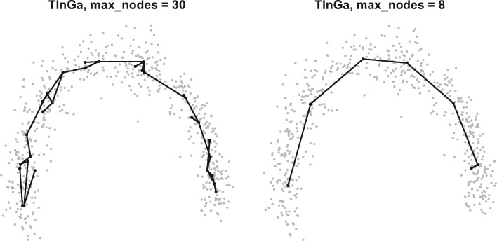
The only parameter whose default value showed sub-optimal results was the $\mathit{max}\_\mathit{nodes}$ parameter. The GNG algorithm was originally designed to learn complex topologies, and the default number of nodes in the graph was set to a relatively high value (with a maximum of 30 nodes). In the context of TI, this number seems inappropriate, as allowing too many nodes in the graph can lead to the appearance of noisy structures, as can be seen in Figure 3. We tested various values for the $\mathit{max}\_\mathit{nodes}$ parameter, ranging from 4 to the default of 30. The results of TinGa on the 100 datasets that we selected for training with different $\mathit{max}\_\mathit{nodes}$ values can be seen in Figure 4. We observed that a maximum number of eight nodes was a good trade-off between performance, as assessed by the mean score in the figure, and running time. We set the $\mathit{max}\_\mathit{nodes}$ parameter to eight and all other TinGa parameters to their default value for the rest of the study.

Fig. 3.

The trajectories identified by TinGa on a linear dataset. Even though the global structure of the data is captured in both examples, a total of 30 nodes seems to be too high and leads to a noisy trajectory, whereas 8 nodes seem sufficient to return a clean trajectory

Fig. 4.

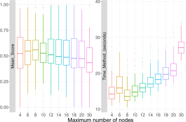
Result of the max_nodes parameter tuning. For each max_nodes value, we represented the mean score over 100 train datasets and the time it took to the method to run in seconds

All TI methods use low-dimensional data as input. In the case of TinGa, we reduced the dimensionality of the count matrix of synthetic and real datasets to five dimensions using multi-dimensional scaling. In order to test the robustness of TinGa’s results to the choice of the number of dimensions in the lower space, we tested different numbers ranging from 3 to 50, on the same 100 datasets we had already used for grid search on TinGa’s parameters. The number of dimensions didn’t have a high impact on TinGa’s results, as can be seen in Figure 5. To confirm this, we performed paired t-tests to assess whether the number of dimensions that we selected would change the results of TinGa with regards to other methods. The P-values associated with these tests were all higher than 0.05. TinGa is therefore robust to the number of dimensions in the data, and we fixed this number to 5 for the rest of the study. Dimensionality reduction was applied as defined by default by the authors for the four other TI methods that we tested.

Fig. 5.

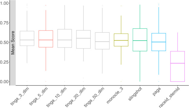
The mean score of four state-of-the-art methods, TinGa with the default number of dimensions = 5, and four other settings for this parameter, on 100 train datasets. The five original methods are represented in colour, the four versions of TinGa with different numbers of dimensions are in gray

3 Results

We compared the performance of TinGa to a set of state-of-the-art methods for TI, namely PAGA, Slingshot, RaceID/StemID and Monocle 3. The performance of all five methods was assessed on 250 synthetic and real datasets offering a wide variety of complexities, from linear to disconnected trajectories. For each of these datasets, the ground truth trajectory is known, since it was either defined experimentally for the real datasets, or extracted from simulations for the synthetic datasets. Therefore, the results of any TI method can be compared to the ground truth trajectory and scored. We performed a comparison using four metrics that we described in Section 2. We report the results of the methods on the 178 synthetic and 72 real datasets separately.

3.1 Synthetic datasets

TinGa and Slingshot are the methods that found the best cell ordering across all synthetic datasets, as shown by the correlation scores (Fig. 6a). These two methods also found the best cell assignment across branches (Fig. 6b). However, Monocle 3 performed better than Slingshot for recovering the topology of the datasets and the features expressed along the trajectory, as can be seen in the boxplots showing the Feature Importance score and the HIM score in Figure 6c and d, respectively. TinGa, on the other hand, was consistently among the best methods for these four metrics when applied on the synthetic datasets. The scores of RaceID/StemID were greatly affected by the fact that it failed to return results on many datasets. In order to make the comparison of five methods on 250 datasets possible, we set a maximum memory use of 15 Gb for every method on every dataset. RaceID/StemID systematically ran out of memory on datasets containing more than 5000 cells. Figure 6f shows the time each method took to run on the datasets in function of the number of cells. All methods returned results in less than 10 s on datasets containing less than 1000 cells, except for RaceID/StemID, which already needed a few minutes on a dataset of 1000 cells. TinGa proved to be very scalable on larger datasets, while Slingshot and PAGA became significantly slower on datasets containing a few thousands of cells. Overall, the TinGa method obtained the best scores when compared to the four currently state-of-the-art TI methods on synthetic datasets, as can be seen in Figure 6e, where the Mean Score is the geometric mean of the four other metrics (Correlation, F1 Branches, HIM and Feature_Importance). We performed statistical tests to assess if TinGa’s mean score was significantly higher than the mean scores of the four other methods on the different trajectory types. The P-values associated with these one-sided t-tests can be seen in Table 3, which contains P-values associated with paired t-tests computed on the 178 synthetic datasets. TinGa consistently performed significantly better than RaceID/StemID across all trajectory types. It also significantly outperformed Monocle 3 and PAGA on simpler trajectories such as linear, bifurcating, converging and cycles. On the other hand, the mean scores of TinGa were significantly higher than the mean scores of Slingshot on more complex trajectories such as trees and acyclic graphs (with a P-value of 0.05).

Fig. 6.

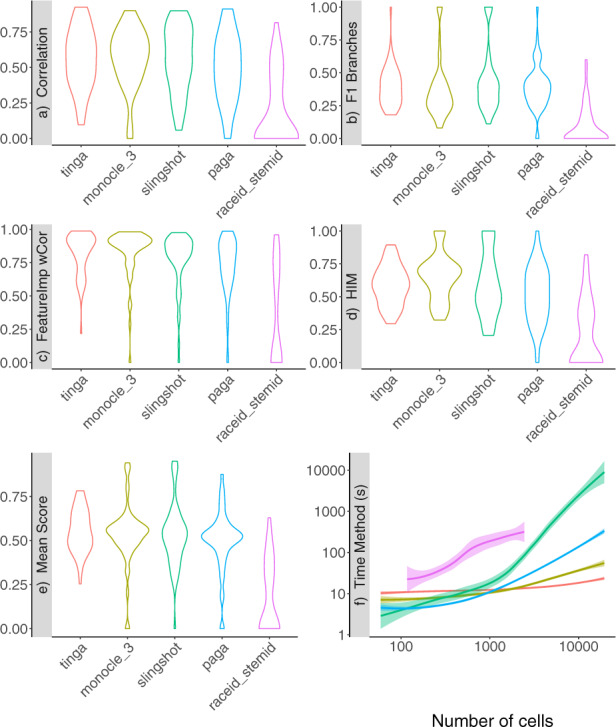
Scores of TinGa and five top TI methods applied on 178 synthetic datasets. The methods are ordered decreasingly with the mean score along the x-axis across the whole figure. (a) The correlation between the cell ordering in a method’s result and the ground truth. (b) The accuracy in branch assignment for the cells in a method’s result compared to the ground truth. (c) The ability of a method to recover the main features that drive the trajectory. (d) The accuracy of the recovered topology compared to the ground truth. (e) The mean score: mean of the four previous scores. (f) The time every method took on datasets of differing numbers of cells (from less than 500 cells to 10 000 cells), in seconds. We represented the time on the y-axis on a log scale, so that differences between methods that were fast on large datasets such as TinGa and Monocle 3 could be seen

Table 3.

P-values associated with one-sided paired t-tests assessing whether TinGa performed significantly better than the other methods on the different trajectory types

Trajectory type	Monocle 3	Slingshot	PAGA	RaceID/StemID
Linear	0.004	0.433	0.005	0
Cyclic	0	0.016	0	0
Bifurcating	0.011	0.297	0.037	0
Converging	0.002	0.062	0.003	0
Multi-furcating	0.104	0.546	0.495	0.005
Tree	0.742	0	0.356	0.001
Acyclic graph	0.210	0.007	0.204	0.001
Connected graph	0.942	0.163	0.064	0.001
Disconnected graph	0.597	0.086	0.806	0.006

For each of the 178 synthetic datasets, we determined which of the five tested methods performed the best. The results are presented in Figure 7. TinGa had the best score on 68 out of the 178 datasets. We also observed that TinGa was the method that performed best on the greater diversity of synthetic trajectory types. Monocle 3, the second-best method that outperformed the other methods on 42 synthetic datasets, mainly showed its best performance in two types of trajectories: trees and graphs. Slingshot, the third-best method that outperformed the others on 28 synthetic datasets, mainly outperformed the other methods on simpler trajectories, from linear to cycles, while PAGA and RaceID/StemID performed best on trees. On the other hand, TinGa outperformed the other methods on linear, bifurcating, cyclic, tree, acyclic and graph trajectories.

Fig. 7.

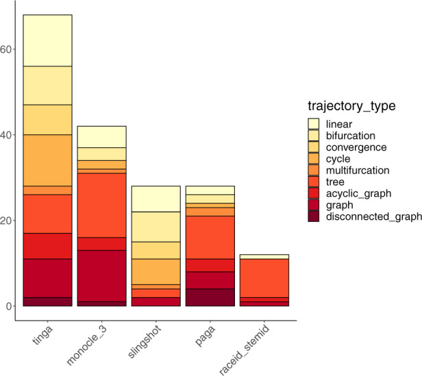
Methods on the x-axis are ordered by the number of datasets on which they outperformed the others. The y-axis represents the number of datasets on which each method had the best mean score across all methods. For each method, bars represent the different trajectory types for which the method performed best. These bars are ordered and coloured from most simple (in light yellow) to most complex trajectory type (in dark red)

3.2 Real datasets

Figure 8 shows violin plots of the scores of the five TI methods we tested on real datasets. These results were split between datasets with a silver and a gold standard. Datasets with a gold standard are datasets for which external information such as cell sorting or cell mixing were used for validation of the trajectory. In datasets with a silver standard, the ground truth trajectory was extracted directly from the expression data, typically by clustering and validation by experts.

Fig. 8.

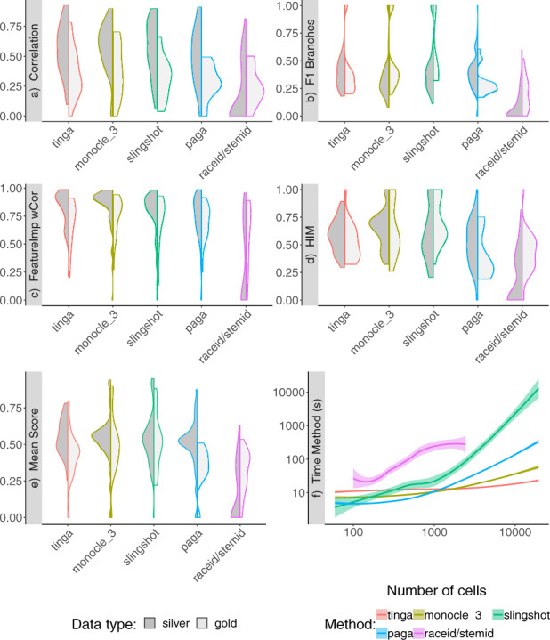
(a–e) The results on 54 datasets with a silver standard and 18 datasets with a gold standard were represented separately in split violin plots. (a) The correlation between the cell ordering in a method’s result and the ground truth. (b) The accuracy in branch assignment for the cells in a method’s result compared to the ground truth. (c) The ability of a method to recover the main features that drive the trajectory. (d) The accuracy of the recovered topology compared to the ground truth. (e) The mean score: mean of the four previous scores. (f) The time every method took on datasets of differing numbers of cells (from 60 cells to 19 647 cells), in seconds

In datasets with a silver standard, we observed results that were comparable to the results previously shown on synthetic datasets. TinGa, Slingshot, Monocle 3 and PAGA were the methods that had the best correlation and F1 branches scores, as can be seen in Figure 8a and b, respectively. As observed previously, Monocle 3 outperformed Slingshot on the feature importance score (Fig. 8c). In the case of datasets with a silver standard, it not only performed better than Slingshot but also TinGa and PAGA on the topology HIM score (Fig. 8d). Overall, the mean scores of TinGa and Slingshot were relatively spread from mediocre (0.25) to very good scores (>0.8) compared to Monocle 3 and PAGA, which returned more consistently mean scores around 0.55 on the real datasets with a silver standard. As observed on synthetic datasets, the scores of RaceID/StemID were greatly affected by the fact that it failed to return results on the large datasets, due to memory issues.

We compared the time necessary for each method to run (Fig. 8f). TinGa was the fastest of the five TI tools. It took 11 s on average to run on small datasets and only 21 s on average on datasets containing more than 10 000 cells. Monocle 3 had very similar results on small datasets, but it took twice longer than TinGa on our largest datasets. Moreover, the method crashed on nine datasets. PAGA took slightly more time to run on large datasets, needing more than 3 min on average to run on datasets containing more than 10 000 cells. This method did not work on all datasets either: it crashed on 17 of them. RaceID/StemID was the second slowest method and already needed a few minutes to run on medium datasets. This method systematically crashed on datasets of more than 5000 cells, which represents 69 datasets. Slingshot and TinGa were the only methods that returned a result for all the 250 real and synthetic datasets on which they were tested. However, Slingshot was the least scalable of the five methods that we tested, and ran for more than 2 h when applied to the largest dataset of the study that contained 19 647 cells. In comparison, TinGa took 23 s on the same dataset.

All methods performed significantly worse on datasets with a gold standard compared to silver-standard datasets. Since the validation of these trajectories does not rely on the data itself but on external measures, it might not reflect the processes in the data exactly and be more complex to infer. Even though Slingshot and Monocle 3 returned significantly lower correlation and featureimp_wcor scores than on the real datasets with a silver standard (Fig 8a and c), these two methods had the highest mean scores on datasets with a gold standard (Fig. 8e). The mean score of TinGa on these datasets was slightly lower than its results on silver and synthetic datasets, and the mean score of PAGA completely dropped on these datasets, never reaching a value higher than 0.5. This might in part be explained by the fact that datasets with a gold standard consisted mainly of linear and bifurcating trajectories, two trajectory types on which Slingshot tends to excel, while PAGA can over-estimate these datasets complexity (see Fig. 9).

Fig. 9.

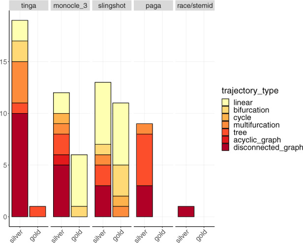
The results for the five methods are represented in separate plots along the x-axis. The y-axis represents the number of datasets on which each method had the best mean score on real datasets across all methods. These results are split into two bars, representing the results on real datasets with a silver and a gold standard separately. For each method, bars represent the different trajectory types for which the method performed best. These bars are ordered and coloured from most simple (in light yellow) to most complex trajectory type (in dark red)

The number of real datasets on which each method performed best are presented in Figure 9, where results on datasets with a silver and a gold standard are shown separately. TinGa outperformed the other methods on 18 silver-standard datasets, which ranged from simple linear to most complex disconnected trajectories. As observed previously in synthetic datasets, PAGA performed best on a majority of tree trajectories. Slingshot and Monocle 3 returned the best results on 16 and 14 real silver-standard datasets, respectively. These two methods also performed best on a majority of the simple real datasets with a gold standard, while TinGa performed best on the only real complex dataset with a gold standard.

We then performed statistical tests on the real datasets to assess whether TinGa’s mean score was significantly higher than the mean scores of the four other methods on any trajectory types. Table 4 shows the results of the one-sided paired t-tests that we performed, and contains the P-values computed among the real datasets. Since there was only one real dataset containing an acyclic graph, we could not compute any statistics on this trajectory type. As observed previously in synthetic datasets, TinGa consistently performed significantly better than RaceID/StemID across all trajectory types, except for real cyclic datasets. Moreover, the mean scores of TinGa were significantly higher than the mean scores of PAGA on both cyclic and linear datasets, and higher than the scores of Slingshot on the more complex trees and disconnected graphs (with a P-value of 0.05).

Table 4.

P-values associated with one-sided paired t-tests comparing TinGa to other methods on real datasets

Trajectory type	Monocle 3	Slingshot	PAGA	RaceID/StemID
Linear	0.913	0.986	0	0
Cyclic	0.761	0.811	0.042	0.217
Bifurcating	0.378	0.635	0.119	0.021
Multi-furcating	0.189	0.439	0.143	0
Tree	0.441	0.021	0.716	0
Acyclic graph	—	—	—	—
Disconnected graph	0.055	0	0.057	0

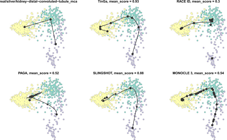
Figure 10 is shown as an example of the trajectories returned by the different methods on a real linear dataset. On this dataset, TinGa and Slingshot accurately retrieved a linear trajectory that was similar to the real trajectory (at the top left of the figure). The cell ordering was therefore optimally retrieved by these two methods, while PAGA for instance found a trajectory that diverged greatly from the ground truth, and reordered the cells in a very different way. The trajectory identified by Monocle 3 consists of many nodes, and even though it globally resembles the ground truth, it identified two noisy micro-structures: a branch and a cycle. In this case, the mean score of Monocle 3 was therefore impacted by the fact that the topology it returned was more complex than expected, which resulted in a low HIM score. It also suffered from the fact that some cells were assigned to an extra branch and an extra cycle that were not present in the ground truth trajectory, which resulted in a bad F1_branches score. RaceID/StemID and PAGA also returned a trajectory that was much more complex than the ground truth.

Fig. 10.

Trajectories found by the different methods on a real dataset with a linear trajectory. The mean score of each method reflects the accuracy with which it inferred the trajectory compared to the gold standard, which is represented in the top-left figure. TinGa and Slingshot inferred the most accurate trajectories on this dataset

3.3 Topology bias

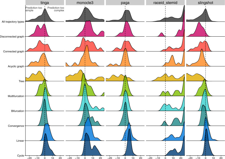
In order to further investigate the type of trajectory topology that TinGa would return compared to other methods, we then focused on the bias in topology. Saelens et al. (2019) had already highlighted the fact that some TI methods such as PAGA, tended to over-estimate the complexity of a trajectory, while other methods, amongst which Slingshot, typically under-estimated the complexity of a dataset. We assessed the difference in topology between the trajectories returned by the five TI methods tested in this article and the real data topologies (Fig. 11). Our results confirmed that PAGA, and also RaceID/StemID returned too complex trajectories when facing linear or cyclic datasets. We observed the same trend in Monocle 3, which also tends to reconstruct too complex topologies on linear or cyclic datasets. We also observe that RaceID/StemID tends to return extremely complex trajectories compared to ground truth, irrespective of the real topology in the data. On the other hand, slingshot and TinGa accurately returned linear topologies when facing simple datasets. We report however that Slingshot tends to model cyclic trajectories as linear, an error that TinGa typically circumvents.

Fig. 11.

The bias between the topology returned by a method and the ground truth topology is represented for each trajectory type (represented in rows), and for each method (represented in columns). This bias was computed as the difference in the number of nodes + the number of edges in the graph returned by a method compared to the ground truth. The dotted vertical lines represent a perfect match between a method’s and the ground truth topologies. The fact that a method’s results are on the right of the dotted line show us that this method tends to return too complex topologies compared to the real topology. Conversely, methods for which we observe results on the left of the dotted line tend to return too simple topologies

If we then focused on more complex datasets, such as converging, bifurcating or multi-furcating trajectories, we noticed that TinGa, PAGA and Slingshot were relatively unbiased towards the topology complexity. Monocle 3 and RaceID/StemID, on the contrary, tended to return overly complex trajectories for these topologies. Finally, if we focused on the most complex datasets on which we performed our comparison, we noticed that methods that tended to find too complex topologies in simple datasets performed more accurately on complex datasets. PAGA showed no bias in topology on disconnected graphs and showed only a slight bias in the direction of more simple topologies when applied to connected or acyclic graphs. Slingshot, on the other hand, under-estimated the complexity of disconnected, connected, acyclic and tree graphs. We observed the same trend in TinGa for the two last-mentioned topologies, but the bias was much less pronounced that the bias observed for Slingshot. All methods seemed to struggle with finding the right topology for tree datasets.

4 Discussion

So far, every new TI method that was published compared its results to a maximum of 10 other methods (which were not necessarily selected among the best ones), on a maximum of 10 datasets. In this work, we presented an extensive comparison of TinGa to four of the best existing TI methods to our knowledge on 250 datasets. This allowed us to clearly establish the relative performance of each method in a minimally biased setting, since adding more datasets automatically reduces the possibility that we would over-estimate the performance of our method. The datasets on which we tested TI methods were either generated by one of four different simulators or real single-cell RNA-seq datasets. This allowed us to test different aspects of the methods. In synthetic datasets, we have the advantage of having a refined gold standard, with information on every cell’s state of progression in the trajectory we simulated. Testing the methods on real datasets is of course essential, but in these datasets, a gold standard is more difficult to extract, and is usually based on a grouping of cells into time points or clusters, which is less refined than the single-cell information obtained in synthetic datasets.

The TinGa method showed a very good performance on average on all types of trajectories, while we observed that Slingshot performed best on simple trajectory types, and PAGA and Monocle 3 were more prone to reconstructing complex trajectories types.

Slingshot relies on two steps of first clustering the low-dimensional data and then fitting principal curves through these clusters. This results in the Slingshot trajectory typically being very well correlated with the gold-standard trajectory, since it follows the principal density structures in the data. However, this method also tends to smooth out the trajectory, possibly removing secondary structures such as branches or cycles. PAGA also starts with a clustering step, but the method then significantly differs from Slingshot since one small graph is then built per cluster. Several steps of refinement then allow linking the subgraphs that need to be linked while keeping separate the components that should not be merged, which allows the method to recover disconnected trajectories. This approach typically leads to more convoluted trajectories. Monocle 3 has a similar approach to PAGA, since it also performs clustering followed by a step where a principal graph is built for each cluster. Several refinement steps are then applied in order to produce a clean final graph, among which merging the subgraphs that should be linked. From what we observed in Figure 11, the similarities between PAGA and Monocle 3’s methodologies are reflected in the way they model simple trajectories, since they both tend to return more complex trajectories than needed when applied on linear or cyclic datasets. TinGa models the trajectory as a growing graph that naturally migrates towards the higher density regions in the data. It is comparable to Slingshot in the sense that it will approximate a principal curve’s result on simple trajectories. However, it also matches the best aspects of PAGA and Monocle 3 since it will eventually divide into subgraphs if the data are disconnected. From what we observed, TinGa seems to be a good trade-off between Slingshot, which is a method that performs optimally on simple trajectory types such as linear or bifurcating trajectories, and PAGA and Monocle 3, which perform best on graphs and trees but tend to return too complex topologies when facing simple trajectories. TinGa does not need the user to specify any topology. We reasoned that the fact that it can fit any topological structure in a scalable way with the number of inputs presented a real advantage in the context of TI.

In this setting, we observed that TinGa was a promising TI method. Its performance is comparable to Slingshot on simple datasets, but also accurate on complex trajectories where it performed equally well and sometimes outperformed the PAGA and Monocle 3 methods. In a field as complex as is TI, we believe that more than one TI tool should be used at the same time, to increase understanding of the data. We provide TinGa, a method that is applicable to a wide range of trajectory types, and can play a role in the inference of complex disconnected trajectories, a problem that very few methods are able to tackle for now, while still being accurate on simple trajectories.

Funding

Y.S. is an ISAC Marylou Ingram scholar. This research received funding from the Flemish Government under the ‘Onderzoeksprogramma Artificiële Intelligentie (AI) Vlaanderen’ programme.

Conflict of Interest: none declared.

References

- Amezquita R.A. et al. (2020) Orchestrating single-cell analysis with Bioconductor. Nat. Methods, 17, 137–145. [DOI] [PMC free article] [PubMed] [Google Scholar]
- Bendall S.C. et al. (2014) Single-cell trajectory detection uncovers progression and regulatory coordination in human b cell development. Cell, 157, 714–725. [DOI] [PMC free article] [PubMed] [Google Scholar]
- Cannoodt R. et al. (2016) Computational methods for trajectory inference from single-cell transcriptomics. Eur. J. Immunol., 46, 2496–2506. [DOI] [PubMed] [Google Scholar]
- Cao J. et al. (2019) The single-cell transcriptional landscape of mammalian organogenesis. Nature, 566, 496–502. [DOI] [PMC free article] [PubMed] [Google Scholar]
- Fritzke B. (1995) A growing neural gas network learns topologies. Adv. Neural Inform. Process. Syst., 7, 625–632. [Google Scholar]
- Grün D. et al. (2016) De novo prediction of stem cell identity using single-cell transcriptome data. Cell Stem Cell, 19, 266–277. [DOI] [PMC free article] [PubMed] [Google Scholar]
- Haghverdi L. et al. (2016) Diffusion pseudotime robustly reconstructs lineage branching. Nat. Methods, 13, 845–848. [DOI] [PubMed] [Google Scholar]
- Hill C. et al. (2015) Pseudo-temporal ordering of individual cells reveals dynamics and regulators of cell fate decisions. Proc. SPIEInt. Soc. Opt. Eng., 73, 389–400. [Google Scholar]
- Ji Z., Ji H. (2016) TSCAN: pseudo-time reconstruction and evaluation in single-cell RNA-seq analysis. Nucleic Acids Res., 44, e117. [DOI] [PMC free article] [PubMed] [Google Scholar]
- Lun A. et al. (2016) A step-by-step workflow for low-level analysis of single-cell RNA-seq data [version 1; referees: 5 approved with reservations]. F1000Res., 5, 2122. [DOI] [PMC free article] [PubMed] [Google Scholar]
- Papadopoulos N. et al. (2019) PROSSTT: probabilistic simulation of single-cell RNA-seq data for complex differentiation processes. Bioinformatics, 35, 3517–3519. [DOI] [PMC free article] [PubMed] [Google Scholar]
- Saelens W. et al. (2019) A comparison of single-cell trajectory inference methods. Nat. Biotechnol., 37, 547–554. [DOI] [PubMed] [Google Scholar]
- Setty M. et al. (2016) Wishbone identifies bifurcating developmental trajectories from single-cell data. Nat. Biotechnol., 34, 637–645. [DOI] [PMC free article] [PubMed] [Google Scholar]
- Shin J.Y. et al. (2015) Single-cell RNA-seq with waterfall reveals molecular cascades underlying adult neurogenesis. Cell Stem Cell, 17, 360–372. [DOI] [PMC free article] [PubMed] [Google Scholar]
- Street K. et al. (2018) Slingshot: cell lineage and pseudotime inference for single-cell transcriptomics. BMC Genomics, 19, 16. [DOI] [PMC free article] [PubMed] [Google Scholar]
- Trapnell C. et al. (2014) The dynamics and regulators of cell fate decisions are revealed by pseudotemporal ordering of single cells. Nat. Biotechnol., 32, 381–386. [DOI] [PMC free article] [PubMed] [Google Scholar]
- Welch J.D. et al. (2016) SLICER: inferring branched, nonlinear cellular trajectories from single cell RNA-seq data. BioMed Central, 17, 106. [DOI] [PMC free article] [PubMed] [Google Scholar]
- Wolf F.A. et al. (2019) PAGA: graph abstraction reconciles clustering with trajectory inference through a topology preserving map of single cells. Genome Biol., 20, 9. [DOI] [PMC free article] [PubMed] [Google Scholar]
- Ye Y. et al. (2019) Circular trajectory reconstruction uncovers cell-cycle progression and regulatory dynamics from single-cell Hi-C maps. Adv. Sci., 6, 1900986. [DOI] [PMC free article] [PubMed] [Google Scholar]
- Zappia L. et al. (2017) Splatter: simulation of single-cell RNA sequencing data. Genome Biol., 18, 174. [DOI] [PMC free article] [PubMed] [Google Scholar]