

Abstract
Motivation
The universal expressibility assumption of Deep Neural Networks (DNNs) is the key motivation behind recent worksin the systems biology community to employDNNs to solve important problems in functional genomics and moleculargenetics. Typically, such investigations have taken a ‘black box’ approach in which the internal structure of themodel used is set purely by machine learning considerations with little consideration of representing the internalstructure of the biological system by the mathematical structure of the DNN. DNNs have not yet been applied to thedetailed modeling of transcriptional control in which mRNA production is controlled by the binding of specific transcriptionfactors to DNA, in part because such models are in part formulated in terms of specific chemical equationsthat appear different in form from those used in neural networks.
Results
In this paper, we give an example of a DNN whichcan model the detailed control of transcription in a precise and predictive manner. Its internal structure is fully interpretableand is faithful to underlying chemistry of transcription factor binding to DNA. We derive our DNN from asystems biology model that was not previously recognized as having a DNN structure. Although we apply our DNNto data from the early embryo of the fruit fly Drosophila, this system serves as a test bed for analysis of much larger datasets obtained by systems biology studies on a genomic scale. .
Availability and implementation
The implementation and data for the models used in this paper are in a zip file in the supplementary material.
Supplementary information
Supplementary data are available at Bioinformatics online.
1 Introduction
A central unsolved problem in biology is to understand how DNA specifies how genes turn on and off in multicellular organisms. The ‘universal expressibility’ of deep neural nets (DNNs), combined with standardized and effective optimization methods such as stochastic gradient descent (SGD), suggests that they might be a valuable tool in this undertaking. At the same time, the applicability and acceptance of DNNs in solving problems in natural science has been limited by the uninterpretability of their internal computations. We address both of these areas in this report by describing the reimplementation of a specific and highly predictive model of transcriptional control as a DNN. This work is a demonstration that DNN techniques can be applied to the apparently purely chemical problem of transcriptional control. Although applied here to a very specific problem in early embryo of Drosophila, we discuss below the reasons why the results here should generalize well to the study of transcription in other organism including humans. The work presented here also provides an example of a DNN in which the internal structure is well understood and which may be of value to the machine learning field.
Deep learning has been widely deployed in genomics and systems biology over the last few years (Alipanahi et al., 2015; Avsec et al., 2019; Celesti et al., 2017; Cuperus et al., 2017; Greenside et al., 2018; Koh et al., 2017; Libbrecht and Noble, 2015; Movva et al., 2019; Nair et al., 2019; Pouladi et al., 2015; Rui et al., 2007; Shen et al., 2018). Many of the developed tools have been highly successful in classification problems such as the identification of binding sites, open regions of chromatin and the location of enhancers. Deeper understanding requires more quantitative studies. One recent example that goes beyond classification concerns a fully quantitative and highly predictive DNN model of the role of untranslated RNA leader sequences in gene expression in yeast (Cuperus et al., 2017), We believe that these studies have two sets of limitations. First, they take a universal expressibility approach without much understanding and interpretation of the underlying chemical and biological mechanisms giving rise to the phenomena under study. This limits the contributions DNNs can make to increasing human understanding of fundamental biological processes. Here, we consider a DNN in which each layer has a specific chemical or biological interpretation. Studies of regulatory DNA with DNNs have treated only the sequence itself, but in metazoa (multicellular animals) different cell types have very different gene expression states although they contain the same DNA. For example, one recent study used a sequence based DNN classifier of open and closed chromatin regions to find binding sites for tissue specific transcription factors (TFs), but the actual binding state of these factors was not part of the model (Nair et al., 2019). Here, we consider a DNN in which state is described not only by the sequence, but also by the set of regulatory proteins present in each cell and the state of binding of each factor constitutes a specific layer of the model. We now describe the problem to be solved in both mathematical and biological terms.
The ‘expression’ of a gene is the rate at which it synthesizes its ultimate product, which may be an RNA or protein. Here, we focus on genes transcribed by RNA polymerase II, which transcribes all genes other than those coding for ribosomal or transfer RNA. Although the expression of these genes can be affected at the level of RNA splicing or translation of protein, regulation of expression takes place chiefly at the level of transcriptional control. We thus consider the rate at which mRNA (the ‘transcript’) is synthesized from a complementary DNA template. This rate where , where each is a base in the sequence of regulatory DNA and , where each va is the nuclear concentration of a regulatory DNA binding protein known as a ‘TF’. The machine learning task is to learn the function f from a series of observations ( of the expression of sequence j in cell type k, where . The essence of the scientific problem is that each sequence must express correctly in each cell type, reflecting the fact that in a multicellular organism, different sets of genes are expressed in different cell types, but each cell type contains the same DNA.
Regulatory DNA is non-coding DNA which can be upstream (5’), downstream (3’), or within (intronic) the complementary mRNA template. TFs bind to DNA in its double stranded form. In metazoans, regulatory DNA is frequently much larger than the coding portion of the gene. The regulatory DNA contains segments of 500 to 1000 base pairs (bp) called ‘enhancers’, each of which directs expression in a particular domain or tissue type. In this study, we consider a gene called eve which acts in the early embryo of the fruit fly Drosophila melanogaster, at which time it forms a pattern of seven stripes as shown in Figure 1. The entire gene is 16.5 kb of DNA in length (Fujioka et al., 1996), but the mRNA transcript is only 1.5 kb (Fig. 2). We consider the action of eve from 1 to 3 h after the start of embryonic development. At this time, the embryo is a hollow ellipsoid of cell nuclei that can be treated like a naturally grown gene chip in which , and are fully observable at a quantitative level. The embryo contains two orthogonal axes in the anterior–poster (A-P) and dorsal–ventral (D-V) directions. In the central portion of the embryo, gene expression on the two axes is uncoupled, so cell type and gene expression can be visualized by plotting relevant state variables in one dimension.
Fig. 1.

(a) Shows a Drosophila embryo about 3 h after fertilization which has been stained for Eve protein as described (Surkova et al., 2008). Anterior is to the left and dorsal is up. The dark shades indicate the concentration of Eve protein and the stripes are numbered. The white box is the one dimensional region of interest used to generate the data (Janssens et al., 2005). (b) The TF concentrations found across the embryo (Surkova et al., 2008). In the graph, 58 data points are shown, corresponding to 58 nuclei on the A-P axis. Each nucleus is 1% E.L. in size. The identity of TFs is shown in the key; the horizontal axis shows position in percent egg length (E.L.) and the vertical axis shows protein concentration
Fig. 2.

(a) The figure shows a diagram of the eve locus. The transcript is indicated by black box; enhancers are indicated by pink, blue or white boxes and are labeled with the eve stripe that they drive. (b) Fusion constructs that are used in the training process. The blue box represents the MSE3/7 enhancer and the red box represents the MSE2 enhancer. The pair of constructs over graphs A and B differ by only 358 pairs of spacer between MSE3 and MSE2, and those above graphs C and differ by only 155 bp. The four graphs in (b) shows the data used for training and outcome from the model after 200 epochs using Adam. In each graph, 58 data points are shown, corresponding to 58 nuclei on the A-P axis. Each nucleus is 1% E.L. in size. For reference, the quantitated average positions of stripes 2, 3 and 7 (Barr and Reinitz, 2017 and Fig. 1) are shown by vertical dashed lines labeled by stripe identity. The orange lines show the observed data from the experiments (Kim et al., 2013) and the blue lines show the model output. The presence or absence of the spacers between MSE2 and MSE3 cause a large difference in the expression pattern generated. The overall RMSE is of the training is calculated to be 6.89. This is on the order of the experimental error in the data (Kim et al., 2013). The R2 of this fit is 0.83
We have chosen a specific dataset involving the expression driven by fused and unfused enhancers for eve stripes 2 and 3 in normal and revered orientation (Fig. 2). Because the fused enhancers drive a novel pattern compared to the unfused enhancers, this dataset provides both a stringent and highly informative test of capabilities of theoretical models. In particular, it is known that eve stripe 2 is repressed at its borders by TFs known as quenchers which operate over a range of 150 bps (Gray et al., 1994; Small et al., 1992; Stanojevic et al., 1991). Multiple quenchers must bind in order to elicit repression. It is known that Bicoid(Bcd) and D-STAT(Dst) are key activators of stripes 2 (Small et al., 1992) and 3 (Small et al., 1996), respectively, and that Bcd binding to DNA involves cooperativity (Burz and Hanes, 2001; Lebrecht et al., 2005). Moreover, it is known that Hunchback(Hb) acts as a repressor on stripe 3 (Small et al., 1996) and as an activator on stripe 2 (Small et al., 1992), and that it is converted from a quencher to an activator by nearby sites occupied by Bcd or Caudal (cad) (Small et al., 1993). As we explain below, this dense set of prior knowledge is not required for general modelling of transcription, but it provides a useful tool for selecting a particular thermodynamic model for reimplementation as a DNN.
In this paper, we show that DNNs can be used to generate a predictive model of gene expression. We chose a model for reimplementation as a DNN as follows. The ability to predict gene expression from DNA sequence is limited to so-called thermodynamic transcription models (Barr and Reinitz, 2017; Barr et al., 2017; Bertolino et al., 2016; Fakhouri et al., 2010; He et al., 2010; Janssens et al., 2006; Kazemian et al., 2010; Kim et al., 2013; Martinez et al., 2014; Reinitz et al., 2003; Samee and Sinha, 2014; Sayal et al., 2016; Segal et al., 2008). These models are defined by the fact that occupancy of DNA by TFs is calculated using thermodynamics, and phenomenological rules are used to calculate the transcription rate from the configuration of bound factors. Thus, all thermodynamic model compute the occupancy of TF binding sites from the concentration of TFs and DNA sequences, and are hence capable of predicting expression from DNA sequences not used for learning. Thermodynamic models can be further classified according to which chemical and regulatory mechanisms are included. Not all thermodynamic models consider the role of cooperativity in DNA binding (Bertolino et al., 2016; Fakhouri et al., 2010; He et al., 2010; Janssens et al., 2006; Kazemian et al., 2010; Martinez et al., 2014; Samee and Sinha, 2014; Sayal et al., 2016; Segal et al., 2008), but some do (Barr and Reinitz, 2017; Barr et al., 2017; Kim et al., 2013; Segal et al., 2008). It is our experience (Kim and Reinitz, unpublished data) that failure to consider the cooperativity of Bcd produces pattern defects in stripes 2 and 3 using the dataset considered here. In addition, thermodynamic models differ in terms of the processing steps performed after calculating the state of TF binding to DNA. The simplest sum activation and repression in a manner that does not take into account the limited range of action of quenchers (Bertolino et al., 2016; Kazemian et al., 2010; Segal et al., 2008). Such models cannot account for the narrow interstripes between the stripes of eve expression. Because eve stripes are known to be formed by repression by gap genes, the limited range of gap gene repression prevents repression at one enhancer from repressing expression at a nearby enhancer: thus, Hb bound at 3 enhancer is unable to repress expression from the stripe 2 enhancer. Many published models take into account the short range effect of quenchers (Fakhouri et al., 2010; He et al., 2010; Janssens et al., 2006; Martinez et al., 2014; Reinitz et al., 2003; Sayal et al., 2016), but do not include in addition the ability of repressors to be transformed into activators by other bound factors (Barr et al., 2017; Kim et al., 2013). The ability to model coactivation is essential for eve because it is necessary for Hb to function as a coactivated activator for stripe 2. Indeed, the absence of coactivation is the probable reason why one effort to model many enhancers failed to generate any expression from stripe 2 (Segal et al., 2008). Among models of individual enhancers, we chose Kim et al. (2013) for reimplementation as an DNN because it has a sufficiently rich set of mechanisms with which to model stripes 2 and 3 and is thus a suitable test bed. It is the simplest model for such testing in that it does not contain additional mechanisms required to model a whole locus rather than an enhancer (Barr and Reinitz, 2017; Samee and Sinha, 2014).
Like DNNs, thermodynamic transcription models have a feed forward structure that can be described in layers. Unlike DNNs, thermodynamic models arise from chemistry and at least superficially have a different mathematical structure than DNNs. The form of the resulting equations makes use of backpropagation and hence stochastic gradient descent difficult or impossible because of the need to hand code complex partial derivatives, so these models are optimized by zero order methods such as Simulated Annealing or Genetic Algorithms. Despite this apparent mathematical distinction, we were able to translate the chemical model of transcription into a standard DNN form that could perform rapid learning by SGD.
Thermodynamic transcription models differ from existing DNNs used in genomics and systems biology because they compute the different levels of mRNA expression in different cell types by computing it from regulatory DNA sequence and TF concentration. They also differ from purely phenomenological models that do not use any sequence information; such models have been applied to the dynamics of a small network using a variant of a recurrent Hopfield neural net (Jaeger et al., 2004; Manu et al., 2009; Reinitz and Sharp, 1995) and to the expression of enhancers using logistic regression (Ilsley et al., 2013). Models in this class cannot predict gene expression from DNA sequence.
The resulting model is, to our knowledge, one of the first fully interpretable DNNs with an exact interpretation for each of the unknown parameters. It is also an example of a biologically validated DNN that is not perceptronbased. The parameters used to calculate the position and affinity of DNA binding sites for TFs (Section 2.1.1) are obtained from independent experiments, resulting in a very small number of parameters for an extremely deep network.
Below, in Section 2, we will describe the function of each layer and the interpretation of parameters. In Section 3, we focus on the training and evaluation of performance. Finally, in Section 4, we discuss the scientific implications of our results.
2. Materials and methods
The model’s input is DNA sequence and TF concentration. The TFs have functional roles which, in the present application, are known from independent experiments. Activators activate transcription, quenchers suppress the action of activators over a limited range, and certain activators can also convert nearby quenchers into activators. In each of these regulatory mechanisms, multiple bound TFs are required to perform a regulatory action. We perform this calculation as follows. Binding site locations and affinities are determined from sequence. Together with TF concentrations, this information is used to calculate the occupancy of each binding site. We then calculate the effects of coactivation, followed by the effects of quenching. The total amount of remaining activation is then summed and passed through a thresholding function. Each step in this calculation corresponds to one or more of the layers shown in Figure 4. We describe these layers below.
Fig. 4.

This is a graphical representation of the DNN. (Left) Chemical calculations. The computation can be seen as the DNA going through a convolution and then passing through a ReLU and then the activation function shown in Equation (1). (Right) The graphical representation of interactions between bound TFs. Coactivators activate quenchers, quenchers quench activation and activators combined together in a fully connected layer produce mRNA
2.1 Computing fractional occupancy
2.1.1 Identifying the binding sites
An indicator representation of DNA sequence is used as input. The column index is the base pair position number in the sequence. The row index indicates which of the four bases (A, C, G, T) is observed. For example, if we have a sequence of , the corresponding matrix is
The nine TFs of interest are Bicoid (Bcd), Caudal (Cad), Drosophila-STAT (Dst), Dichaete (Dic), Hunchback (Hb), Krupple (Kr), Knirps (Kni), Giant (Gt) and Tailless (Tll) (Fig. 1b). The identification and affinity characterization of binding sites for TF a requires a (). Chemically, the PWM represents an additive model of binding in which the Gibbs free energy of binding is the sum of the free energies of binding to each nucleotide. Statistically, the PWM score can be regarded as the likelihood of finding a binding site at a given position, calculated using a variational approximation of the likelihood using only the marginal likelihood of each base. The physical size of the binding site, which is important for calculating competitive interactions between TFs, can usually be read from DNase I footprints (e.g. Small et al., 1992) and is larger than the set of nucleotides that are specifically recognized by the TF. We take this fact into account by padding the edges of the PWM with zeros to reflect their physical size. Most of our Position Weight Matrices (PWMs) were obtained from high quality SELEX (Orgawa and Biggin, 2012; Roulet et al., 2002) or bacterial one-hybrid data (Noyes et al., 2008); complete details are given elsewhere (Kim et al., 2013). Because these data were both reliable and independent, we chose not to allow adjustments of PWM values to fit the data, as has been done in other studies (Segal et al., 2008). In the context of DNNs, PWMs can be understood as a convolution kernel in which the number of columns represents the number of nucleotides of DNA in physical contact with a bound TF. Unlike many convolution matrices used in deep learning, PWMs make direct experimental predictions about DNA properties, a fact used in a previous study to experimentally confirm PWMs obtained by deep learning techniques (Cuperus et al., 2017).
The resulting score, denoted by , is an affine transformation of the free energy of TF a binding to a site extending from base i to base i + m. In many cases, including most of the TFs considered here, m can be read off directly from DNase I footprints (e.g. Small et al., 1992). TFs physically bind in the major groove of the DNA double helix but the PWM is convolved with only a single strand. We compensate for this fact by also scoring the complementary strand, in which bases are replaced by their complements (A → T; C → G; T → A; G → C), and orientation is reversed. Scoring each strand results in a array of scores Sa, where n is the sequence length. At each base position, we set the score to be the larger of the two scores at that position.
We next calculate the equilibrium affinity of each binding site. If were known in units of kcal/mole, then , where R is Boltzmann’s constant and T the absolute temperature. is related to by an affine transformation ax + b, or more precisely, in which is found from experiment and λ is learned by training as follows. Here, is the maximum possible score for any particular TF a. is determined experimentally from the tightest possible binding sequence. We only consider binding to sites with scores greater than zero, so we indicator function to assure that below threshold sites disappear, so that
| (1) |
where λa is a learnable parameter for each TF a. The indicators, one for each TF a, give rise to what is essentially a ReLU and is hence denoted as ‘ReLU Exponential Activation’ in Figure 4. The , arranged according to positions on the DNA sequence, produce another vector Ka. Adjusting for the size of m, we further concatenate Ka for all TFs to produce K, which we use for the calculation of fractional occupancy.
2.1.2 Belief propagation and partition function computation
Moving from affinity to fractional occupancy requires the consideration of all possible states in which the TFs can bind on the DNA. The fractional occupancy denotes the average occupancy of the site at equilibrium. Its calculation requires consideration of interactions between sites. Two overlapping sites cannot be occupied at the same time as illustrated in Figure 3a, and in some cases a TF bound at one site increases the binding affinity at a nearby site by a factor of . In the present application, cooperativity only occurs between pairs of bound Bcd <60 bp apart as shown in Figure 3a (Burz et al., 1998; Ma et al., 1996). The resulting mathematical structure is, in essence, a Markov random field with known conditional probabilities at each position for each TF a. Using this interpretation, denotes the marginal probability of finding the specific protein a at the site at a given instant. The calculation of is best performed by computing the partition function Z, which can be calculated by a fast, recently discovered algorithm (Supplementary Appendix S1 in Barr and Reinitz, 2017). The algorithm is essentially a form of Belief propagation (Koller and Friedman, 2009) and is given in Algorithm 1, which is also thus designated in Figure 4.
Fig. 3.

(a) Diagram of chemical interactions of the TFs on the DNA strain that are considered in Algorithm 1, namely competitive binding (all TFs) and cooperativity (Bcd only). (b) Diagram of phenomenological interactions between bound TFs. Coactivators (Bcd and Cad only) act on quenchers (Hb only in this application) and turn them into activators. Quenchers (Hb, Kr, Kni, Gt and Tll) act on activators (Bcd, Cad, Dst, Dic and activated Hb) to quench their activating power. (c) Table summarizing regulatory interactions among the TFs in the DNN
Algorithm 1 The Algorithm for Fractional Occupancy
Initialize and
for do
fordo
end for
end for
return ,
The fractional occupancy is then given by
| (2) |
We discovered that Algorithm 1 can be reimplemented as an bidirectional Recurrent Neural Network (RNN) with linear activation units. At each recurrent unit, indexed here by i, is the new input, are outputs, and and are the information passed to next recurrent unit. In this RNN, the only unknown is which is found by training on the data.
2.2 TF–TF interactions
Interactions between bound TFs follow phenomenological rules. A central feature of the cis-regulatory DNA of metazoan genes is the fact that biological function is encoded in multiple binding sites (Small et al., 1992, 1996; Stanojevic et al., 1991). This fact is expressed mathematically in the phenomenological equations below. In the present application, bound TFs have specific roles derived from specific experimental results, although this approach also works if the roles are not known a priori (Bertolino et al., 2016). Here, Bcd, Cad, Dst and Dic are activators; Hb, Tll, Kni, Kr and Gt are quenchers; both Bcd and Cad are coactivators of Hb. We now describe the actions of each class of TF in the order which we compute them. The ultimate goal of this computation is to obtain the summed action of activators after their contribution has been increased by coactivation and diminished by quenching.
2.2.1 Coactivators
Coactivators turn a nearby quencher into an activator as schematically illustrated in Figure 3b. This action is described by the equation (Barr and Reinitz, 2017; Kim et al., 2013)
| (3) |
where is the portion of activator fractional occupancy created from the total fractional occupancy . is a convolutional kernel describing the distance dependence of coactivation. if < 156 bp. In this application, k = 206. As increases to 206 bp, decreases linearly to 0. denotes the relative strength of the coactivators. simply refers to fractional occupancy of Bcd and Cad since they are the only coactivators in this setting.
It is easy to observe that Equation (3) is the first term of a Taylor expansion of
| (4) |
This can be turned into three convolutional linear activation units, so that
| (5) |
This is schematically designated by the pink box labeled ‘co-activators’ in Figure 4.
2.2.2 Quenchers
As their name suggests, quenchers suppress activation by all activators, both native and those subject to coactivation, as schematically indicated in Figures 3b and 4. Their action is local and occurs only within around 100–150 base pairs (Hewitt et al., 1999). The basic mathematical formulation of the effect of nearby quenchers on the activator at position i is given by Kim et al. (2013):
| (6) |
where is the fractional occupancy of activators whether coactivated or not, is the fractional occupancy of activators after quenching and is the fractional occupancy of a quencher bound at position j. is the strength of quencher Q on activator A and is a convolutional Kernel representing the range of quenching on the DNA strand. k = 150 bp and when and goes linearly down to 0 from 100 to 150 bp. Using a mathematical argument similar to that of the previous section, we can write
| (7) |
This gives three convolutional linear activation units.
| (8) |
2.2.3 Activation
Last, we sum the fractional occupancies of all activators remaining after the previous two steps. We consider the activators to lower the energy barrier in a diffusion limited Arrhenius rate law (Barr and Reinitz, 2017), which has the mathematical form of a sigmoidal thresholding function. This results a fully connected layer, shown schematically in Figure 4, which yields the mRNA synthesis rate. In the experimental system used, mRNA has a lifetime much shorter than the time required to change transcription rates, so that the mRNA concentration , an experimentally observable quantity, is given by
| (9) |
Here, represents the activating strength of each activator and is obtained by training on the data. θ, also obtained by training, is the amount of activation in the absence of activator and R is the maximum synthesis rate.
3 Implementation, training and results
We train on the target
| (10) |
using an L2 norm, minimizing the loss function .
We implemented and trained this model in Keras with a TensorFlow back end (Abadi et al., 2015; Chollet et al., 2015). The resulting architecture is shown in Figure 4. The figure shows nine layers, essentially one for each class of box. The actual implementation in Keras, which performed the precise computation described above, was deemed by Keras to contain 223 layers. This large number of layers is a consequence of the fact that we did not use any of the conventional architecture (Jaderberg et al., 2015; Krizhevsky et al., 2012) and hence needed to use the Lambda functions in Keras to represent some of the activation functions and PWM convolutions. Algorithm 1 was implemented as a special layer in Keras with two rnn functions. Our implementation contains 52 unknown parameters.
The training data and PWMs were as previously described (Kim et al., 2013), although training data were limited to the fusion constructs M32, M3_2, M23 and M2_3. The model was trained using a single Intel Core i7-8700K CPU. The training data contain 232 unique observations of . Each of these observations is associated with the DNA sequence that drives the expression together with the concentration level of TFs that is characteristic of the position of the observed nucleus in the embryo. The model was trained using Adam (Kingma and Ba, 2014), for 200 epochs, with Nesterov momentum as implemented in Keras. Training took ∼2 h. This compares with several days of serial simulated annealing before Algorithm 1 was devised (Kim et al., 2013), and is about equivalent to the time taken by code using Algorithm 1 running in parallel with the loss function for each construct computed on a separate core. However, optimization by simulated annealing requires several million evaluations of the loss function. While the implementation use here required about 10 000.This is indicative of an algorithmic speedup on the order of 100. The earlier work used about 10 000 lines of compiled C++ while this work uses <1000 lines of Python. However, the mismatch between algorithmic and wall-clock speedup indicates that there is considerable scope for improvement of the TensorFlow backend for this type of problem. In addition, this implementation is more modular than that described in Kim et al. (2013). The use of Keras enables us to break the model up into blocks represented by proteins and interactions, which were stacked on top of one another with minimal modification to the code. This will allow for greater flexibility when producing similar models for other organisms or for extending model to different biological functions, such as chromatin accessibility.
4 Results
The results of the training are shown in Figure 2. It is important to note that this model tends not to over-fit the data since the number of parameters is only 52 compared to the 232 nuclei we used as the training set. Nevertheless, the RMSE, an approximate measure of the average error between the behavior of the model and a quantitative observation, is 6.89, approximately the uncertainty level of the data itself, which is accurate to about 5–10%. This quality of fit is less than the RMSE of 2.3 reported in Kim et al. (2013), but this study also adjusted parameters controlling the range of co-activation and quenching, as well as the minimum PWM score to include a binding site, which was set to 0 here. Although the reduction in degrees of freedom resulted in a poorer fit, it was nevertheless within experimental error. Comparison to other studies with thermodynamic models is complicated by the diverse set genes selected for modeling. However, we note that a comparison to one prominent published study (Segal et al., 2008) is impossible because the model used failed to give any expression from stripe 2. Another study using comparable data (He et al., 2010) reported values of correlation coefficient R between 0.55 and 0.60, while the R value in our study is 0.91 (Fig. 5).
Fig. 5.
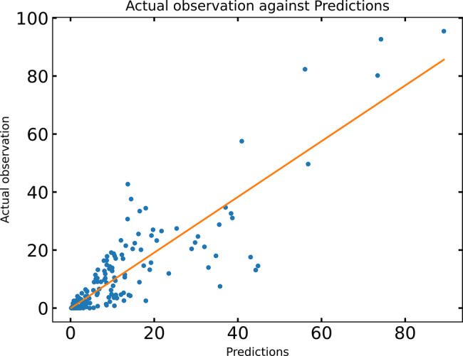
The figure shows from the four constructs in the training data against the prediction of the model. The correlation coefficient R is 0.91
We tested the predictive power of our DNN by confronting it with set of enhancer sequences which the model has not previously seen. The test sequences must be capable of driving expression in D. melanogaster embryos, so that the same TF dataset used for training can be employed to calculate the predicted expression along the A-P axis. In Figure 6, we show the predicted expression of four enhancer sequences, each of which consists of 58 nuclei and hence 58 separate predictions. We chose these enhancers for presentation because they are exceptionally stringent tests in the sense that they involve enhancers with no DNA homology with those used in the training set, either because they are from different genes or distant species. Seventeen additional predictions are given in the Supplementary Material.
Fig. 6.

The figure shows four examples of predictions driven by enhancers not used for training. The location of eve stripes 2 through 7 are shown by vertical dashed lines. The vertical axis shows predicted mRNA concentration; note that the scale for the three graphs to the left of the vertical line differs from the graph on its right. The horizontal axis shows A-P position in % E.L. The enhancers shown are described in the text
We comment in detail on the following predictions. When considering the accuracy of these predictions, it is important to note that the experimental data used for the comparison is in the form of non-quantitative images, which are referred to by specific figure in the citation below. Because the comparison is made to non-quantitative data, it is not possible to assess the quantitative accuracy of the prediction, but only the spatial position. run_str3_7 is the enhancer of the runt gene of D. melanogaster that drives runt stripes 3 and 7, each of which is about 2% E.L. anterior of the corresponding eve stripes. The positions of the stripes are accurate (Klingler et al., 1996; Fig. 3D and K in Klingler et al., 1996). eve_S2E(cyn) and eve_S2E(spp) are respectively the eve stripe 2 enhancers from Sepsis cynipsea and a different but unidentified Sepsis species. eve_s37E(pun) is the stripe 3/7 enhancer from Sepsis punctum. The Sepsis genus is a member of the family Sepsidae, not Drosophilidae, and are so distant from D. melanogaster that there is no sequence homology with the D. melanogaster enhancer longer than a pair of overlapping binding sites (Hare et al., 2008a,b). Nevertheless, all Sepsis enhancers that have been assayed in D. melanogaster embryos drive expression of stripe 2 1–2% E. L. posterior to their native position and stripes 3 and 7 at the native position (Table 2 in Hare et al., 2008b). For eve_S2E(cyn), the predicted stripe 2 is of the correct width and 2% E.L. more posterior than reported. In Sepsidae, stripe 2 enhancer also drives expression of stripe 7. For eve_S2E(cyn), our prediction of stripe 7 expression is completely accurate. For eve_S2E(spp), the predicted stripes are in the correct location, but stripe 2 is significantly wider than observed. For eve_S37E(pun), our prediction for stripe 3 is about 2 nuclei posterior and twice as wide as observed, and for stripe 7, our prediction is completely correct. These predictions demonstrate the generalization capabilities of the DNN implementation of the model. The quality of prediction is comparable to but slightly poorer than the original implementation (in Fig. 4 and Supplementary Fig. S5Kim et al., 2013).
5 Discussion
The work presented here constitutes a strong proof-of-concept for the proposition that DNN can be extremely useful for the construction of precise models of metazoan transcriptional control. Specialized properties of the early Drosophila embryo made it uniquely advantageous for the study of the fundamental properties of metazoan transcription before the onset of genomics. For that reason, it is natural that thermodynamic models of metazoan transcription were developed in Drosophila (Barr and Reinitz, 2017; Barr et al., 2017; Fakhouri et al., 2010; He et al., 2010; Janssens et al., 2006; Kazemian et al., 2010; Kim et al., 2013; Martinez et al., 2014; Reinitz et al., 2003; Samee and Sinha, 2014; Sayal et al., 2016; Segal et al., 2008). As explained in the introduction, we selected what is arguably the most accurate and predictive enhancer level thermodynamic model for reimplementation as a DNN. We have shown that a simpler reimplementation of this model performance almost as well as the original (Kim et al., 2013). The reimplementation is much simpler to code than the original model, amounting to about 600 lines of Keras compared to about 10 000 lines of C++. Implementation in Keras also provides a numerical advantage by permitting the use of backpropagation and stochastic gradient descent for optimization without the need to hand code partial derivatives. As reported above, the use of SGD provides an algorithmic speedup of about 100. Although some issues connected to the wall-clock speedup of the Keras implementation remain, these results suggest that models of this type could be scaled up to much larger datasets. A possible limitation of such generalization is the extensive prior knowledge of details of Drosophila transcription that were used in this study.
There are ample reasons for believing that this lack of prior knowledge can compensated for by increased quantity and quality of computation. In the absence of prior knowledge of the functional roles of TFs, a model very similar to the one we reimplemented here applied to erythropoiesis in mouse (Bertolino et al., 2016) considered all possible combination of TF functional roles and selected the combination which minimized the loss function. The resulting model, while computationally expensive, proved quite predictive (Repele et al., 2019). This shows that extensive prior knowledge is not required.
Until recently, a more serious limitation was the absence of datasets that contained not only information about the sequence but also the concentration of TFs and levels of reporter expression. Such datasets, on a genomic scale, have begun to be available for flies and mammals, including humans (Arnold et al., 2013; Liu et al., 2017; Patwardhan et al., 2009; Smith et al., 2013; Ulirsch et al., 2016). These genomics datasets are much larger than that used in the mouse study (Bertolino et al., 2016). However, the factor of 100 algorithmic speedups, if converted to wall-clock speedup, provides a way forward. The introduction of reinforcement learning techniques may provide further computational efficiency in determining the functional roles of TFs.
With respect to Deep Learning, our model constitutes an example of a fully interpretable DNN that is not merely biologically plausible but biologically validated (Kim et al., 2013). It is our hope that this example will provide insights into the interpretabilities of DNNs in general, a problem that has received wide attention in the community (Boger and Guterman, 1997; Castelvecchi, 2016; Garson, 1991; Li et al., 2015; Maaten and Hinton, 2008; Zeiler and Fergus, 2014).
Funding
This work was supported by award R01OD10936 from the United States National Institutes of Health.
Conflict of Interest: none declared.
Supplementary Material
References
- Abadi M. et al. (2015) TensorFlow: large-scale machine learning on heterogeneous systems. Software available from tensorflow.org (30 September 2019, date last accessed).
- Alipanahi B. et al. (2015) Predicting the sequence specificities of DNA- and RNA-binding proteins by deep learning. Nat. Biotechnol., 33, 831–838. [DOI] [PubMed] [Google Scholar]
- Arnold C.D. et al. (2013) Genome-wide quantitative enhancer activity maps identified by STARR-seq. Science, 339, 1074–1077. [DOI] [PubMed]
- Avsec Ž. et al. (2019) Deep learning at base-resolution reveals motif syntax of the cis-regulatory code. bioRxiv, 737981.
- Barr K.A., Reinitz J. (2017) A sequence level model of an intact locus predicts the location and function of non-additive enhancers. PLoS One, 12, e0180861. [DOI] [PMC free article] [PubMed] [Google Scholar]
- Barr K.A. et al. (2017) Synthetic enhancer design by in silico compensatory evolution reveals flexibility and constraint in cis-regulation. BMC Syst. Biol., 11, 116. [DOI] [PMC free article] [PubMed] [Google Scholar]
- Bertolino E. et al. (2016) The analysis of novel distal Cebpa enhancers and silencers using a transcriptional model reveals the complex regulatory logic of hematopoietic lineage specification. Dev. Biol., 413, 128–144. [DOI] [PMC free article] [PubMed] [Google Scholar]
- Boger Z., Guterman H. (1997) Knowledge extraction from artificial neural network models. In: 1997 IEEE International Conference on Systems, Man, and Cybernetics. Computational Cybernetics and Simulation, Orlando, FL, USA, Vol. 4, pp. 3030–3035. [Google Scholar]
- Burz D.S., Hanes S.D. (2001) Isolation of mutations that disrupt cooperative DNA binding of the Drosophila Bicoid protein. J. Mol. Biol., 305, 219–230. [DOI] [PubMed] [Google Scholar]
- Burz D.S. et al. (1998) Cooperative DNA-binding by Bicoid provides a mechanism for threshold-dependent gene activation in the Drosophila embryo. EMBO J., 17, 5998–6009. [DOI] [PMC free article] [PubMed] [Google Scholar]
- Castelvecchi D. (2016) Can we open the black box of AI? Nat. News, 538, 20–23. [DOI] [PubMed] [Google Scholar]
- Celesti F. et al. (2017) Big data analytics in genomics: the point on deep learning solutions. In: 2017 IEEE Symposium on Computers and Communications (ISCC), pp. 306–309.
- Chollet F. et al. (2015) Keras. https://keras.io, (30 September 2019, date last accessed).
- Cuperus J.T. et al. (2017) Deep learning of the regulatory grammar of yeast 5 untranslated regions from 500,000 random sequences. Genome Res., 27, 2015–2024. [DOI] [PMC free article] [PubMed] [Google Scholar]
- Fakhouri W.D. et al. (2010) Deciphering a transcriptional regulatory code: modeling short-range repression in the Drosophila embryo. Mol. Syst. Biol., 6, 341. [DOI] [PMC free article] [PubMed] [Google Scholar]
- Fujioka M. et al. (1996) Drosophila Paired regulates late even-skipped expression through a composite binding site for the paired domain and the homeodomain. Development, 122, 2697–2707. [DOI] [PubMed] [Google Scholar]
- Garson G.D. (1991) Interpreting neural-network connection weights. AI Expert, 6, 46–51. [Google Scholar]
- Gray S. et al. (1994) Short-range repression permits multiple enhancers to function autonomously within a complex promoter. Genes Dev., 8, 1829–1838. [DOI] [PubMed] [Google Scholar]
- Greenside P. et al. (2018) Discovering epistatic feature interactions from neural network models of regulatory DNA sequences. Bioinformatics, 34, i629–i637. [DOI] [PMC free article] [PubMed] [Google Scholar]
- Hare E.E. et al. (2008. a) A careful look at binding site reorganization in the even-skipped enhancers of Drosophila and sepsids. PLoS Genet., 4, e1000268. [DOI] [PMC free article] [PubMed] [Google Scholar]
- Hare E.E. et al. (2008. b) Sepsid even-skipped enhancers are functionally conserved in Drosopila despite lack of sequence conservation. PLoS Genet., 4, e1000106. [DOI] [PMC free article] [PubMed] [Google Scholar]
- He X. et al. (2010) Thermodynamics-based models of transcriptional regulation by enhancers: the roles of synergistic activation, cooperative binding and short-range repression. PLoS Comput. Biol., 6, e1000935. [DOI] [PMC free article] [PubMed] [Google Scholar]
- Hewitt G.F. et al. (1999) Transcriptional repression by the Drosophila Giant protein: CIS element positioning provides an alternative means of interpreting an effector gradient. Development, 126, 1201–1210. [DOI] [PubMed] [Google Scholar]
- Ilsley G.R. et al. (2013) Cellular resolution models for even skipped regulation in the entire Drosophila embryo. Elife, 2, e00522. [DOI] [PMC free article] [PubMed] [Google Scholar]
- Jaderberg M. et al. (2015) Spatial transformer networks. In: Proceedings of the 28th International Conference on Neural Information Processing Systems, Vol. 2. 2015, MIT Press, Cambridge, MA, USA, pp. 2017–2025.
- Jaeger J. et al. (2004) Dynamic control of positional information in the early Drosophila embryo. Nature, 430, 368–371. [DOI] [PubMed] [Google Scholar]
- Janssens H. et al. (2005) A high-throughput method for quantifying gene expression data from early Drosophila embryos. Dev. Genes Evol., 215, 374–381. [DOI] [PubMed] [Google Scholar]
- Janssens H. et al. (2006) Quantitative and predictive model of transcriptional control of the Drosophila melanogaster even skipped gene. Nat. Genet., 38, 1159–1165. [DOI] [PubMed] [Google Scholar]
- Kazemian M. et al. (2010) Quantitative analysis of the Drosophila segmentation regulatory network using pattern generating potentials. PLoS Biol., 8, e1000456. [DOI] [PMC free article] [PubMed] [Google Scholar]
- Kim A.R. et al. (2013) Rearrangements of 2.5 kilobases of non-coding DNA from the Drosophila even-skipped locus define predictive rules of genomic cis-regulatory logic. PLoS Genet., 9, e1003243. [DOI] [PMC free article] [PubMed] [Google Scholar]
- Kingma D.P., Ba J. (2014) Adam: a method for stochastic optimization. arXiv preprint arXiv : 1412.6980.
- Klingler M. et al. (1996) Disperse versus compact elements for the regulation of runt stripes in Drosophila. Dev. Biol., 177, 73–84. [DOI] [PubMed] [Google Scholar]
- Koh P.W. et al. (2017) Denoising genome-wide histone chip-seq with convolutional neural networks. Bioinformatics, 33, i225–i233. [DOI] [PMC free article] [PubMed] [Google Scholar]
- Koller D. and Friedman N. (2009) Probabilistic Graphical Models: Principles and Techniques. MIT press, Cambridge, MA, USA. [Google Scholar]
- Krizhevsky A. et al. (2012) Imagenet classification with deep convolutional neural networks. In: Proceedings of the 25th International Conference on Neural Information Processing Systems, Vol. 1. Curran Associates, Inc, Red Hook, NY, pp. 1097–1105.
- Lebrecht D. et al. (2005) Bicoid cooperative DNA binding is critical for embryonic patterning in Drosophila. Proc. Natl. Acad. Sci. USA, 102, 13176–13181. [DOI] [PMC free article] [PubMed] [Google Scholar]
- Li Y. et al. (2015) Convergent learning: do different neural networks learn the same representations? In: Proceedings of the 4th International Conference on Learning Representation (ICLR), Commonwealth of Puerto Rico, pp. 196–212.
- Libbrecht M.W., Noble W.S. (2015) Machine learning applications in genetics and genomics. Nat. Rev. Genet., 16, 321–332. [DOI] [PMC free article] [PubMed] [Google Scholar]
- Liu Y. et al. (2017) Functional assessment of human enhancer activities using whole-genome starr-sequencing. Genome Biol., 18, 219. [DOI] [PMC free article] [PubMed] [Google Scholar]
- Ma X. et al. (1996) The Drosophila morphogenetic protein Bicoid binds DNA cooperatively. Development, 112, 1195–1206. [DOI] [PubMed] [Google Scholar]
- Maaten L.V.D., Hinton G. (2008) Visualizing data using t-SNE. J. Machine Learn. Res., 9, 2579–2605. [Google Scholar]
- Manu, et al. (2009) Canalization of gene expression in the Drosophila blastoderm by gap gene cross regulation. PLoS Biol., 7, e1000049. [DOI] [PMC free article] [PubMed] [Google Scholar]
- Martinez C. et al. (2014) Ancestral resurrection of the Drosophila S2E enhancer reveals accessible evolutionary paths through compensatory change. Mol. Biol. Evol., 31, 903–916. [DOI] [PMC free article] [PubMed] [Google Scholar]
- Movva R. et al. (2019) Deciphering regulatory DNA sequences and non-coding genetic variants using neural network models of massively parallel reporter assays. PLoS One, 14, e0218073. [DOI] [PMC free article] [PubMed] [Google Scholar]
- Nair S. et al. (2019) Integrating regulatory DNA sequence and gene expression to predict genome-wide chromatin accessibility across cellular contexts. bioRxiv, 605717. [DOI] [PMC free article] [PubMed]
- Noyes M.B. et al. (2008) A systematic characterization of factors that regulate drosophila segmentation via a bacterial one-hybrid system. Nucleic Acids Res. 36, 2547–2514. [DOI] [PMC free article] [PubMed] [Google Scholar]
- Orgawa N., Biggin M.D. (2012) High-throughput SELEX determination of DNA sequences bound by transcription factors in vitro. Methods Mol. Biol., 786, 51–63. [DOI] [PubMed] [Google Scholar]
- Patwardhan R.P. et al. (2009) High-resolution analysis of DNA regulatory elements by synthetic saturation mutagenesis. Nat. Biotechnol., 27, 1173–1175. [DOI] [PMC free article] [PubMed] [Google Scholar]
- Pouladi F. et al. (2015) Recurrent neural networks for sequential phenotype prediction in genomics. In: 2015 International Conference on Developments of E-Systems Engineering (DeSE), Dubai, pp. 225–230.
- Reinitz J., Sharp D.H. (1995) Mechanism of eve stripe formation. Mechanisms Dev., 49, 133–158. [DOI] [PubMed] [Google Scholar]
- Reinitz J. et al. (2003) Transcriptional control in Drosophila. ComPlexUs, 1, 54–64. [Google Scholar]
- Repele A. et al. (2019) The regulatory control of Cebpa enhancers and silencers in the myeloid and red-blood cell lineages. PLoS One, 14, e0217580. [DOI] [PMC free article] [PubMed] [Google Scholar]
- Roulet E. et al. (2002) High-throughput SELEX SAGE method for quantitative modeling of transcription-factor binding sites. Nat. Biotechnol., 20, 831–835. [DOI] [PubMed] [Google Scholar]
- Rui X. et al. (2007) Inference of genetic regulatory networks with recurrent neural network models using particle swarm optimization. IEEE/ACM Trans. Comput. Biol. Bioinform., 4, 681–692. [DOI] [PubMed] [Google Scholar]
- Samee M.A.H., Sinha S. (2014) Quantitative modeling of a gene’s expression from its intergenic sequence. PLoS Comput. Biol., 10, e1003467–e1003521. [DOI] [PMC free article] [PubMed] [Google Scholar]
- Sayal R. et al. (2016) Quantitative perturbation-based analysis of gene expression predicts enhancer activity in early Drosophila embryo. eLife, 5, e08445. [DOI] [PMC free article] [PubMed] [Google Scholar]
- Segal E. et al. (2008) Predicting expression patterns from regulatory sequence in Drosophila segmentation. Nature, 451, 535–540. [DOI] [PubMed] [Google Scholar]
- Shen J. et al. (2018) Toward deciphering developmental patterning with deep neural network. bioRxiv, 374439.
- Small S. et al. (1992) Regulation of even-skipped stripe 2 in the Drosophila embryo. EMBO J., 11, 4047–4057. [DOI] [PMC free article] [PubMed] [Google Scholar]
- Small S. et al. (1993) Spacing ensures autonomous expression of different stripe enhancers in the even-skipped promoter. Development, 119, 767–772. [PubMed] [Google Scholar]
- Small S. et al. (1996) Regulation of two pair-rule stripes by a single enhancer in the Drosophila embryo. Dev. Biol., 175, 314–324. [DOI] [PubMed] [Google Scholar]
- Smith R.P. et al. (2013) Massively parallel decoding of mammalian regulatory sequences supports a flexible organizational model. Nat. Genet., 45, 1021–1028. [DOI] [PMC free article] [PubMed] [Google Scholar]
- Stanojevic D. et al. (1991) Regulation of a segmentation stripe by overlapping activators and repressors in the Drosophila embryo. Science, 254, 1385–1387. [DOI] [PubMed] [Google Scholar]
- Surkova S. et al. (2008) Characterization of the Drosophila segment determination morphome. Dev. Biol., 313, 844–862. [DOI] [PMC free article] [PubMed] [Google Scholar]
- Ulirsch J.C. et al. (2016) Systematic functional dissection of common genetic variation affecting red blood cell traits. Cell, 165, 1530–1545. [DOI] [PMC free article] [PubMed] [Google Scholar]
- Zeiler M.D., Fergus R. (2014) Visualizing and understanding convolutional networks. In: European Conference on Computer Vision. Springer, . Springer, Berlin , Germany, Cham, pp. 818–833.
Associated Data
This section collects any data citations, data availability statements, or supplementary materials included in this article.