Distance indexing and seed clustering in sequence graphs

Abstract

Motivation

Graph representations of genomes are capable of expressing more genetic variation and can therefore better represent a population than standard linear genomes. However, due to the greater complexity of genome graphs relative to linear genomes, some functions that are trivial on linear genomes become much more difficult in genome graphs. Calculating distance is one such function that is simple in a linear genome but complicated in a graph context. In read mapping algorithms such distance calculations are fundamental to determining if seed alignments could belong to the same mapping.

Results

We have developed an algorithm for quickly calculating the minimum distance between positions on a sequence graph using a minimum distance index. We have also developed an algorithm that uses the distance index to cluster seeds on a graph. We demonstrate that our implementations of these algorithms are efficient and practical to use for a new generation of mapping algorithms based upon genome graphs.

Availability and implementation

Our algorithms have been implemented as part of the vg toolkit and are available at https://github.com/vgteam/vg.

1 Introduction

Conventional reference genomes represent genomes as a string or collection of strings. Accordingly, these so-called ‘linear reference genomes’ can only store one allele at each locus. The resulting lack of diversity introduces a systematic bias that makes samples look more like the reference genome (Zook et al., 2014). This reference bias can be reduced by using pangenomic models, which incorporate the genomic content of populations of individuals (The Computational Pan-Genomics Consortium, 2016). Sequence graphs are a popular representation of pangenomes that can express all of the variation in a pangenome (Paten et al., 2017). Sequence graphs have a more complex structure and the potential to contain more data than linear genomes. This tends to make functions on a sequence graph more computationally challenging than analogous functions on linear genomes.

One such function is computing distance. In a linear genome, the exact distance between two loci can be found by simply subtracting the offset of one locus from the offset of the other. In a graph, calculating distance is much more complicated; there may be multiple paths that connect the two positions and different paths may be relevant for different problems.

Distance is a basic function that is necessary for many functions on genome graphs; in particular, calculating distance is essential for efficient mapping algorithms. In a seed-and-extend paradigm, short seed matches between the query sequence and reference are used to identify small regions for expensive alignment algorithms to align to Garrison et al. (2018), Li (2016), Rakocevic et al. (2019), Rautiainen et al. (2019), Schneeberger et al. (2009) and Vaddadi et al. (2019). Often these regions are identified by clusters of matches. Clustering requires repeated distance calculations between seeds and can be very slow in graphs as large as whole genome graphs. The prohibitive run time of clustering algorithms can make them impractical for mapping and some mapping algorithms omit this step entirely (Rautiainen et al., 2019).

We have developed an algorithm to calculate the exact minimum distance between any two positions in a sequence graph and designed an index to support it. We also developed a clustering algorithm that clusters seeds based on the minimum distance between them. Our algorithms are implemented as part of vg, a variation graph toolkit (Garrison et al., 2018).

2 Background

2.1 Sequence graph structure

A sequence graph is a bidirected graph in which each node is labeled by a sequence of nucleotides. A node X has two sides, $\{x,\overline{x}\}$. For convenience, we will consider x to be the ‘left’ side and $\overline{x}$ to be the ‘right’. This induces a directionality on X, so that we may consider a left-to-right (or x to $\overline{x}$) traversal of X to be forward, and a right-to-left traversal backward. However, we note that the designation of ‘left’ and ‘right’ is arbitrary. They can be swapped without changing the underlying graph formalism. Conceptually, a forward traversal corresponds to the forward strand, and a backward traversal corresponds to the reverse complement strand.

Paths in a bidirected graph must obey restrictions on both nodes and edges. Edges connect two node sides rather than nodes. A path consists of an alternating series of oriented nodes and edges. The path must enter and exit each (non-terminal) node through opposite node sides. In addition, there must exist an edge connecting consecutive nodes in the path, between the node side that is exited and the node side that is entered.

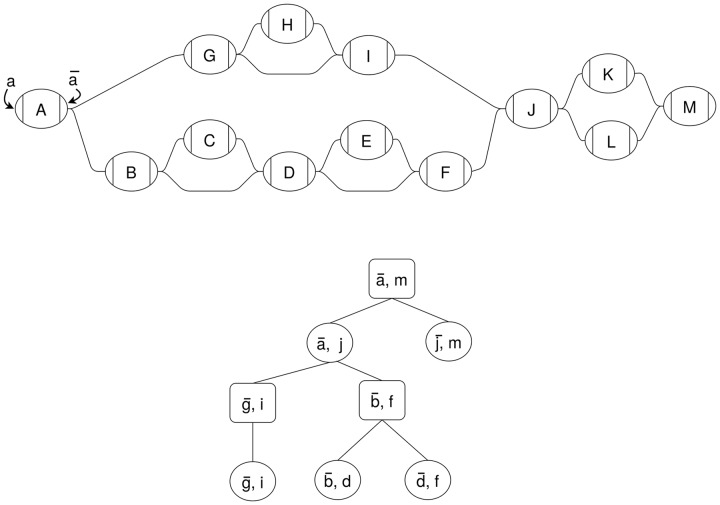
In Figure 1, the graph has an edge between $\overline{a}$ and b. A path including this edge would go from A to B traversing both forward, or from B to A traversing both backward.

Fig. 1.

Example sequence graph (top) and its snarl tree (bottom). Chains in the sequence graph are represented as rectangular nodes in the snarl tree and snarls are represented as elliptical nodes

Some applications use a specific articulation of a sequence graph called a variation graph. A variation graph contains a set of embedded paths through the graph. These paths typically correspond to the primary and alternate scaffolds of a reference genome.

2.2 Snarl decomposition

In previous work, we proposed a decomposition for sequence graphs that describes their common topological features (Paten et al., 2018). A simple variant, such as an indel or SNP, will typically be represented as one or two nodes (corresponding to the different alleles), flanked by two more nodes (corresponding to adjacent conserved sequences. In Figure 1, nodes A, J and M all represent conserved sequences. Nodes K and L represent two alternative sequences that occur between J and M. The subgraph between the two flanking nodes, in this case the subgraph containing nodes J, K, L and M, is called a snarl. Snarls can be seen as a generalization of the variant ‘bubbles’ used in many genome assembly algorithms (Paten et al., 2018).

A snarl is defined by a pair of node sides, (x, y) that delimit a subgraph between them. The nodes X and Y are called the boundary nodes of the snarl. Two node sides define a snarl if they are (i) separable: splitting the boundary nodes into their two node sides disconnects the snarl from the rest of the graph, and (ii) minimal: there is no node A in the snarl such that (x, a) or $(\overline{a},y)$ are separable. In Figure 1, $\overline{g}$ and i define a snarl $(\overline{g},i)$. We will sometimes abuse the terminology and use ‘snarl’ to refer to both the pair of nodes and the subgraph that they separate from the rest of the graph. Thus, we can say that the snarl $(\overline{g},i)$ contains node H and boundary nodes G and I.

In sequence graphs, snarls often occur contiguously with a shared boundary node between them; a sequence of contiguous snarls is called a chain. In Figure 1, the snarls $(\overline{b},d)$ and $(\overline{d},f)$ comprise a chain between $\overline{b}$ and f, which we refer to as $[\overline{b},f]$. A trivial chain is one that contains only one snarl; in Figure 1, snarl $(\overline{g},i)$ is part of a trivial chain, chain $[\overline{g},i]$.

Snarls and chains can be nested within other snarls. This nesting behavior often occurs when the same genomic element is affected by both point and structural variants, in which case the point variant’s snarl nests inside the structural variant’s snarl. A snarl (x, y) contains another snarl (a, b) if all nodes in (a, b) are contained in the subgraph of (x, y). In Figure 1, the snarl $(\overline{a},j)$ contains snarls $(\overline{g},i),\hspace{0.17em}(\overline{b},d)$ and $(\overline{d},f)$. A snarl contains a chain if each of the chain’s snarls are in the subgraph of the containing snarl.

The nesting relationships of snarls and chains in a sequence graph are described by its snarl tree (Fig. 1). Each snarl or chain is represented in the snarl tree as a node. Since every snarl belongs to a (possibly trivial) chain, snarl trees have alternating levels of snarls and chains with a chain at the root of the tree. We also refer to the root as the top-level chain. A snarl is the child of a chain if it is a component of the chain. A chain $[a,b]$ is a child of (x, y) if (x, y) contains $[a,b]$ and there are no snarls contained in (x, y) that also contain $[a,b]$.

All nodes in a sequence graph will be contained by the decomposition of its snarls and chains, described by the snarl tree. In general, the snarl tree can be arbitrarily deep and have very short chains. However, the snarl tree of a typical sequence graph will be shallow and have a long chain as the root. The majority of snarls will be contained in this top-level chain. Small variants can nest within larger structural variants, contributing to the depth of the snarl tree. However, in most parts of the genome, the rate of polymorphism is low enough that two variants are unlikely to overlap each other. As a result, the depth of these nested variants is usually very small, typically <5 in our observations.

Nodes, snarls and chains are all two-ended structures that are connected to the rest of the graph by two node sides. It is sometimes convenient to refer to a topological feature only by this shared property, and to be opaque about which topological feature it actually is. In these cases, we will refer to the node, snarl or chain generically as a ‘structure’. As with nodes of the sequence graph itself, structures are assigned an arbitrary orientation but we will assume that they are oriented left to right and refer to the left and right sides of structures as struct and $\overline{\mathit{struct}}$, respectively. Because of their shared two-ended property, structures can all be treated as single nodes in their parents. The netgraph of a snarl is a view of the snarl where each of its child chains is replaced by a node.

2.3 Prior research

2.3.1 Distance in graphs

Calculating distance in a graph is an extremely well-studied topic. Many graph distance algorithms improve upon classical algorithms, such as Dijkstra’s algorithm (Dijkstra, 1959) and A* (Hart et al., 1968), by storing precomputed data in indexes. These methods index the identities of important edges (Lauther, 2004; Möhring et al., 2005) or distances between selected nodes (Akiba et al., 2013; Dave and Hasan, 2015; Djidjev, 1997; Qiao et al., 2012) then use the indexed information to speed up distance calculations. Index-based algorithms must make a tradeoff between the size of the index and the speed of the distance query.

2.3.2 Distance in sequence graphs

Some sequence graph mapping algorithms use clustering steps based on different estimations of distance (Garrison et al., 2018; Vaddadi et al., 2019). In vg, distance is approximated from the embedded paths. This path-based method estimates the distance between two positions based on a nearby shared path. The algorithm performs a bidirectional Dijkstra search from both positions until it finds at least one path in common from both positions. This path is then used to estimate the distance between them.

Some research has been done on finding solutions for more specific distance queries in sequence graphs. PairG (Jain et al., 2019) is a method for determining the validity of independent mappings of reads in a pair by deciding whether there is a path between the mappings whose distance is within a given range. This algorithm uses an index to determine if there is a valid path between two vertices in a single O(1) lookup. Although this is an efficient solution for this particular problem, it cannot be used to query the exact distance between two nodes. Rather, it returns a boolean value indicating whether two nodes are reachable within a range of distances, which is defined at index construction time.

3 Minimum distance

Our minimum distance algorithm finds the minimum oriented traversal distance between two positions on a sequence graph. A position consists of a node, offset in the sequence, and orientation. The oriented distance must originate from a path that starts traversing the first position in its given orientation and ends at the second position in its given orientation.

Our algorithm uses the snarl decomposition of sequence graphs to guide the calculation. Because structures are connected to the rest of the graph by their boundary nodes, any path from a node inside a structure to any node not in that structure must pass through the structure’s boundary nodes. Similarly, any path between boundary nodes of snarls in a chain must pass through the boundary nodes of every snarl that occurs between them in the chain. Because of this property, we can break up the minimum distance calculation into minimum distances from node and chain boundaries to the boundaries of their parent snarl, from snarl boundaries to their parent chain boundaries, and the distance between sibling structures in their parent structure (Fig. 2). We refer to this property of minimum distance calculation in structures as the split distance property.

Fig. 2.

The minimum distance calculation from a position on C to a position on K can be broken up into the distances from each position to the ends of each of its ancestor structures in the snarl tree. Each colored arrow in the graph represents a distance query from a structure to a boundary node of its parent. The snarl tree node that each query occurs in is outlined with the same color. At the common ancestor of the positions, chain [$\overline{a},m$], the distance is calculated between two of the chain’s children, ($\overline{a},j$) and ($\overline{j},m$)

3.1 Minimum distance index

We designed our minimum distance index to support distance queries between child structures in snarls and between boundary nodes of snarls in chains in constant time. The overall minimum distance index consists of a snarl index for each snarl and a chain index for each chain in the graph.

3.1.1 Snarl index

For each snarl, the index stores the minimum distances between every pair of node sides of child structures contained in the snarl, including the boundary nodes. A distance query within a snarl is a simple constant time lookup of the distance.

3.1.2 Chain index

For each chain, the index stores three arrays, each with one entry for each boundary node of the snarls in the chain. The first, a prefix sum array, contains the minimum distance from the start of the chain to the left side of each of the boundary nodes of the snarls that comprise the chain. This array can be used to find the distance between two of these snarls’ boundary nodes along the chain. Distances from a left-to-right traversal of the chain can be computed directly from the prefix sum array, whereas distances from a right-to-left traversal also require the length of the boundary nodes. Since paths can reverse direction in the chain (Fig. 3a), the index also stores each boundary node’s ‘loop distance’. The loop distance is the minimum distance to leave a boundary node, change direction in the chain and return to the same node side traversing in the opposite direction. These loop distances are stored in final two arrays, one for each direction. In Figure 3a, the forward loop distance for node C is two times the length of E: the distance to leave $\overline{c}$ traversing forward and return to $\overline{c}$ traversing backward by taking the bold looping edge on $\overline{e}$. These three arrays are sufficient to find the minimum distance between any two node sides in the chain in constant time (Fig. 3).

Fig. 3.

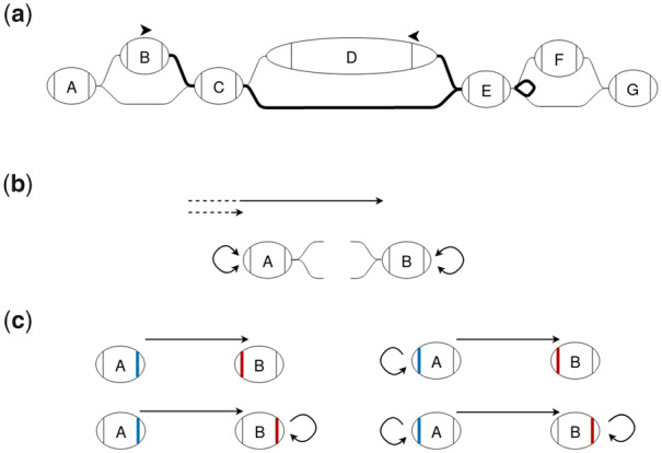
(a) The shortest path between two nodes in a chain can sometimes reverse direction in the chain. The edges on the shortest path between the positions on B and D are bolded. (b) A and B are boundary nodes of snarls in a chain. Distances stored in the chain index are shown in black. For each boundary node in the chain, the chain index stores the minimum distance from the start of the chain to the left side of that node as well as the loop distances for a forward and backward traversal. These loop distances are the minimum distance to leave a node, reverse direction in the chain and return to the same node side. (c) There are four possible minimum-distance paths between two nodes, connecting either node side of the two nodes. The lengths of these paths can be found using the distances stored in the chain index and the lengths of the nodes

Chains that are not top-level chains cannot form a closed cycle so any path that traverses a chain’s boundary node going out of the chain must leave the chain. Therefore, any connectivity between the boundaries of the chain will be captured by the snarl index of the chain’s parent. The top-level chain may form a closed cycle where the start and end boundary nodes are the same node (Fig. 4). In this case, the shortest path may remain within the chain, but it may also leave the chain and re-enter it from the other side. In Figure 4, the minimum distance from $\overline{a}$ to d could be $d(\overline{a},\overline{d})+d(d,d)$ or $d(\overline{a},\overline{a})+d(a,d)$.

Fig. 4.

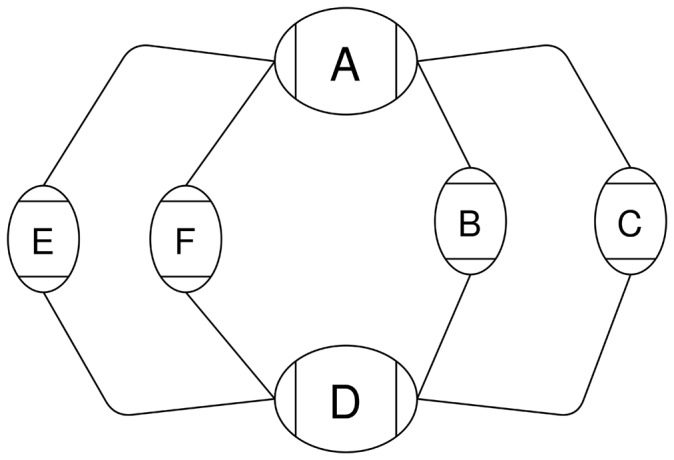
A cyclic chain containing two snarls, $(\overline{a},\overline{d})$ and (d, a)

3.1.3 Index construction

The minimum distance index is constructed in a post-order traversal of the snarl tree. For each snarl, the construction algorithm does a Dijkstra traversal starting from each child structure, using the child’s index to find the distance to traverse child snarls or chains. For each chain, the construction algorithm traverses through each snarl in the chain and uses the snarl’s index to find each of the relevant distances for the chain index.

3.1.4 Index size

Naively, a minimum distance index could store the minimum distance between every node in the graph. A distance calculation would be a constant time lookup but the index size would be quadratic in the number of nodes in the graph. For each snarl in the graph, our index stores the distance between every pair of structures in the net graph. For each chain, it stores three arrays, each the length of the chain. In a graph with a set of snarls S and chains C, our index will take $O(\sum _S{n}_s^2+\sum _C{n}_c)$ space where n_s is the number of structures in the netgraph of snarl s and n_c is the number of snarls in chain c.

3.2 Minimum distance algorithm

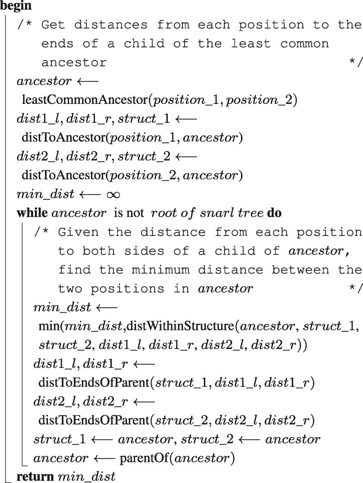
The first step of our minimum distance algorithm (Algorithm 2) is to find the least common ancestor structure in the snarl tree that contains both positions. We do this by traversing up the snarl tree from each position and finding the first common structure. This traversal is O(d) where d is the depth of the snarl tree.

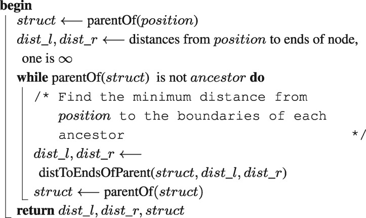
Next, the algorithm finds the distance from each position to the ends of the child of the least common ancestor (Algorithm 1). Starting at a position on a node, we find the distances to the ends of the node. If both positions are oriented forward, then we find the distance to the right side of the fist node and the left side of the second, and we record the distances to the opposite sides as infinite. In the case where a position is oriented backward, we find the distance to the opposite side. The algorithm then traverses up the snarl tree to the least common ancestor and at each structure, finds the minimum distances to the ends of the structure. Because of the split distance property, this distance can be found by adding the distances to the ends of the child, found in the previous step in the traversal, to the distances from the child to the boundary nodes of the structure, found using the minimum distance index (Fig. 5). Since this requires only four constant-time queries to the minimum distance index, each step in the traversal is constant time and the overall traversal is O(d).

Fig. 5.

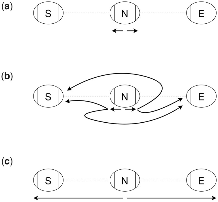
The distToEndsOfParent calculation described in Table 1. (a) S and E are the boundary nodes of a structure that contains a child structure N. The minimum distances from some object in N to the ends of N shown as black arrows. (b) The minimum distances from each end of N to $\overline{s}$ and e are found using the minimum distance index. (c) By adding the appropriate distances and taking the minimums, we can get the minimum distances to s and $\overline{e}$

Table 1.

Primitive functions for the minimum distance algorithm

Function	Description	Complexity
distToEndsOfParent (struct, dist_left, dist_right)	Given the distances from a position in a structure struct to the ends of struct, find the distance to the ends of the parent (Fig. 5)	O(1) using the distance index
distWithinStructure (struct, child_1, child_2, dist1_l, dist_2_l, dist2_r)	Given two children of a structure and distances from positions to the boundaries of the children, find the minimum distance between the positions in struct	O(1) using the distance index

At this point in the algorithm, we know the minimum distance from each position to its ancestor structure that is a child of the common ancestor. By composing these distances with the distances between the two structures, the algorithm finds possible distances between the two positions in the common ancestor structure. The algorithm continues to traverse the snarl tree up to the root and finds a minimum distance between the positions at each structure, checking for paths that leave the lowest common ancestor. This traversal is also O(d). The minimum distance algorithm is done in three O(d) traversals of the snarl tree, so the algorithm is O(d). In variation graphs for moderately large genomes without extreme levels of polymorphism, snarl trees are very shallow. In these graphs, the algorithm is expected to be O(1). However, for variation graphs of small, highly polymorphic genomes, the run time may grow with increasing amounts of population variation. Complex sequence graphs derived from assembly graphs also may demonstrate slower run time behavior.

Algorithm 1: distToAncestor(position, ancestor): given a position and ancestor structure, return the minimum distance from the position to both sides of a child of the ancestor and the child

Algorithm 2: minDistance($\mathit{position}\_1,\mathit{position}\_2$): return the minimum distance from $\mathit{position}\_1$ to $\mathit{position}\_2,\hspace{0.17em}\infty$ if no path between them exists

4 Clustering

Seed-and-extend algorithms sometimes cluster seed alignments by their location in the graph to find which might belong to the same mapping. Using our minimum distance index, we developed an algorithm to cluster positions based on the minimum distance between them in the graph.

4.1 Problem

We will cluster seeds by partitioning them based on the minimum distance between their positions in a sequence graph. To define a cluster, we consider a graph where each seed is a node and two seeds are connected if the minimum distance between their positions is less than a given distance limit. In this graph, each connected component is a cluster.

4.2 Algorithm

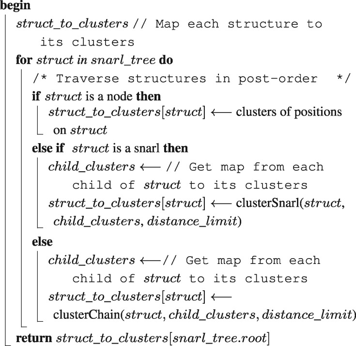
Our clustering algorithm starts with each position in a separate cluster then progressively agglomerates the clusters (Fig. 6). The algorithm proceeds in a post-order traversal of the snarl tree and, at each structure, produces clusters of all positions contained in that structure (Algorithm 5). After iterating over a structure, clusters are also annotated with two ‘boundary distances’: the shortest distance from any of its positions to the boundary nodes of the structure. At every iteration, each cluster can be unambiguously identified with a structure and so the boundary distances are always measured to the structure the cluster is on.

Fig. 6.

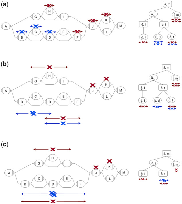
Clustering of positions (Xs) is done by traversing up the snarl tree and progressively agglomerating clusters. Positions are colored by the final clusters. (a) Each position starts out in a separate cluster on a node. Each cluster is annotated with its boundary distances: the minimum distances from any of its positions to the ends of the structure it is on. (b) For each snarl on the lowest level of the snarl tree, the clusters on the snarl’s children are agglomerated into new clusters on the snarl. The boundary distances are extended to the ends of the snarl. (c) For each chain on the next level of the snarl tree, the clusters on the chain’s snarls are agglomerated and the boundary distances are updated to reach the ends of the chain. This process is repeated on each level of the snarl tree up to the root

The method of agglomerating clusters and computing boundary distances vary according to the type of structure. For nodes, the algorithm creates a sorted array of the positions contained in it and splits the array into separate clusters when the distance between successive positions is large enough. For each new cluster, the boundary distances are computed from the positions’ offsets.

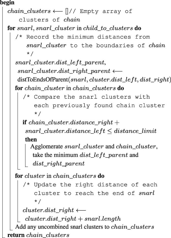
For structures that are snarls or chains, clusters are created from the clusters on their children (Algorithms 3 and 4). Clusters associated with child structures are compared and if the distance between any pair of their positions is smaller than the distance limit, they are combined. Within a structure, distances to clusters that are associated with child structures can be calculated using the split distance property as in the minimum distance algorithm. According to this property, the minimum distance can be split into the cluster’s boundary distance and the distance to one of the boundary nodes, which is found using the index. For snarls, all pairs of clusters are compared with each other. For chains, clusters are combined in the order they occur in the chain, so each cluster is compared with agglomerated clusters that preceded it in the chain. Finally, for each of the resulting clusters, we compute the boundary distances for the current structure, once again using the boundary distances of the children and the index.

In the worst case, every position would belong to a separate cluster and at every level of the snarl tree, every cluster would be compared with every other cluster. This would be $O(d{n}^2)$ where d is the depth of the snarl tree and n is the number of seeds, so in the worst case our clustering algorithm is no better than the naive algorithm of comparing every pair of positions with our minimum distance algorithm. In practice, however, seeds that came from the same alignment would be near each other on the graph and form clusters together, significantly reducing the number of distance comparisons that would be made (see Section 5).

Algorithm 3: clusterSnarl(snarl, child_to_clusters, distance_limit): given a snarl and map from children of the snarl to their clusters, get clusters of the snarl

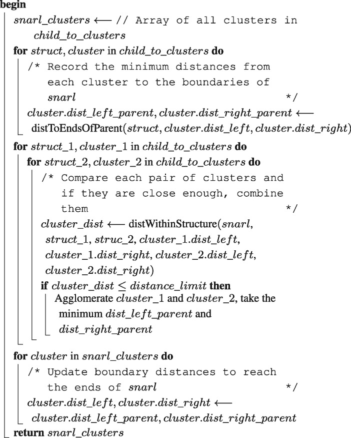
Algorithm 4: clusterChain(chain, child_to_clusters, distance_ limit): given a chain and a map from each snarl in the chain to its clusters, get clusters of the chain

5 Methods and results

Our algorithms are implemented as part of the vg toolkit. We conducted experiments on two different graphs: a human genome variation graph and a graph with simulated structural variants. The human genome variation graph was constructed from GRCh37 and the variants from the 1000 Genomes Project. The structural variant graph was simulated with 10 bp to 1 kb insertions and deletions every 500 bp.

The human genome variation graph had 306 009 792 nodes, 396 177 818 edges and 3 180 963 531 bp of sequence. The snarl tree for this graph had a maximum depth of 3 snarls with 139 418 023 snarls and 11 941 chains. The minimum distance index for the graph was 12.2 GB on disk and 17.7 GB in memory.

To assess the run time of our minimum distance algorithm, we calculated distances between positions on the whole genome graph and compared the run time of our algorithm with vg’s path-based algorithm and Dijkstra’s algorithm (Fig. 7). We chose random pairs of positions in two ways. The first method sampled positions uniformly at random throughout the graph. The second method first followed a random walk of 148 bp through the graph and then sampled two positions uniformly at random from this random walk. This approach was intended to approximate the case of seeds from a next-generation sequencing read. On average, our minimum distance algorithm is the fastest of the three algorithms for both sets of positions. In addition, all three algorithms’ performance degraded when the positions could be sampled arbitrarily far apart in the graph, but our minimum distance algorithm’s performance degraded the least.

Fig. 7.

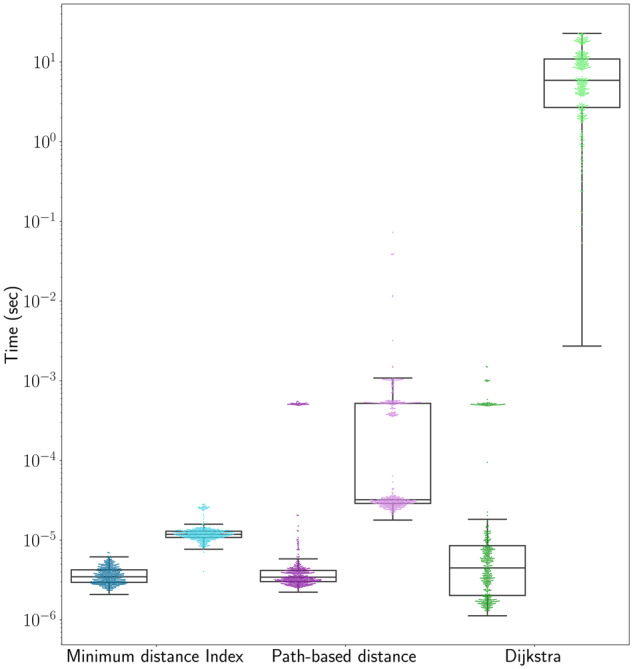
Run times for distance algorithms. Random pairs of positions were chosen from either within a read-length random walk (dark colors) or randomly from the graph (light colors)

Our new minimum distance algorithm shows a distinct gain in performance over the other methods, however, the algorithm must trade off speed with the memory consumed by the index. A hybrid approach could be imagined where the index is used to compute the distance up structures in the common ancestor, then Dijkstra’s algorithm could be used to connect the structures. The runtime of such a hybrid algorithm is in the worst case the same as Dijkstra’s algorithm. Using this approach, the distance index would only need to store the distance from each node in a snarl to the boundary nodes of the snarl, rather than the distance between every pair of nodes, reducing the memory requirement of the index.

In the context of read mapping, we are often only interested in the exact distance when the minimum distance is small, but when the minimum distance is large enough the exact distance is not necessary. In this scenario, the algorithm could be accelerated by stopping early when it is apparent that the minimum distance will be too large.

We used the structural variant graph to assess whether the minimum distance is a useful measure of distance for read mapping. We compared our minimum distance algorithm with the path-based approximation, which estimates distances based on linear paths corresponding to scaffolds of a reference genome. To do so, we again used read-length random walks to select pairs of positions. Further, we filtered random walks down to those that overlapped a structural variant breakpoint. We then calculated the distances between pairs of positions using our minimum distance algorithm and the path-based approximation and compared these distances with the actual distances in the random walk, which we take as an approximation of the true distance on a sequencing read. Overall, the minimum distance was a much better estimate of distance along the random walk than the path-based distance approximation (Fig. 8).

Fig. 8.

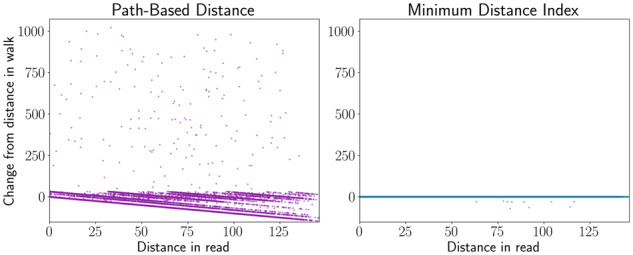
Distance calculations on a graph with simulated structural variants. Read-length random walks were simulated near the junctions of structural variants. The distance between two random positions along each walk was calculated using the path-based method and our minimum distance algorithm and compared with the actual distance in the walk

For our clustering algorithm, we wanted to estimate the run time of the algorithm in the context of read mapping. We simulated 148 bp reads from AshkenazimTrio HG002_NA24385_son from the Genome in a Bottle Consortium (Zook et al., 2016). For each read, we sampled 15-mer matches from the read and found their positions in the human genome variation graph using a k-mer lookup table. We then apply the clustering algorithm to the positions of these k-mers. The regression line of the log−log plot of run times suggests the run time of our algorithm is linear in the number of positions in practice, despite the quadratic worst-case bound (Fig. 9).

Fig. 9.

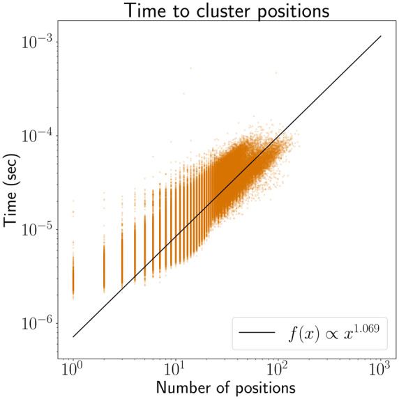
Run time growth of our clustering algorithm. The regression line suggests that the run time of our algorithm is approximately linear in the number of positions in practice

6 Conclusion

Pangenomes have the potential to eliminate reference bias and grow the inclusiveness of reference structures used in genomics, but substantial algorithmic challenges remain in adapting existing paradigms to use them. We have developed a simple and elegant minimum distance algorithm with run time that is linear in the depth of the snarl tree. In practice, the algorithm exploits the observation that real-world genome graphs have an excess of small, local variations and relatively fewer variations that connect disparate parts of the graph. The result is that real genome graphs have a shallow snarl tree, making the calculations fast and effectively constant time in practice; indeed, we observe the algorithm is substantially faster than other distance algorithms on queries of arbitrary distance. The minimum distance we return is an exact distance, unlike the previous heuristic implementation of distance in vg, resulting in much more reasonable estimates of distance around the breakpoints of structural variants. Our minimum distance algorithm will also work with any sequence graph, whereas the preexisting vg distance algorithm required pre-specified paths. Here we developed a clustering algorithm for clustering positions on the graph based on the minimum distances between them. Clustering is a major component of many mapping algorithms and calculating distance is a bottleneck of clustering in genome graphs. Our new clustering algorithm runs in linear time relative to the number of seeds, whereas many existing algorithms, including the current vg mapper’s path-based algorithm, are (at least) quadratic due to pairwise distance calculations between seeds. We believe this is an important step in generalizing efficient mapping algorithms to work with genome graphs; we are now developing fast mapping algorithms that use this clustering algorithm.

Algorithm 5: cluster(snarl_tree, positions, distance_limit): Cluster positions based on the distance limit

Funding

This work was supported, in part, by the National Institutes of Health [award numbers: 5U54HG007990, 5T32HG008345-04, 1U01HL137183, R01HG010053, U01HL137183 and 2U41HG007234].

Conflict of Interest: none declared.

References

- Akiba T. et al. (2013) Fast exact shortest-path distance queries on large networks by pruned landmark labeling. In Proceedings of the 2013 International Conference on Management of Data - SIGMOD’13, ACM Press, New York, NY, USA, p. 349.
- Dave V.S., Hasan M.A. (2015) TopCom: index for shortest distance query in directed graph In Q Chen. et al. (eds) Database and Expert Systems Applications, Lecture Notes in Computer Science, Springer International Publishing, Cham, pp. 471–480. [Google Scholar]
- Dijkstra E.W. (1959) A note on two problems in connexion with graphs. Numer. Math., 1, 269–271. [Google Scholar]
- Djidjev H.N. (1997) Efficient algorithms for shortest path queries in planar digraphs In: G. Gooset al. (eds) Graph-Theoretic Concepts in Computer Science. Vol. 1197, Springer, Berlin, Heidelberg, pp. 151–165. [Google Scholar]
- Garrison E. et al. (2018) Variation graph toolkit improves read mapping by representing genetic variation in the reference. Nat. Biotechnol., 36, 875–879. [DOI] [PMC free article] [PubMed] [Google Scholar]
- Hart P.E. et al. (1968) A formal basis for the heuristic determination of minimum cost paths. IEEE Trans. Syst. Sci. Cybernetics, 4, 100–107. [Google Scholar]
- Jain C. et al. (2019) Validating paired-end read alignments in sequence graphs. In: Huber, KT. et al (eds) 19th International Workshop on Algorithms in Bioinformatics (WABI 2019)., Vol. 142, Leibniz International Proceedings in Informatics (LIPIcs), Dagstuhl, Germany: Schloss Dagstuhl -- Leibniz-Zentrum fuer Informatik, pp.17:1--17:13.
- Lauther U. (2004) An extremely fast, exact algorithm for finding shortest paths in static networks with geographical background In: Raubal M.et al. (eds) Geoinformation und Mobilität - von der Forschung zur praktischen Anwendung, IfGI prints, Vol 22, Institut für Geoinformatik, Münster, pp.219–230. [Google Scholar]
- Li H. (2016) Minimap and miniasm: fast mapping and de novo assembly for noisy long sequences. Bioinformatics, 32, 2103–2110. [DOI] [PMC free article] [PubMed] [Google Scholar]
- Möhring R.H. et al. (2005) Partitioning graphs to speed up Dijkstra’s algorithm In: Hutchison D.et al. (eds) Experimental and Efficient Algorithms. Vol. 3503, Springer, Berlin, Heidelberg, pp. 189–202. [Google Scholar]
- Paten B. et al. (2017) Genome graphs and the evolution of genome inference. Genome Res., 27, 665–676. [DOI] [PMC free article] [PubMed] [Google Scholar]
- Paten B. et al. (2018) Superbubbles, ultrabubbles, and cacti. J. Comput. Biol., 25, 649–663. [DOI] [PMC free article] [PubMed] [Google Scholar]
- Qiao M. et al. (2012) Approximate shortest distance computing: a query-dependent local landmark scheme. In: 2012 IEEE 28th International Conference on Data Engineering, IEEE, Washington, D.C., USA, 1-5 April 2012, pp. 462–473, ISSN:2375-026X,1063-6382. [Google Scholar]
- Rakocevic G. et al. (2019) Fast and accurate genomic analyses using genome graphs. Nat. Genet., 51, 354–362. [DOI] [PubMed] [Google Scholar]
- Rautiainen M. et al. (2019) Bit-parallel sequence-to-graph alignment. Bioinformatics, 35, 3599–3607. [DOI] [PMC free article] [PubMed] [Google Scholar]
- Schneeberger K. et al. (2009) Simultaneous alignment of short reads against multiple genomes. Genome Biol., 10, R98. [DOI] [PMC free article] [PubMed] [Google Scholar]
- The Computational Pan-Genomics Consortium. (2016) Computational pan-genomics: status, promises and challenges. Brief. Bioinformatics,19, 118–135. [DOI] [PMC free article] [PubMed] [Google Scholar]
- Vaddadi K. et al. (2019) Read Mapping on Genome Variation Graphs In: Huber, KT. et al (eds) 19th International Workshop on Algorithms in Bioinformatics (WABI 2019), Vol. 142, Leibniz International Proceedings in Informatics (LIPIcs), Dagstuhl, Germany: Schloss Dagstuhl -- Leibniz-Zentrum fuer Informatik, pp.7:1--7:17.
- Zook J.M. et al. (2014) Integrating human sequence data sets provides a resource of benchmark SNP and indel genotype calls. Nat. Biotechnol., 32, 246–251. [DOI] [PubMed] [Google Scholar]
- Zook J.M. et al. (2016) Extensive sequencing of seven human genomes to characterize benchmark reference materials. Scientific Data, 3, 160025. [DOI] [PMC free article] [PubMed] [Google Scholar]