GLIDE: combining local methods and diffusion state embeddings to predict missing interactions in biological networks

Abstract

Motivation

One of the core problems in the analysis of biological networks is the link prediction problem. In particular, existing interactions networks are noisy and incomplete snapshots of the true network, with many true links missing because those interactions have not yet been experimentally observed. Methods to predict missing links have been more extensively studied for social than for biological networks; it was recently argued that there is some special structure in protein–protein interaction (PPI) network data that might mean that alternate methods may outperform the best methods for social networks. Based on a generalization of the diffusion state distance, we design a new embedding-based link prediction method called global and local integrated diffusion embedding (GLIDE). GLIDE is designed to effectively capture global network structure, combined with alternative network type-specific customized measures that capture local network structure. We test GLIDE on a collection of three recently curated human biological networks derived from the 2016 DREAM disease module identification challenge as well as a classical version of the yeast PPI network in rigorous cross validation experiments.

Results

We indeed find that different local network structure is dominant in different types of biological networks. We find that the simple local network measures are dominant in the highly connected network core between hub genes, but that GLIDE’s global embedding measure adds value in the rest of the network. For example, we make GLIDE-based link predictions from genes known to be involved in Crohn’s disease, to genes that are not known to have an association, and make some new predictions, finding support in other network data and the literature.

Availability and implementation

GLIDE can be downloaded at https://bitbucket.org/kap_devkota/glide.

Supplementary information

Supplementary data are available at Bioinformatics online.

1 Introduction

All current protein–protein interaction (PPI) or other protein–protein association networks derived from heterogeneous types of biological data are in fact noisy and incomplete snapshots of the true network, where it is assumed that false positives (edges placed in the network that in fact, should not exist) are not as large a problem as false negatives, i.e. the true networks contain many true links that are missing because those interactions have not yet been experimentally observed; see estimations in Menche et al. (2015) and Venkatesan et al. (2009) for PPI networks derived from physical interaction data. Thus, link prediction is a core problem of interest in these networks. Methods to predict missing links have been more studied in the social network analysis community (see Al Hasan and Zaki, 2011; Li et al., 2018b; Wang et al., 2015, for surveys) than for biological networks, but there is indeed some past work that proposed and tested new link prediction methods on PPI networks (Cannistraci et al., 2013; Hulovatyy et al., 2014; Kuchaiev et al., 2009; Lei and Ruan, 2013), including a recent paper of Kovács et al. (2019).

In social networks, a lot of the network structure is dominated by ‘triadic closure’: the principle that friends of my friends are more likely to be friends of each other (completing the triangle). However, recently Kovács et al. (2019) argued successfully that for some types of biological networks, a different structure was more likely to be at play. Namely, that if two nodes had a large number of common neighbors, rather than predicting the nodes be neighbors, we should instead predict that the rest of the neighbors of each also interacted with the original node. This models two proteins interacting with the same set of receptors (Fig. 1). Note that, this alternative local measure can also predict links between nodes of shortest-path distance three in the graph, whereas triadic closure solely predicts connections between nodes that are shortest-path distance two apart.

Fig. 1.

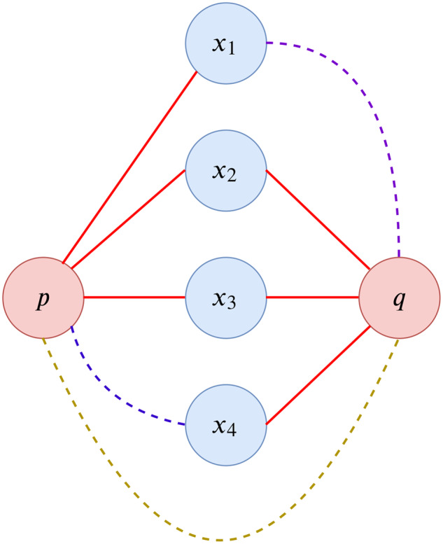
Solid lines represent actual network edges. In triadic closure, we would predict the dotted yellow edge (p, q) with high confidence, because p and q have many common neighbors. In L3, we would first predict the dotted purple edges $(p,x_4)$ and $(q,x_1)$

We were interested in looking at a heterogeneous collection of biological networks, to determine when each of these principles is dominant. In particular, we consider the first three of the networks that were used in the 2016 DREAM disease module challenge (Choobdar et al., 2019), and see if a common neighbors statistic (that rewards triadic closure) or the L3 statistic is a better predictor of missing links. However, both these measures are good predictors only when two nodes have common neighbors. Thus, we propose a novel link prediction method called global and local integrated diffusion embedding (GLIDE). GLIDE predicts either based on common neighbors or L3 when there are many common neighbors, and otherwise uses a new embedding-based distance method based on a generalization of the diffusion state distance (DSD) (Cao et al., 2013, 2014). We show that GLIDE outperforms both the state-of-the-art node2vec (Grover and Leskovec, 2016), and at least matches and often outperforms the baseline L3 and common neighbors statistics for link prediction in rigorous cross-validation experiments.

We look in depth at what interesting links GLIDE predicts in the sparsest of the networks, we consider, DREAM3. We discover and predict some new genes involved in the disease pathology of Crohn’s disease, as an example use of the method.

1.1 The link prediction problem

The link prediction problem is studied in two settings. In one setting, the missing links are assumed to be unobserved interactions in a network. The simplest model assumes that each link has an equal and independent probability of being missing from the observed network, though in practice, the set of observed observations may be biased by how well studied its endpoints are, or the ease of detecting interactions may not be node independent even in the case that experiments test for possible missing links at random. Still, the performance of link-prediction algorithms can be benchmarked in this setting by taking a PPI network, randomly removing 5, 10% or some other fraction of the known links, using the remaining network as the training data, and seeing how well the algorithm predicts the missing removed links.

The second setting involves looking at an older snapshot of the network, and trying to predict the set of new links that have been added over time to reach the present-day instance of the network. For example we can take the BioGRID Saccharomyces cerevisiae database in 2014 (Cao et al., 2014), and attempt to predict new links that are included in the BioGRID database of 2019. This setting better models the problem of predicting the edges that will show up in future versions of existing databases, both as the new edges will be biased by how well studied the proteins are, and because new experiments often test a smaller set of target proteins against a large panel of potential interacting partners, meaning that the pattern of newly added interactions will be different than a completely random sample of the missing edges.

This second scenario can be modeled as follows. Suppose we have a graph $G=(V,E)$ in which each edge $e=(u,v)\in E$ represents an interaction between u and v that took place at a particular time t₀. If we record those interactions in a different time $t_1>t_0$, obtaining some new set of interactions and add them to create a new graph $G\prime =(V,E\prime )$, where $E\subset E\prime$, then the link prediction problem would be described in the following way: design an algorithm that uses the original graph G as the training set to predict the new interactions in $G\prime$.

In what follows, we test our methods in the first setting on three human protein–protein association networks that were released as part of the 2016 DREAM disease module challenge (Choobdar et al., 2019) (termed DREAM1, DREAM2 and DREAM3 in the challenge). DREAM2, derived from InWeb version 3 (Li et al., 2017), is a classical PPI network, which aggregates physical PPI links from primary databases and the literature. DREAM1 is derived from STRING version 10.0 (Szklarczyk et al., 2015). STRING contains not only protein–protein physical interactions, but also co-expression links, and other types of experimentally derived interactions. Note that, associations derived from text-mining were removed from STRING when DREAM1 was constructed. DREAM3 is the OmniPath signaling network, which integrates literature-curated human signaling pathways from 27 different sources (Türei et al., 2016). For our purposes, we treat it in this work as an undirected network. [We note that the DREAM challenge also included networks 4–6 described and available from (Li et al., 2018a) which were constructed from very different types of association data, and which we did not use.] For each network, we construct five different instances of reduced networks with deleted links: we protect a random spanning tree so that the network remains connected, and then remove 10% of the links in DREAM1-3. All our reported performance statistics are based on the mean and standard deviation of prediction performance over the five different experiments (removing a different random 10% of the edges) for each of the networks.

In the second setting, we take two snapshots of the S. cerevisiae PPI network on BioGRID, with confidences assigned as in the paper of Cao et al. (2014). The older version of BioGRID used in Cao et al. (2014) and downloadable from http://dsd.cs.tufts.edu/capdsd/ is used as the first snapshot, and the task is to try to predict the new links from the most recent version of the yeast BioGRID network.

The graph properties, number of vertices, edges, average degree, diameter and clustering coefficient of the largest connected component of DREAM1-3 and BioGRID networks are shown in Table 1.

Table 1.

Graph properties of the largest connected components of the human DREAM 1–3 networks and the yeast BioGRID network

Graph	# Nodes	# Edges	Average degree	Diameter	Clustering coefficient
DREAM1	17 388	2 232 398	11.63	7	0.34
DREAM2	12 325	397 254	11.63	9	0.34
DREAM3	5009	18 270	11.45	12	0.20
BioGRID (2014)	4996	76 010	11.45	5	0.31
BioGRID (2017)	4996	107 769	11.45	5	0.38

Note: Note that in addition, we restricted the connected components of BioGRID (2014) and BioGRID (2017) networks to have the same set of vertices. We also removed edges in BioGRID (2014) that were not present in BioGRID (2017).

For each network, in both settings we look at two different types of rankings for evaluation. The first ranking globally ranks all possible nonedges as missing links, and we can compute precision–recall and receiver operating characteristic (ROC) statistics. The second is a ‘node-based’ ranking, where we fix a particular node v, and require a ranking of all possible nonedges that have v as an endpoint (i.e. predict links from node v). We measure the performance in a node-based ranking setting by randomly selecting 1000 nodes that have at least 1 missing link in the test network, and computing the average precision–recall and ROC statistics over all these nodes. The first setting will have the initial portion of the link rankings dominated by highly connected hub genes when the network has a densely connected core. The second setting can focus also on less dense network regions by singling out connections to particular nodes, many of which are not hubs.

2 Previous work

All the methods for link prediction in this article, both our new method and previous methods, can be described by a pairwise score that is assigned to every pair of vertices that does not have an observed edge between them, and then the possible links are rank ordered by score. Good methods put the true missing links towards the top of the list. A parameter can set a cutoff on the ranked list, and predict links for every potential edge above the cutoff and no link for every potential edge below, resolving the ranked list into a binary classification of predict link/no link. Then ROC and precision–recall curves can be computed to compare the qualities of competing ranking methods. Specifically, the area under the ROC and precision–recall curves—denoted AUROC and AUPRC, respectively—of different methods can be compared. We note that because of the extreme class imbalance (almost every pair of nodes represents a nonedge; any classifier which always says ‘no link’ has a terrific AUROC), precision–recall and AUPRC are more informative measures than ROC and AUROC; we still report ROC and AUROC in Supplementary Material, because as a comparative measure for competing methods, the curves are informative. However, the extreme class imbalance means that in absolute terms, AUROC values will seem very high and AUPRC values will seem very low for this problem.

Liben-Nowell and Kleinberg (2007) tested a large number of basic ranking measures on a subset of the co-authorship network for papers submitted to the Physics section of the arXiv preprint server. The authors trained on the network of co-authorship links from papers written between 1994 and 1996, and then tried to predict new co-author pairs on papers written between 1997 and 1999. The measures they tested included weighted and unweighted versions of common neighbors, Jaccard coefficient and a neighborhood-based score (Adamic and Adar, 2003). When we compared the AUROC of these measures on DREAM1–3, the common neighbors (weighted) metric did the best (see Supplementary Table S2). Thus, we included the common neighbors (weighted) measure in our experiments below.

There is a recent evidence that the best embedding methods perform better than these baseline measures tested by Liben-Nowell and Kleinberg (2007), at least in the social network domain. These methods embed the graph into a Euclidean space, and the potential link between a pair of nodes is ranked based on the inverse of their distance in the Euclidean space. One popular and highly successful embedding method is node2vec (Grover and Leskovec, 2016). Most embedding methods studied to date were not designed for biological networks; an excellent recent survey of embedding methods applied to biological network problems appears in Nelson et al. (2019).

Kovács et al. (2019) argued that many of the measures studied by Liben-Nowell and Kleinberg (2007) should not perform as well on PPI networks as they do on social networks, because triadic closure (the tendency of paths of length two to indicate missing triangles) did not hold as often in the PPI network. Instead, they designed a new measure they called L3, more similar to common neighbors than the other Liben-Nowell and Kleinberg (2007) measures, to capture that proteins with many overlapping interacting partners should be predicted to interact with other members of the partner set, to a greater extent than they should be predicted to interact with each other. However, they tested their new measure only against the basic measures of Liben-Nowell and Kleinberg (2007); they did not test against any of the embedding measures.

In this article, we introduce a novel embedding measure based on a normalized diffusion state embedding. Our ranking method function fuses this embedding measure with either a simple measure that counts the number of weighted common neighbors, or alternatively, the new L3 measure (Kovács et al., 2019). A tunable parameter trades off the weight given to either the simple local measure or our more global embedding measure. Basically, there is a ‘core’ of nodes with many common neighbors that score highly by these simple measures, and they are very likely to have links, so we should rank them highly. Outside this core, our global embedding method’s ranking should be given more weight, and potential edges should put more emphasis on the embedding component. We test two versions of our GLIDE method: one that uses common neighbors (weighted), and one that uses the new L3 measure (Kovács et al., 2019) as the local embedding measure that is combined with our global embedding method to rank potential links between nodes in the core. We show that by most measures for most networks, GLIDE outperforms the baseline measures of Liben-Nowell and Kleinberg (2007), L3 by itself, our DSE embedding measure by itself and also node2vec.

3 Materials and methods

Let G be an undirected graph.

3.1 Local measure: common neighbors (weighted)

Given nodes $p,q\in G$, the common neighbors (weighted) score is $\text{CW}(p,q)=\sum _{r\in {\mathcal{N}}_p\cap {\mathcal{N}}_q}(w_{p,r}+w_{q,r}),$ where for any node $x\in G,\hspace{0.17em}{\mathcal{N}}_x$ is the neighbor set of x, and $w_{x,y}$ is the weight of the edge (x, y). So, the common neighbor (weighted) metric for nodes p and q is the sum total of edge weights of all neighbors shared by both p and q. By definition, for CW(p, q) to be nonzero, there must be at least one node that has links to both p and q. Note that for every pair of nodes that has a minimum distance of more than two in the graph, the common neighbor (weighted) score will be zero. Potential links are ranked by score, with ties broken randomly (when common neighbors is run by itself; in GLIDE, we have set the weights so that the DSE measure breaks the ties).

3.2 Local measure: L3

Given two nodes $p,q\in G$, the degree normalized L3 metric proposed by Kovács et al. (2019) is computed as $L3(p,q)=\sum _{u,v}\frac{a_{p,u}·a_{u,v}·a_{v,q}}{\sqrt{k_u{k}_v}},$ where u and v represent all distinct pair of nodes in G. Here, $a_{m,n}=1$ if there is a link between nodes $m,n\in G$, and k_m represents the degree of the node m. The equation shows that for there to be a nonzero score between two nodes p and q, there must be at least a pair of nodes u and v connecting p and q. Thus for every pair of nodes that has distance more than three in the graph, the L3 score will be zero. Again, potential links are ranked by score, with ties broken randomly (when L3 is run by itself; in GLIDE, the DSE measure breaks the ties).

3.3 Global measure: node2vec

Both local measures falter for sparse regions of the network, thus we turn to global measures. The node2vec algorithm of Grover and Leskovec (2016) learns a low-dimensional embedding for nodes in a graph by optimizing a neighborhood-preserving objective. The algorithm accommodates various definitions of network neighborhoods by simulating biased random walks, utilizing hyperparameters (p and q) that must be trained for each network.

The result of node2vec is first a low-dimensional embedding for each node of the graph. The authors present several alternative ways of computing an edge embedding from the node embedding vectors; we use the Hadamard transform, since the results in Grover and Leskovec (2016) found the Hadamard transform to perform best for link prediction. After the edge embedding vector is obtained for positive links and equal sampling is done for negative links, a classifier is trained to score which regions of the edge embedding represent edges versus nonedges.

3.4 Global measure: ${\text{DSE}}^{\gamma }$

Our new diffusion state embedding, ${\text{DSE}}^{\gamma }$, with a parameter γ, is an alternative global embedding measure related to the DSD, and a direct competitor to node2vec. It recognizes the spectral properties of the graph and computes the distance between two nodes using this embedding as our metric for the link prediction tasks. It is constructed using ideas based on diffusion distances (Coifman et al., 2005; Coifman and Lafon, 2006), which we review next.

3.4.1 Diffusion distances

Consider an adjacency matrix $A\in {\mathbb{R}}^{N\times N}$ constructed from a weighted undirected graph $G=(V,E)$, with $N=\left|V\right|$ being equal to the number of nodes in the graph G. The degree matrix D of A is a diagonal matrix whose diagonal element $D_{ii}={\sum }_{j=1}^N{A}_{ij}$. We can create a Markov transition matrix P from A by applying the inverse of the degree matrix to A: $P=D^{-1}A.$ As P is a Markov transition matrix, it has a stationary state vector π, where $\pi P=\pi$. Note that, this stationary state vector is actually a left eigenvector of P, with eigenvalue 1.

Let P be a Markov transition matrix computed from a graph G with a unique stationary distribution π. Then, the diffusion distance between nodes x_i and x_j at time t is $D_t(x_i,x_j)=\sqrt{{\sum }_{k=1}^N{(P_{ik}^t-P_{jk}^t)}^2\frac{1}{\pi (k)}},$ where the $P_{ik}^t$ denotes the element at the i row and kth column of the matrix P^t. The term $\pi (k)$ represents the kth element of the vector π.

It is known (Coifman and Lafon, 2006) that this distance $D_t(x,y)$ may be equivalently written as $D_t(x_i,x_j)=\sqrt{{\sum }_{r=1}^N{\lambda }_r^{2t}{({\psi }_r(i)-{\psi }_r(j))}^2},$ where ${\{({\lambda }_r,{\psi }_r)\}}_{r=1}^N$ are the right eigenvalue-eigenvector pairs, and $1={\lambda }_1\ge {\lambda }_2\ge \dots \ge {\lambda }_n\ge -1$. Like before, ${\psi }_r(i)$ is the ith element of the right eigenvector corresponding to the rth eigenvalue λ_r, sorted by magnitude. The metric D_t makes pairwise comparisons between nodes according to the geometry of the underlying graph G at the specific time step t, making it appropriate for graphs where the interesting structure localizes at a particular scale (Maggioni and Murphy, 2019). In particular, by truncating the expression for D_t to include only the eigenpairs with eigenvalues among largest in absolute value, a low-rank representation of G at time scale t is produced.

3.4.2 Normalized diffusion state embedding

For link prediction, we want to generalize the diffusion distance at time step t, to simultaneously look at every time step of the Markov transition matrix. First, consider the embedding $I+{\sum }_{t=1}^{\infty }{\gamma }^t{P}^t$. Here, we introduced a new parameter γ, which we can tune to change the properties of the embedding matrix. Note this expression will not converge when γ = 1. In fact, as the time step increases, P becomes a rank 1 matrix, with each row equal to the steady-state vector π, because it has a eigenvalue 1, which will not diminish with time. To ensure convergence when γ = 1, we can instead consider the embedding

$$I+\sum _{t=1}^{\infty }{\gamma }^t{(P-W)}^t,$$ (1)

where W is an outer product of left and right eigenvalues of P corresponding to eigenvalue 1. The subtraction of W removes the component within P having the eigenvalue of 1, thereby resulting in the convergence of Equation 1. Note that $W=\frac{e{e}^{\mathrm{T}}D}{e^{\mathrm{T}}De},$ with e being the column vector of size $N\times 1$ consisting of all 1 s.

We call the embedding represented in Equation 1 as the γ-diffusion state embedding (${\text{DSE}}^{\gamma }$). So, the new distance metric computed from ${\text{DSE}}^{\gamma }$, which we call the diffusion state embedding distance (${\text{DSED}}^{\gamma }$), is

$${\text{DSED}}^{\gamma }(x_i,x_j)=\sqrt{\sum _{w=1}^N{({\text{DSE}}_{iw}^{\gamma }-{\text{DSE}}_{jw}^{\gamma })}^2\frac{1}{\pi (w)}}.$$ (2)

The expression in Equation 2 can also be written as

$${\text{DSED}}^{\gamma }(x_i,x_j)=\sqrt{\sum _{r=1}^N\frac{1}{{(1-\gamma {\lambda }_r)}^2}{({\psi }_r(i)-{\psi }_r(j))}^2},$$ (3)

where ${\{({\lambda }_r,{\psi }_r)\}}_{r=1}^N$ are the right eigenvalue–eigenvector pairs of P, and $1={\lambda }_1\ge {\lambda }_2\ge \dots \ge {\lambda }_n\ge -1$. The proof of Equation 3 is provided in Supplementary Material. By summing across all time scales, ${\text{DSED}}^{\gamma }$ provably captures multiscale structure in the underlying graph G, which makes it suitable for a range of complex graphs. In particular, nodes which belong to similar communities across many scales of granularity will be considered close by ${\text{DSED}}^{\gamma }$.

We remark that if $\gamma <1$, it is not necessary to subtract W, as the largest eigenvalue of γP is less than 1, making the computation of the embedding matrix easier.

3.5 GLIDE

Our new ranking method, GLIDE, combines the ${\text{DSED}}^{\gamma }$ distance described above with one of two local rankings: common neighbors (weighted), or L3. Which one is chosen is based on the underlying structure of the network. In either setting, GLIDE is designed to give more weight to the local ranking measure in the densely connected core of the network, and rely more on ${\text{DSED}}^{\gamma }$ outside that core. We denote the graph-specific local score between two nodes x_i and x_j in the graph as $sc(x_i,x_j)$. Then the metric that combines the ${\text{DSED}}^{\gamma }$ and graph specific score, can be written as

$$\begin{array}{c}{\text{GLIDE}}_{sc}^{\gamma }(x_i,x_j)=\text{exp}\hspace{0.17em}\left(\frac{0.1}{1+1000{\text{DSED}}^{\gamma }(x_i,x_j)}\right)sc(x_i,x_j)\\ \hspace{1em}+0.001{\text{DSED}}^{\gamma }{(x_i,x_j)}^{-1},\end{array}$$ (4)

where the constants in the expression have been set to force the sc measure to dominate when it is high, and only go to ${\text{DSED}}^{\gamma }$ in the later part of the precision–recall curve. We note that these are the recommended settings for dense networks, such as the ones in our experiments. For sparse networks, we generalize GLIDE with additional parameters to tune, as described fully in Supplementary Material.

For our experiments, we observe the performance of GLIDE either combined with common neighbors (weighted) [denoted GLIDE (CW)] or combined with L3 [denoted GLIDE (L3)] and compare it against the node2vec, common neighbors (weighted) and L3 measures.

4 Experimental design

We test our link predictions on several networks and in two different settings. In the first setting, we remove 10% of the edges from the network, nearly at random, but we ensure that the network stays connected as follows:

• Let M represent the number of edges of the network.

• Randomly order all edges in the network.

• Add the edge numbered one to the spanning tree and mark its endpoints.

• Until it's a spanning tree, add the lowest numbered edge that has exactly one marked endpoint.

• Protect the edges of the resulting tree; remove $0.10\mathrm{M}$ of the edges from the remaining graph.

We consider three different benchmark networks from the recent DREAM disease module identification challenge (Choobdar et al., 2019). We thought it would be interesting to test our methods against a variety of different types of protein–protein association data, to see if that affected results. These human PPI and protein–protein association networks have very different number of nodes and edges; graph statistics are summarized in Table 1.

DREAM1, the largest network, is derived from the STRING database (Szklarczyk et al., 2015), and includes many different types of protein–protein association edges. In particular, the DREAM1 network included all the different types of possible STRING edge types (including those inferred from other species and functional associations), except that interactions derived from text mining were removed.

DREAM2 is a classical PPI network, aggregating physical PPIs from primary databases and the literature, from the InWeb database (Li et al., 2017).

DREAM3 is a signaling network, derived from OmniPath, which integrates literature-curated human signaling pathways from 27 different sources (Türei et al., 2016). Note that in the DREAM challenge, DREAM3 was presented as a directed network, but for this work, we considered an undirected version where all directed edges were made automatically bidirectional.

Note that, all the DREAM challenge networks also have edge weights, indicating the confidence in the interaction, which we take unmodified from the DREAM challenge networks.

We created an initial set of networks (with a random spanning tree protected and 10% of the edges removed) to tune the γ parameter of GLIDE, for training. We then throw away those networks, and all our experiments are done on entirely new random networks (with a different random spanning tree protected and a different 10% of the edges removed). Our experiments are replicated five times on each network, where we remove 10% of the edges as described above and then rank the remaining pairs of network nodes without edges in order of how likely we predict that edge is one of the missing links we removed. The ROC and precision–recall curves we display are for a single experiment, however, we report mean and standard deviation for the AUROC and AUPRC measures over the five random edge removal experiments.

We remark that the threshold of 10% is somewhat arbitrary. As the threshold of edges removed is increased, the problem becomes both harder (less training data) and easier (less class imbalance; more true positives to find). For example, we repeat the results for DREAM3 with 40% of the edges removed, and results are presented in Supplementary Material; in this case, relative performance of methods is similar, but absolute performance is slightly improved according to our metrics because the increase in true positives dominates. Note that, once approximately 70% of the edges in DREAM3 are removed, this leaves only the spanning tree.

In the second scenario, we wanted to compare two real snapshots of the BioGRID yeast database, separated in time. For this scenario, we compare an older snapshot from Cao et al. (2014) with the current snapshot available on BioGRID. In both cases, edge weights (confidences) are computed from the raw BioGRID data using the method of Cao et al. (2014), which separates experiments that witness interactions into high-throughput and low-throughput experiments, and also counts the number of independent publications that contain experiments of each type that vouch for the interaction.

4.1 Performance metrics

The output of our method and its competitors is a ranked list of all potential network edges. Setting a cutoff turns the list into a binary classifier, where potential edges scoring above the cutoff are predicted to be missing links (and otherwise predicted to be nonedges). We compare the classifiers according to how they predict the true edges that have been removed (under the unrealistic but practically useful assumption that all edges that do not appear in the DREAM networks are true nonedges; while false, this is still a reasonable assumption when computing comparative measures for benchmarking performance of competing methods). To measure performance, we compute both ROC and precision–recall curves, where we note that precision–recall and AUPRC is more informative, because of the extreme class imbalance. As we will see below, the top of the ranking will be dominated by pairs of nodes in a dense ‘core’. Thus simple measures like common neighbors (weighted) and L3 do very well at the very beginning of the ROC and precision–recall curves (and our method also does well, as it is designed to weight the simple measures highly for that core). We also zoom in on the end of the curves in the figures (see Supplementary Figs S1–S5), because that is where the novel ${\text{DSED}}^{\gamma }$ distance measure portion of GLIDE can be really seen to be helpful.

In addition to the global ranking described above that ranks every pair of unconnected nodes as a potential missing link, an even more interesting way to measure performance is on a per-gene basis: i.e. to ask each algorithm to rank missing links to a given gene g, over a random sample of 1000 genes g. In this scenario, the advantages of the ${\text{DSED}}^{\gamma }$ component of GLIDE are even clearer, since we spend less time ranking potential links inside the dense core, where all measures do well.

4.2 Parameter Tuning

GLIDE has a parameter, γ which trades off the local measure with the global ${\text{DSED}}^{\gamma }$ embedding. For the three DREAM networks, we tried the following values of γ: 0.1, 0.25, 0.5, 0.75 and 1. For the BioGRID network, because the network is sparser we tried γ values of 0.1, 0.5, 1, 1.75 and 2. We present the results of the best γ value below: in DREAM1 and DREAM2, results were quite robust to different settings of γ; for DREAM3, there was a moderate difference, and the results with different γ appear in Supplementary Table S1.

5 Results

5.1 Cross-validation results

Our first interesting result is that the different networks behave quite differently, in terms of which local prediction measure is best at predicting missing links. In DREAM2, common neighbors and the version of GLIDE that incorporates common neighbors (weighted) both outperform L3. In DREAM3, it is reversed, with GLIDE and the version of GLIDE that incorporates L3 performing much better than common neighbor (weighted)-based methods. In DREAM1, which is a more heterogeneous fusion of different types of protein–protein association edges from STRING, L3 also outperforms common neighbors (weighted), but the performance gap is not as large as for DREAM3.

We find that the appropriate version of GLIDE always performs better than node2vec, and performs better by most metrics than the best local prediction measure by itself on all three DREAM networks, but the margin of additional gain coming from GLIDE is in general stronger in the node-based than in the global ranking setting, and strongest in the substantially sparser DREAM3 network. In contrast, while GLIDE does outperform node2vec on the BioGRID network experiment, it does not outperform the local link prediction methods. BioGRID is the densest and lowest diameter network, so it is difficult to improve on the local methods. It is interesting, however, that just like the for the PPI networks tested by Kovács et al. (2019), we find L3 outperforms common neighbors (weighted) on BioGRID. This means, L3 outperforms common neighbors (weighted) on three of the four networks we test; the exception is DREAM2.

The following tables report the AUROC and AUPRC scores of different link prediction methods under the global and node-based settings described before. Full precision–recall and ROC curves under both global and node-based settings for all the networks appear in Supplementary Figures S1–S5.

Results for DREAM1 shows minor improvement over other methods in the majority of evaluation metrics [except in Global AUROC, where the L3 score beats both GLIDE (L3) and GLIDE (CW)]. The expected improvement is minor because of the dense nature of the DREAM1 graph, as it has a diameter of only seven. Here, local measures are very effective in scoring missing links as it is highly likely that the missing links are only separated by the distance of two or three (Table 2).

Table 2.

AUPRC and AUROC scores for different link prediction methods under global and node-based setting for DREAM1

	AUPRC	AUROC
Performance for global link ranking
Common-weighted	0.0737 ± 0.0004	0.9519 ± 0.0002
GLIDE (CW)	0.0737 ± 0.0004	0.9519 ± 0.0002
GLIDE (L3)	0.1747 ± 0.0006	0.9450 ± 0.0002
L3	0.1736 ± 0.0006	0.9583 ± 0.0002
node2vec	0.0573 ± 0.0020	0.9298 ± 0.0012
Performance for node-based link ranking
Common-weighted	0.0329 ± 0.0010	0.9146 ± 0.0040
GLIDE (CW)	0.0329 ± 0.0010	0.9150 ±0.0044
GLIDE (L3)	0.0377 ± 0.0010	0.9002 ± 0.0025
L3	0.0366 ± 0.0010	0.9011 ± 0.0028
node2vec	0.0276 ± 0.0013	0.8955 ± 0.0064

Notes: Best performing method in bold.

Results for DREAM2 appear in Table 3. It shows that the GLIDE(CW) outperforms every other link prediction method by all metrics except for the global AUPRC metric, where it is closely behind the common neighbers weighted) method. The improvement from GLIDE is greater than for DREAM1, perhaps because it is sparser and of higher diameter as compared to DREAM1.

Table 3.

AUPRC and AUROC scores for different link prediction methods under both global and node-based settings for DREAM2

	AUPRC	AUROC
Performance for global link ranking
Common-weighted	0.1076 ± 0.0007	0.9569 ± 0.0007
GLIDE (CW)	0.1074 ± 0.0007	0.9602 ± 0.0006
GLIDE (L3)	0.0923 ± 0.0002	0.9540 ± 0.0005
L3	0.0921 ± 0.0003	0.9584 ± 0.0005
node2vec	0.0206 ± 0.0011	0.9035 ± 0.0027
Performance for node-based link ranking
Common-weighted	0.0307 ± 0.0027	0.8697 ± 0.0122
GLIDE (CW)	0.0312 ± 0.0026	0.8867 ± 0.0092
GLIDE (L3)	0.0214 ± 0.0017	0.8855 ± 0.0078
L3	0.0211 ± 0.0016	0.8857 ± 0.0085
node2vec	0.0159 ± 0.0012	0.8640 ± 0.0113

Notes: Best performing method in bold.

Results for DREAM3 show that the GLIDE (L3) outperforms other methods in three metrics, and closely follows the L3 metric on global AUPRC score. It is interesting to note that the performance of the common neighbors (weighted) score is significantly improved by combining it with ${\text{DSED}}^{\gamma }$ in GLIDE (CW). As DREAM3 is comparatively sparser than both DREAM1 and DREAM2 (with clustering coefficient equal to 0.20, compared to DREAM1 and DREAM2, whose clustering coefficients are both 0.34), nodes are farther apart than the previous graphs, the diameter of the graph being 12. So, adding a global ${\text{DSED}}^{\gamma }$ component significantly improves performance in this sparser graph (Table 4).

Table 4.

AUPRC and AUROC scores for different link prediction methods under both global and node-based setting for DREAM3

	AUPRC	AUROC
Performance for global link ranking
Common-weighted	0.0039 ± 0.0003	0.8078 ± 0.0074
GLIDE (CW)	0.0041 ± 0.0003	0.8503 ± 0.0060
GLIDE (L3)	0.0087 ± 0.0005	0.8974 ± 0.0042
L3	0.0089 ± 0.0005	0.8896 ± 0.0040
node2vec	0.0035 ± 0.0002	0.8191 ± 0.0050
Performance for node-based link ranking
Common-weighted	0.0046 ± 0.0003	0.7480 ± 0.0079
GLIDE (CW)	0.0055 ± 0.0003	0.7983 ± 0.0070
GLIDE (L3)	0.0097 ± 0.0006	0.8646 ± 0.0078
L3	0.0096 ± 0.0006	0.8608 ± 0.0070
node2vec	0.0061 ± 0.0005	0.8310 ± 0.072

Notes: Best performing method in bold.

On BioGRID, GLIDE closely matches but does not improve on the local measures. As the overall diameter of the graph is five, which is the smallest among all the networks, an overwhelming majority of the missing edges in the network fall within the range where L3 can meaningfully score any potential link. It is interesting that L3 and GLIDE (L3) outperform the corresponding versions of common neighbors (weighted) for this network (Table 5).

Table 5.

AUPRC and AUROC scores for different link prediction methods under global and node-based settings for BioGRID

	AUPRC	AUROC
Performance for global link ranking
Common-weighted	0.0168	0.7656
GLIDE (CW)	0.0169	0.7757
GLIDE (L3)	0.0173	0.8027
L3	0.0173	0.8087
node2vec	0.0064	0.6301
Performance for node-based link ranking
Common-weighted	0.0111	0.7719
GLIDE (CW)	0.0115	0.7963
GLIDE (L3)	0.0127	0.8147
L3	0.0127	0.8159
node2vec	0.0054	0.6629

Notes: Best performing method in bold.

The corresponding precision–recall and ROC curves of the different link prediction methods under both global and node-based settings for all four networks appear in Supplementary Figures S1–S5, where we also zoomed in on the tail of the precision–recall curves for all the networks, in the global setting.

Varying the value of γ did not result in significant changes in evaluation metrics for DREAM1, DREAM2 and BioGRID. But, the changes were significant for DREAM3. The variation of γ with global and node-based AUROC and AUPRC for DREAM3 is given in Supplementary Table S1.

5.2 Predicting new links in the DREAM3 network

We now start with the smallest and sparsest network (DREAM3) in its entirety, and ask for the top predictions of missing links from GLIDE and competing methods. We look at this in a global setting, and then in a node-based setting, where in the latter case, we focus on genes implicated in Crohn’s disease from two separate recent studies (Franke et al., 2010; Marigorta et al., 2017). While the biological criteria for including an edge are not identical in DREAM1, DREAM2 and DREAM3, there is still a great deal of redundancy and overlap. Thus, we can view the presence of a predicted link for DREAM3 in either DREAM1 or DREAM2 (or both) as supporting evidence that the link prediction was correct.

Table 6 gives the percentage of the top 25 ranked missing links for DREAM3 that appear as links in each of DREAM1 and DREAM2. We note that since all these links are of shortest-path distance two in the graph, GLIDE will either produce an identical list to common neighbors (weighted) or to L3 (depending on which local score it is combined with). Note that common neighbors (weighted) have more supported links, but this might be partially due to ascertainment bias in the network: links with multiple common neighbors were more likely to be tested and therefore experimentally verified. The full list of links of genes for each, by name, appears in Supplementary Tables S5–S7. Looking more closely at the lists, as expected the highest scoring links in a global setting are often between centrally located hub genes, where this phenomenon is most pronounced for the common neighbors metric.

Table 6.

Percentage of top 25 links predicted from DREAM3, using different link prediction methods, present in DREAM1, DREAM2 or both

Link prediction metrics	In DREAM1 (%)	In DREAM2 (%)	In both (%)
Common neighbors (weighted)	84	76	76
L3	72	60	56
node2vec	56	44	40
DSE	84	60	60

Note: Details of gene names and overlap between methods appear in Supplementary Tables S5–S7 and Supplementary Fig. S7.

We also focus specifically on a smaller set of genes implicated in Crohn’s disease, from two separate sets of studies: a set of 93 genes derived from GWAS studies collected in Franke et al. (2010), and a recent list of 44 eQTL genes that are predicted by Marigorta et al. (2017) to be involved in the pathology of Crohn’s disease. Note that 43 of the 93 genes in the first study, and 12 of the 44 genes in the second study appear as nodes in DREAM3. All the tables showing the ranking results in Supplementary Material give, for each measure, the percentage of these links that appear in each of DREAM1 and DREAM2. Further examination of the lists showed many plausible associations relevant to Crohn’s disease, but we were interested in also moving away from hub genes. Thus, the lists in Table 7 present the top-25 scoring predicted links that GLIDE predicts from the Crohn’s disease genes to genes of degree 25 or less in DREAM3. Because of the structure of GLIDE, many of these also score highly under the L3 or CW neighbor metric alone. Hence, Table 8 presents the top 25 scoring predicted links restricted to pairs of nodes with no common neighbors in DREAM3. We compare the overlap on all these lists with edges from DREAM1 and DREAM2 with the likelihood that we would see this much overlap by chance. While many of these genes are unstudied, particularly in Table 8, we find compelling support for association to Crohn’s disease in the literature for others. Indeed, we find that both GLIDE variants find a statistically significant number of links that are known to appear in DREAM1 and DREAM2. Details of the statistical test appear in Supplementary Section S8, with P-values in particular appearing in Supplementary Table S17.

Table 7.

Top 25 predicted links by the two variants of GLIDE in the DREAM3 network between Crohn’s disease genes from the study of Franke et al. (2010) and the study of Marigorta et al. (2017) restricted to consider only links between Crohn’s disease genes and genes of degree at most 25 in DREAM3

(a) 2010-Glide (CW)
LRRK2	TP53RK
*JAK2	IL2RB
STAT3	PLA2G4A
SMAD3	EIF4EBP1
STAT3	GAB2
REL	CAMK4
STAT3	KRT8
STAT3	EIF4EBP1
STAT3	ELK1
STAT3	GJA1
STAT3	GAB1
STAT3	GRB10
STAT3	CTTN
NOD2	PYCARD
STAT3	PLCG2
UBE2D1	CAMK4
CCL2	CAMK4
*STAT3	GTF2I
STAT3	IRS2
STAT3	HSF1
*STAT3	CAV1
STAT3	Q4LE43
STAT3	HNRNPK
STAT3	Q9UFY1
CREM	STMN1
(b) 2010-Glide (L3)
*JAK2	IL2RB
SMAD3	MEF2A
*SMAD3	SMURF2
*SMAD3	TGIF1
*SMAD3	MEF2C
*STAT3	SOCS1
*SMAD3	BMPR1B
*SMAD3	UBE2I
SMAD3	SKP2
*JAK2	DOK1
*STAT3	GHR
*SMAD3	SNIP1
*JAK2	CBLB
*STAT3	IL2RG
SMAD3	MAPK11
*JAK2	INPP5D
*STAT3	CSF2RB
*JAK2	GNB2L1
*STAT3	IFNAR2
*TYK2	IL2RB
SMAD3	NLK
*JAK2	GAB1
JAK2	AXL
SMAD3	PIAS1
*JAK2	GRAP
(c) 2017-Glide (CW)
P4HA2	TP53RK
PTK2B	Q4LE43
*PRKAB1	ACACA
PTK2B	Q9UFY1
PTK2B	GAB2
PTK2B	GAB1
*PTK2B	CBLB
PTK2B	PLCG2
PTK2B	PTPRA
*PTK2B	CAV1
PTK2B	LCP2
PTK2B	PTPN2
PTK2B	Q59GM6
*PTK2B	VAV2
PTK2B	TNK2
PTK2B	ACP1
*PTK2B	ITGB3
DAP	RICTOR
*PTK2B	STAT5B
*PTK2B	PTK6
*PTK2B	MET
*PTK2B	IL2RB
DAP	EIF4EBP1
*PTK2B	CTNND1
*PTK2B	INPPL1
(d) 2017-Glide (L3)
*WNT4	FZD1
*WNT4	FZD8
*PTK2B	CBLB
*PTK2B	IL2RB
*GNA12	S1PR3
*PTK2B	DOK1
PTK2B	LAT
*WNT4	FZD7
PTK2B	NCK1
*PTK2B	STAT5B
*WNT4	RYK
*PTK2B	HCK
PTK2B	LCP2
*GNA12	TBXA2R
*GNA12	AGTR1
PTK2B	GRAP
*GNA12	EDNRA
*WNT4	FZD5
*PTK2B	VAV2
PTK2B	GAB2
PTK2B	CD247
*WNT4	FZD4
PTK2B	PLCG2
PTK2B	PTPN2
GNA12	LRP5

Note: Genes identified already in the article as Crohn’s disease genes in bold. Links supported by the link existing in at least one of the DREAM1 and DREAM2 networks denoted by *. The fraction of supported links and associated P-values are: $(\mathrm{a}):\frac{3}{25}(P<5.021{\mathrm{e}}^{-3})$; $(\mathrm{b}):\frac{19}{25}(P<8.061{\mathrm{e}}^{-99})$; $(\mathrm{c}):\frac{11}{25}(P<2.656{\mathrm{e}}^{-20})$; $(\mathrm{d}):\frac{16}{25}(P<8.298{\mathrm{e}}^{-44})$. Details are in the Supplementary Material.

Table 8.

Top 25 predicted links by the two variants of GLIDE in the DREAM3 network between Crohn’s disease genes from the study of Franke et al. (2010) and the study of Marigorta et al. (2017) restricted to consider only links between Crohn’s disease genes and genes of degree at most 25 in DREAM3, restricted to gene pairs also with no common neighbors in DREAM3

(a) 2010-Glide (CW)
STAT3	TP53RK
STAT3	V9HWE1
STAT3	ACACA
JAK2	EIF4EBP1
SMAD3	V9HWE1
JAK2	TP53RK
JAK2	V9HWE1
STAT3	MAPK13
*JAK2	ACACA
JAK2	LMNA
SMAD3	Q4LE43
SMAD3	Q9UFY1
JAK2	MARCKS
NOD2	CAMK4
STAT3	RPS6
SMAD3	NCK1
*PTPN2	CAMK4
STAT3	MAPK12
SMAD3	REL
PTPN2	TP53RK
*JAK2	MAPK13
PTPN2	HSF1
*NOD2	VIM
NOD2	PIM1
JAK2	KRT18
(b) 2010-Glide (L3)
CCL7	MMP9
*JAK2	PTPRA
CCL7	ACKR2
CCL2	MMP9
TYK2	RASA1
STAT3	MAPK12
JAK2	GRIN2A
JAK2	IRF5
CCL7	ACKR4
STAT3	APC
*CCL2	CXCR2
CCL7	VCAN
SMAD3	ULK1
*IL19	IL22RA1
STAT3	WNT3A
JAK2	TRPV4
SMAD3	REL
*STAT3	YES1
SMAD3	CDC20
IL10	IFNLR1
*SMAD3	APAF1
STAT3	ILK
SMAD3	CDC14B
SMAD3	CFTR
SMAD3	KEAP1
(c) 2017-Glide (CW)
PTK2B	STMN1
PTK2B	VIM
PTK2B	TOP2A
PTK2B	CAMK4
PTK2B	TP53RK
PTK2B	HSF1
PTK2B	V9HWE1
PTK2B	ACACA
PTK2B	MAP3K8
*PTK2B	MAP2K2
PTK2B	WEE1
PTK2B	NCOA3
PTK2B	MARCKS
PTK2B	NFKBIB
PTK2B	MAPK13
PTK2B	KRT8
*PTK2B	MAP2K3
PTK2B	KRT18
PTK2B	MCL1
PTK2B	REL
PTK2B	TAB2
PTK2B	TAB1
PTK2B	BIRC5
PTK2B	CCNE1
PTK2B	RPS6
(d) 2017-Glide (L3)
*GNA12	S1PR3
*WNT4	FZD7
*WNT4	RYK
*GNA12	TBXA2R
*GNA12	AGTR1
*GNA12	EDNRA
*WNT4	FZD4
GNA12	LRP5
GNA12	RDX
PTK2B	GNA12
*WNT4	MUSK
*PTK2B	GNAI1
*WNT4	FRZB
*WNT4	FZD9
*WNT4	GPC4
GNA12	PTGER3
WNT4	CHRNA1
GNA12	MMP2
GNA12	FZD1
GNA12	PLD2
*PTK2B	PIK3CB
GNA12	GNRHR
*GNA12	GPSM1
GNA12	F2RL1
*PTK2B	BLK

Note: Genes identified already in the article as Crohn’s disease genes in bold. Links supported by the link existing in at least one of the DREAM1 and DREAM2 networks denoted by *. The fraction of supported links and associated P-values are: $(\mathrm{a}):\frac{4}{25}(P<9.567{\mathrm{e}}^{-5})$; $(\mathrm{b}):\frac{5}{25}(P<5.147{\mathrm{e}}^{-7})$; $(\mathrm{c}):\frac{2}{25}(P<0.229)$; $(\mathrm{d}):\frac{16}{25}(P<2.364{\mathrm{e}}^{-38})$. Details are in the Supplementary Material.

For these sets of max-degree-restricted (i.e. nonhub) Crohn’s disease-relevant predicted missing links, the most overlap with links that exist in DREAM1 and DREAM2 comes from GLIDE (L3) on the 2017 study, where 16 out of 25 of the top links (P-value of 8.297e-44), and 15 out of the (P-value of 2.363e-38) of the top links without common neighbors are supported by existing edges in either DREAM1 or both DREAM1 and DREAM2. This is impressive validation for GLIDE (L3) on a very difficult gene set. For the 2017 study, 23 of 25 of GLIDE(CW)’s top 25 links connect with PTK2B, as well as all of GLIDE (CW)’s top 25 links for genes at distance 3 or more connect with PTK2B, as well, suggesting a more central role of this known disease-relevant gene. For many genes that appear as top-ranked new direct links on both the GLIDE (CW) and GLIDE (L3) lists to the Crohn’s associated genes in Franke et al. (2010), including those unsupported by the other DREAM network edges, we find support in the literature that they are relevant to Crohn’s or ulcerative colitis disease pathology. This is perhaps less surprising for the genes in Table 7, many of which are well studied in Crohn’s disease or IBD more generally, with already many known interactions to genes in the 2010 set; by considering links only to genes at distance 3 or more in DREAM3, Table 8 produces a set of less well-studied genes but we still get some strong literature support for these genes. MARCKS is a direct target of MIR429, an ulcerative colitis-associated miRNA, that has been suggested as a candidate for anticolitis therapy in human UC (Mo et al., 2016). Four of the top links in Table 7(a) plus two of the top links in Table 8(a) point to CAMK4, which is known to be highly expressed within the intestinal epithelium of humans with ulcerative colitis and wild-type (WT) mice with experimental-induced colitis (Cunningham et al., 2019). Looking at the more remote Table 8 set, MMP9, a marker of intestinal inflammation, was recently investigated as a novel biomarker for prediction of clinical relapse in quiescent Crohn’s disease (Yablecovitch et al., 2019). Colonic expression of CXCR2 was increased in pediatric Crohn’s disease patients carrying the STAT3 ‘A’ risk allele (Willson et al., 2012). Mutations in the ULK1 gene were found to affect the risk of Crohn’s disease in several studies (Henckaerts et al., 2011; Morgan et al., 2012).

6 Discussion

The three DREAM networks that we used to test GLIDE and competing methods are very different types of biological association networks, and have different densities, diameters and clustering coefficients (Table 1). We showed above that they have very different local structures; in some cases, the common neighbors (weighted) measure is a better local prediction measure than L3; in other cases, L3 better captures the local structure of the data. The less dense the network, the more that global embedding methods add value. We find GLIDE has most performance gains in higher-diameter networks, and in less-dense region of the networks.

We have introduced GLIDE, a new link-prediction method that combines strong local indicators of missing links with a global diffusion-based embedding. GLIDE’s link predictions can form an end in themselves, prioritizing new pairs to test for interaction in the lab, or suggesting new genes that may be involved in a disease of interest. In future work, we will also test if GLIDE can help successfully de-noise (Wang et al., 2018) networks for other biological inference problems: using GLIDE to fill in putative missing edges, may improve our disease–gene prioritization, functional label prediction or disease module identification methods.

Code release and availability

The source file for GLIDE can be downloaded at https://bitbucket.org/kap_devkota/glide.

References

- Adamic L.A., Adar E. (2003) Friends and neighbors on the web. Soc. Netw., 25, 211–230. [Google Scholar]
- Al Hasan M., Zaki M.J. (2011) A survey of link prediction in social networks In: Aggarwal,C. (ed) Social Network Data Analytics. Springer, Boston, MA, pp. 243.–. [Google Scholar]
- Cannistraci C.V. et al. (2013) Minimum curvilinearity to enhance topological prediction of protein interactions by network embedding. Bioinformatics, 29, i199–i209. [DOI] [PMC free article] [PubMed] [Google Scholar]
- Cao M. et al. (2013) Going the distance for protein function prediction. PLoS One, 8, e76339. [DOI] [PMC free article] [PubMed] [Google Scholar]
- Cao M. et al. (2014) New directions for diffusion-based prediction of protein function: incorporating pathways with confidence. Bioinformatics, 30, i219–i227. [DOI] [PMC free article] [PubMed] [Google Scholar]
- Choobdar S. et al. (2019) Assessment of network module identification across complex diseases. Nat. Methods, 16, 843–852. [DOI] [PMC free article] [PubMed] [Google Scholar]
- Coifman R.R., Lafon S. (2006) Diffusion maps. Appl. Comput. Harmon. Anal., 21, 5–30. [Google Scholar]
- Coifman R.R. et al. (2005) Geometric diffusions as a tool for harmonic analysis and structure definition of data: diffusion maps. Proc. Natl. Acad. Sci. USA, 102, 7426–7431. [DOI] [PMC free article] [PubMed] [Google Scholar]
- Cunningham K.E. et al. (2019) Calcium/calmodulin-dependent protein kinase IV (CaMKIV) activation contributes to the pathogenesis of experimental colitis via inhibition of intestinal epithelial cell proliferation. FASEB J., 33, 1330–1346. [DOI] [PMC free article] [PubMed] [Google Scholar]
- Franke A. et al. (2010) Genome-wide meta-analysis increases to 71 the number of confirmed Crohn’s disease susceptibility loci. Nat. Genet., 42, 1118–1125. [DOI] [PMC free article] [PubMed] [Google Scholar]
- Grover A., Leskovec J. (2016) node2vec: scalable feature learning for networks. In Proceedings of the 22nd ACM SIGKDD ACM, New York, NY, USA, pp. 855–864. [DOI] [PMC free article] [PubMed]
- Hasan,M.A. and Zaki,M.J. (2011) A Survey of Link Prediction in Social Networks. In: Aggarwal,C. (ed) Social Network Data Analytics. Springer, Boston, MA. [Google Scholar]
- Henckaerts L. et al. (2011) Genetic variation in the autophagy gene ULK1 and risk of Crohn’s disease. IBD J., 17, 1392–1397. [DOI] [PubMed] [Google Scholar]
- Hulovatyy Y. et al. (2014) Revealing missing parts of the interactome via link prediction. PLoS One, 9, e90073. [DOI] [PMC free article] [PubMed] [Google Scholar]
- Kovács I.A. et al. (2019) Network-based prediction of protein interactions. Nat. Commun., 10, 1240. [DOI] [PMC free article] [PubMed] [Google Scholar]
- Kuchaiev O. et al. (2009) Geometric de-noising of protein–protein interaction networks. PLoS Comput. Biol., 5, e1000454. [DOI] [PMC free article] [PubMed] [Google Scholar]
- Lei C., Ruan J. (2013) A novel link prediction algorithm for reconstructing protein–protein interaction networks by topological similarity. Bioinformatics, 29, 355–364. [DOI] [PMC free article] [PubMed] [Google Scholar]
- Li T. et al. (2017) A scored human protein–protein interaction network to catalyze genomic interpretation. Nat. Methods, 14, 61–64. [DOI] [PMC free article] [PubMed] [Google Scholar]
- Li T. et al. (2018. a) GeNets: a unified web platform for network-based genomic analyses. Nat. Methods, 15, 543–546. [DOI] [PMC free article] [PubMed] [Google Scholar]
- Li Z.L. et al. (2018. b) A survey of link recommendation for social networks: methods, theoretical foundations, and future research directions. ACM Trans. Manag. Inf. Syst., 9, 1–26. [Google Scholar]
- Liben-Nowell D., Kleinberg J. (2007) The link-prediction problem for social networks. Am. Soc. Inform. Sci. Technol., 58, 1019–1031. [Google Scholar]
- Maggioni M., Murphy J. (2019) Learning by unsupervised nonlinear diffusion. J. Mach. Learn. Res., 20, 1–56. [Google Scholar]
- Marigorta U.M. et al. (2017) Transcriptional risk scores link GWAS to eQTLs and predict complications in Crohn’s disease. Nat. Genet., 49, 1517–1521. [DOI] [PMC free article] [PubMed] [Google Scholar]
- Menche J. et al. (2015) Uncovering disease–disease relationships through the incomplete interactome. Science, 347, 1257601. [DOI] [PMC free article] [PubMed] [Google Scholar]
- Mo J.-S. et al. (2016) MicroRNA 429 regulates mucin gene expression and secretion in murine model of colitis. J. Crohn’s Colitis, 10, 837–849. [DOI] [PubMed] [Google Scholar]
- Morgan A.R. et al. (2012) Association analysis of ULK1 with Crohn’s disease in a New Zealand population. Gastroenterol. Res. Pract., 2012, 1–4. [DOI] [PMC free article] [PubMed] [Google Scholar]
- Nelson W. et al. (2019) To embed or not: network embedding as a paradigm in computational biology. Front. Genet., 10, 381. [DOI] [PMC free article] [PubMed] [Google Scholar]
- Szklarczyk D. et al. (2015) STRINGv10: protein–protein interaction networks, integrated over the tree of life. Nucleic Acids Res., 43, D447–D452. [DOI] [PMC free article] [PubMed] [Google Scholar]
- Türei D. et al. (2016) OmniPath: guidelines and gateway for literature-curated signaling pathway resources. Nat. Methods, 13, 966–967. [DOI] [PubMed] [Google Scholar]
- Venkatesan K. et al. (2009) An empirical framework for binary interactome mapping. Nat. Methods, 6, 83–90. [DOI] [PMC free article] [PubMed] [Google Scholar]
- Wang P. et al. (2015) Link prediction in social networks: the state-of-the-art. Sci. China Inf. Sci., 58, 1–38. [Google Scholar]
- Wang B. et al. (2018) Network enhancement as a general method to denoise weighted biological networks. Nat. Commun., 9, 1–8. [DOI] [PMC free article] [PubMed] [Google Scholar]
- Willson T.A. et al. (2012) STAT3 genotypic variation and cellular STAT3 activation and colon leukocyte recruitment in pediatric Crohn disease. J. Pediatr. Gastroenterol. Nutr., 55, 32. [DOI] [PMC free article] [PubMed] [Google Scholar]
- Yablecovitch D. et al. (2019) Serum MMP-9: a novel biomarker for prediction of clinical relapse in patients with quiescent Crohn’s disease, a post hoc analysis. Ther. Adv. Gastroenterol., 12, 175628481988159. [DOI] [PMC free article] [PubMed] [Google Scholar]
Associated Data
This section collects any data citations, data availability statements, or supplementary materials included in this article.