Topological and kernel-based microbial phenotype prediction from MALDI-TOF mass spectra

Abstract

Motivation

Microbial species identification based on matrix-assisted laser desorption ionization time-of-flight (MALDI-TOF) mass spectrometry (MS) has become a standard tool in clinical microbiology. The resulting MALDI-TOF mass spectra also harbour the potential to deliver prediction results for other phenotypes, such as antibiotic resistance. However, the development of machine learning algorithms specifically tailored to MALDI-TOF MS-based phenotype prediction is still in its infancy. Moreover, current spectral pre-processing typically involves a parameter-heavy chain of operations without analyzing their influence on the prediction results. In addition, classification algorithms lack quantification of uncertainty, which is indispensable for predictions potentially influencing patient treatment.

Results

We present a novel prediction method for antimicrobial resistance based on MALDI-TOF mass spectra. First, we compare the complex conventional pre-processing to a new approach that exploits topological information and requires only a single parameter, namely the number of peaks of a spectrum to keep. Second, we introduce PIKE, the peak information kernel, a similarity measure specifically tailored to MALDI-TOF mass spectra which, combined with a Gaussian process classifier, provides well-calibrated uncertainty estimates about predictions. We demonstrate the utility of our approach by predicting antibiotic resistance of three clinically highly relevant bacterial species. Our method consistently outperforms competitor approaches, while demonstrating improved performance and security by rejecting out-of-distribution samples, such as bacterial species that are not represented in the training data. Ultimately, our method could contribute to an earlier and precise antimicrobial treatment in clinical patient care.

Availability and implementation

We make our code publicly available as an easy-to-use Python package under https://github.com/BorgwardtLab/maldi_PIKE.

1 Introduction

Matrix-assisted laser desorption ionization time-of-flight (MALDI-TOF) mass spectrometry (MS) has become an established tool for the identification of microbes—such as bacteria and fungi—both in the clinical routine as well as in microbiological research (De Bruyne et al., 2011). Microbial samples are typically cultured overnight and single cultures are transferred to a MALDI-TOF target plate, where the matrix solution is added. The matrix permits larger molecules to stay stable while the laser fragments and ionizes the probe. The intensity and mass-to-charge ($m/z$) ratio of molecules are determined in a time-of-flight analyser. Despite fragmentation being an inherently stochastic process, the output spectrum over the mass-to-charge-ratio of the particles is known to be highly characteristic for different microbes. Each recorded spectrum typically contains several ten thousand measurements points in a range of 2–20 kDa. MALDI-TOF mass spectra provide an overview of the microbial composition and therefore providing a foundation for predicting bacterial characteristics, such as species or antimicrobial resistance properties (Weis et al., 2020). Because the inference of bacterial species from MALDI-TOF mass spectra is extremely reliable for most species, MALDI-TOF MS became the main technique for rapid species determination in clinical microbiology. MALDI-TOF MS instrument manufacturers (BioMérieux, 2018; Bruker Daltonics, 2018) provide a full pipeline, from performing MALDI-TOF MS measurements of the cultured isolate to species identification. Nevertheless, species identification from MALDI-TOF mass spectra remains an active field of research, with several active research directions: (i) species-level identification of bacteria [at present some bacteria, such as Burkholderia cepacia complex or Citrobacter freundii complex, are not identifiable at the species level; please refer to the microorganism list at https://www.bruker.com/products/mass-spectrometry-and-separations/fda-cleared-maldi-biotyper-usa/overview.html.], (ii) substrain identification (Chen et al., 2015; De Bruyne et al., 2011; Fangous et al., 2014; Wang et al., 2018) and (iii) potentially reducing the required 24 h culture time for MALDI-TOF measurements by using single-cell MALDI-TOF MS technology (Papagiannopoulou et al., 2019).

1.1 Antibiotic resistance prediction

We envision another potentially ground-breaking line of research to be the prediction of antimicrobial resistance properties from MALDI-TOF mass spectra. Infections with antimicrobial-resistant bacteria are associated with high patient mortality and healthcare costs (Cassini et al., 2019) and rapid introduction of effective antimicrobial treatment is vital. Current routine methods for antimicrobial susceptibility testing require an additional culture step of 24 h to 72 h after MALDI-TOF MS measurement. Having antimicrobial resistance phenotyping at the time of MALDI-TOF measurement would eliminate this critical time delay. Previous work (Ho et al., 2017; Mather et al., 2016; Sogawa et al., 2017) already recognized the potential of applying machine learning to MALDI-TOF mass spectra for antibiotic resistance prediction. However, the scope of these studies is limited by (i) relatively small numbers of spectra of often less than 100 isolates, (ii) the use of machine learning algorithms that are not specifically adapted to the application problem, and (iii) a focus on detecting single peaks (or small subsets of peaks) for the purpose of providing a full discrimination between resistant and susceptible samples. This restricts the applicability to highly-specific scenarios and precludes generalizable classification algorithms. In addition, we find that several aspects of resistance prediction pipelines are not analyzed in sufficient detail, including the pre-processing and subsequent representation of MALDI-TOF mass spectra as input features for machine learning classification algorithms.

Pre-processing and machine learning models

While open-source (Gibb and Strimmer, 2012, MALDIquant) and commercial software (Bruker Daltonics, 2018, ClinProTool) are available to process and analyze MALDI-TOF mass spectra, standard pre-processing involves several steps with numerous parameter choices, which are often not justified (see Section 3.1 for a more detailed discussion).

In general, pre-processing, followed by an additional binning step, gives rise to fixed-length feature vectors (De Bruyne et al., 2011; Mather et al., 2016; Vervier et al., 2015), making it possible to apply numerous standard machine learning techniques. However, binning summarizes similar $m/z$ values such that information about the precise $m/z$ positions is lost. We hypothesize that machine learning techniques that are capable of handling varying-length ($m/z$, intensity) pairs can lead to gains in classification performance. Even though several such techniques exist, the analysis of MALDI-TOF mass spectra has not been targeted yet by the machine learning community. To the best of our knowledge, no machine learning methods have been developed specifically for the task of antimicrobial resistance prediction from MALDI-TOF mass spectra. Moreover, when providing resistance prediction in a clinical setting, classifiers need to satisfy additional requirements, the most crucial one being the need to provide uncertainty estimates for their predictions. This is because any predictor will be faced with microbial isolates that are under-represented—or even completely absent—from the training data. The classification result should yield a reliable answer in such cases as well. A classifier should therefore be capable of refusing to provide a prediction if it cannot reliably do so.

Our contributions

We develop a novel approach for resistance classification from MALDI-TOF mass spectra that exploits information through a kernel, the Peak Information Kernel (PIKE), that was specifically developed for MALDI-TOF mass spectra. Together with a Gaussian process (GP) classifier, PIKE is capable of performing sample classification with additional confidence estimates. We conduct a thorough evaluation in several species and antibiotic resistance prediction scenarios, and compare different pre-processing techniques. In addition, we investigate the confidence estimates of different classifiers and show their respective performance when provided with out-of-distribution samples. To the best of our knowledge, this article constitutes the first study that considers confidences for antimicrobial resistance prediction based on MALDI-TOF MS. Finally, in order to encourage method development by the community, we make the code used for the analysis and a Python-based MALDI-TOF processing library publicly available.

1.2 Dataset

The University Hospital Basel provided 2676 MALDI-TOF mass spectra from their clinical routine measurements collected in the year 2018. The spectra include three species, Escherichia coli (E. coli, n  =  1068), Klebsiella pneumoniae (K. pneumoniae, n = 603) and Staphylococcus aureus (S. aureus, n  =  1005). Table 1 summarizes the characteristics of the dataset. All MALDI-TOF mass spectra were measured using the Bruker Microflex Biotyper instrument, which provided the species label within its flexControl Software [Bruker Daltonics flexControl v. 3.4; Bruker Daltonics, 2018]. The spectra are stored in the proprietary Bruker flex data format, which was read and exported to text files using the R package MALDIquant (Gibb and Strimmer, 2012). We use the susceptibility phenotypes for antibiotics considered in treating the respective species, namely (i) amoxicillin/clavulanic acid, ceftriaxone and ciprofloxacin for E. coli, (ii) ceftriaxone, ciprofloxacin, and piperacillin/tazobactam for K. pneumoniae, and (iii) amoxicillin/clavulanic acid, ciprofloxacin and penicillin for S. aureus. Susceptibility phenotypes are derived from minimal inhibitory concentration (MIC) values, which were measured using microdilution assays (BioMérieux, 2018, VITEK^® 2). Following the EUCAST Breakpoint tables v7.1–8.1 (EUCAST, 2018), the measured MIC values were converted into three susceptibility categories, namely susceptible, intermediate or resistant. We binarised the susceptibility categories for classification, with the positive class assigned to resistant and intermediate samples and the negative class assigned to susceptible samples. The positive (resistant and intermediate) class constitutes the minority class for all species—phenotype combinations except for S. aureus and penicillin. We discard all samples that did not feature one of the susceptibility categories susceptible, intermediate or resistant. Such missing labels might be due to omitted measurements for that antibiotic or an ambiguous result of the microdilution assay. Our goal is to provide the most challenging classification scenario attainable in order to approximate real-world clinical applications as closely as possible.

Table 1.

Summary statistics of the dataset that we used for all experiments in this article

Species	Antibiotic	# samples	% resistant
E. coli	amoxicillin/clavulanic acid	1043	28.9
	ceftriaxone	1060	20.4
	ciprofloxacin	1051	29.7
K. pneumoniae	ceftriaxone	597	15.1
	ciprofloxacin	596	16.8
	piperacillin/tazobactam	576	13.9
S. aureus	amoxicillin/clavulanic acid	973	13.7
	ciprofloxacin	987	14.7
	penicillin	941	71.4

2 Materials and methods

Our methods consist of two separate parts: (i) a novel peak detection scheme based on a topological sparsification of spectra, which requires only a single parameter and exhibits beneficial computational performance, and (ii) a new kernel designed specifically for working with said sparse spectra representations.

2.1 Topology-based peak detection

We develop a simple peak detection method based on the concept of persistence from computational topology (Edelsbrunner and Harer, 2010). Given a compact domain $\mathbb{D}\subseteq {\mathbb{R}}^d$ and a scalar-valued function $f:\mathbb{D}\to \mathbb{R}$, the basic idea of persistence involves pairing the critical points of f, i.e. minima, maxima and saddles, with each other. Specifically, a (local) maximum is paired with a (local) minimum (or, equivalently, a saddle) depending on its relation to other maxima. This is analogous to a mountain range, in which a peak is paired with the highest valley that needs to be passed to reach an even higher peak. Mathematically, this pairing requires analyzing the superlevel sets of f, i.e. sets of the form ${\mathcal{L}}_f^{+}\left(c\right):=\{x\in \mathbb{D}\hspace{0.17em}\hspace{0.17em}|\hspace{0.17em}\hspace{0.17em}f(x)\ge c\}$ for $c\in \mathbb{R}$. If ${\mathcal{L}}_f^{+}\left(c\right)$ is non-empty, two points (x, y) and $(x\prime ,y\prime )$, with $y=f(x)$ and $y\prime =f(x\prime )$ are said to be connected in ${\mathcal{L}}_f^{+}\left(c\right)$ if the path between them is a subset of ${\mathcal{L}}_f^{+}\left(c\right)$; we denote this by writing $x{\sim }_{c}x\prime$. Since ${\mathcal{L}}_f^{+}\left(c\right)\subseteq {\mathcal{L}}_f^{+}(c\prime )$ for $c\prime \le c$, points that satisfy $x{\sim }_{c}x\prime$ also satisfy $x{\sim }_{c\prime }x\prime$ for all $c\prime \le c$. It is therefore sufficient to find the first, i.e. the largest, value of c for which the two points are connected. We refer to this value as the partner of x. The following function assigns each point (x, y) with f(x) = y to its partner by evaluating a pairing function ${\pi }_f:\mathbb{D}\to \mathbb{R}$ defined by

$$x\hspace{0.17em}\mapsto \hspace{0.17em}\sup \left\{c\le f\left(x\right)\hspace{0.5em}|\hspace{0.5em}\exists x\prime \ne x:f(x\prime )\ge f(x)\wedge x{\sim }_{c}x\prime \right\}.$$ (1)

The function ${\pi }_f$ maps a point $x\in \mathbb{D}$ to a function value c such that it is possible to reach a point with a higher function value from x within ${\mathcal{L}}_f^{+}\left(c\right)$. For the global maximum, where no such point exists, we set $\sup \varnothing :={\min }_x\hspace{0.17em}f(x)$.

Intuitively, the pairing can be seen as calculating a topographic prominence of a peak in mountaineering: a point has low prominence if ${\pi }_f(x)\approx f(x)$, whereas a point has high prominence if ${\pi }_f(x)\ll f(x)$. For d  =  1, we can compose f and ${\pi }_f$ to obtain a prominence map ${\mathcal{D}}_f:\mathbb{D}\to \mathbb{R}\times \mathbb{R}$

$$x\hspace{0.17em}\mapsto \hspace{0.17em}\left(f\left(x\right),f\hspace{0.17em}°\hspace{0.17em}{\pi }_f\left(x\right)\right)$$ (2)

that maps each point $x\in \mathbb{D}$ to a point in the Euclidean plane. Given $x\in \mathbb{D}$ and ${\mathcal{D}}_f(x)=(a,b)$, we refer to the quantity $|a-b|$ as the persistence—or prominence—of x and denote it by $\text{pers}(x)$. The map described by Equation (2) is known to be stable with respect to perturbations (Cohen-Steiner et al., 2007); two functions f and $f\prime$ that are close to each other (with respect to the Hausdorff distance) will result in close maps according to Equation (2). The case for MS data, where d  =  1, has two advantages: (i) persistence values can be calculated in $\mathcal{O}\left(n\hspace{0.17em}\text{log}\hspace{0.17em}n\right)$, with n denoting the cardinality, i.e. the number of points in the spectrum, and (ii) the persistence values can be used directly to transform the spectrum. Specifically, for any spectrum $f:\mathbb{R}\to \mathbb{R}$, most of the points will be mapped directly to the diagonal by ${\mathcal{D}}_f$; only critical points of f, i.e. maxima, minima, and saddles, exhibit non-trivial assignments and non-zero persistence values.

Persistence transformation

Given a point $x\in \mathbb{R}$ in the domain of a spectrum f, we transform it to its persistence values so that we obtain a new transformed spectrum $\tilde{f}:\mathbb{R}\to \mathbb{R}$ with $\tilde{f}\left(x\right):=\text{pers}(x)$, and refer to this operation as the persistence transformation (PT). Figure 1 depicts an example. The PT automatically results in a peak detection because local maxima exhibit high persistence values by construction. Moreover, the transformed spectrum can be represented as a sparse set of tuples by considering only the k largest peaks and their corresponding position; this also implies that PTs form a nested sequence of subsets for increasing values of k. The result is a set of k tuples with values from ${\mathbb{R}}^2$; we will subsequently show how to build a classifier that can exploit the sparsity to provide high-quality predictions with additional confidence estimates.

Fig. 1.

A schematic illustration of our proposed pre-processing workflow for a raw spectrum (top) without any alignment or pre-processing steps. Our persistence transformation (bottom) yields a simplified and cleaner representation of the spectrum. The interpretation of the y-axis changes from an intensity to a persistence. The transformed spectrum can be easily converted to sparse tuples by taking the k most persistent peaks

2.2 PIKE: peak information kernel

Kernels constitute a class of functions that can be employed to quantify the similarity of objects by evaluating an inner product in a reproducing kernel Hilbert space (RKHS). The appeal of kernel methods stems from their versatility and their expressivity: it is possible to apply them in contexts such as classification, regression, or visualization, and an infinite-dimensional RKHS is capable of describing nuances in the data. This contributes to the popularity of these methods in numerous application domains (Borgwardt, 2011; Schölkopf et al., 2004). Here, we develop PIKE, the Peak Information Kernel. PIKE is inspired by heat diffusion on structured objects (Belkin and Niyogi, 2002; Reininghaus et al., 2015) and can capture the interactions between individual peaks. It is specifically geared towards working with sets of tuples and does not require a spectrum to be represented by a fixed-length feature vector.

Subsequently, we will work in the space of square-integrable functions over the real line, i.e. functions in $L^2\left(\mathbb{R}\right)$. We assume that each spectrum is a set of tuples $S:=\{(x_1,{\lambda }_1),(x_2,{\lambda }_2),\dots \}$, with x_i denoting a $m/z$ value, and ${\lambda }_i\in {\mathbb{R}}_{>0}$ denoting an intensity. For $x\in \mathbb{R}$, let ${\delta }_x$ denote a Dirac delta function centred at x. Moreover, let u(x, t), with $u:\mathbb{R}\times {\mathbb{R}}_{>0}\to \mathbb{R}$, denote the solution to the following heat diffusion partial differential equation:

$$\frac{\partial u}{\partial t}={\nabla }^{2}u$$ (3)

$$\underset{t\to 0}{\lim }u(x,t)=\sum _i{\lambda }_i{\delta }_{x_i},$$ (4)

We write the boundary condition in Equation (4) as a limit because Dirac delta functions are not $L^2\left(\mathbb{R}\right)$ functions but they can be approximated by them. Intuitively, the limit means that each spectrum is represented as a sum of Dirac delta functions, with appropriate scale factors ${\lambda }_i\in {\mathbb{R}}_{>0}$ that correspond to the height—the intensity—of a peak. This PDE affords a closed-form solution (Roe, 1988, Chapter 7) as

$$u(x,t)=\frac{1}{2\sqrt{\pi t}}\sum _i{\lambda }_i\hspace{0.17em}\text{exp}\hspace{0.17em}\left(-\frac{{\left(x-x_i\right)}^2}{4t}\right),$$ (5)

which satisfies $u(x,t)\in L^2\left(\mathbb{R}\right)$ because the individual functions are square-integrable and $L^2\left(\mathbb{R}\right)$ is a Hilbert space, which is closed with respect to addition of functions. In terms of kernel theory, the solution u(x, t) can also be seen as a feature map, i.e. a map from the space of functions into $L^2\left(\mathbb{R}\right)$. Given a spectrum S and $t\in \mathbb{R}$, we denote this feature map by ${\Phi }_t(S):=u_S(x,t)$, where the additional index indicates that S was used as an input. The feature map ${\Phi }_t(S)$ affords an intuitive description, with t taking on the role of a smoothing parameter that controls the influence of other peaks in the spectrum. For increasing values of t, the spectrum will become progressively more smooth, and individual measurements will not be as pronounced any more. Figure 2 depicts this smoothing process.

Fig. 2.

A depiction of the feature map u(x, t) of a given spectrum. The initial raw spectrum consists of single peaks whose influence is slowly diffused over the whole space. Increasing t minimizes the influence of a single peak

Calculating the kernel

To use the feature map as a kernel, i.e. for calculating the similarity between two spectra, we calculate the inner product of $L^2\left(\mathbb{R}\right)$. Given spectra S and $S\prime$ (of potentially different cardinalities) with $m/z$ values x_i and $x_j^{\prime }$, plus intensities λ_i and ${\lambda }_j^{\prime }$, respectively, this inner product is defined as

$${\mathrm{k}}_t(S,S\prime ):={\langle {\Phi }_t(S),{\Phi }_t(S\prime )\rangle }_{L^2(\mathbb{R})}:={\int }_{\mathbb{R}}{\Phi }_t(S){\Phi }_t(S\prime )\mathrm{d}x,$$ (6)

for which we can obtain a closed-form approximation as

$${\mathrm{k}}_t(S,S\prime )\approx \frac{1}{2\sqrt{2\pi t}}\sum _{i,j}{\lambda }_i{\lambda }_j^{\prime }\hspace{0.17em}\text{exp}\hspace{0.17em}\left(-\frac{{\left(x_i-x_j^{\prime }\right)}^2}{8t}\right).$$ (7)

It is also possible to solve Equation (7) exactly, but this solution will involve additional error function factors, which for all practical values of spectra are equal to 1, so we ignore them in our implementation. As a sum of exponential functions of a squared Euclidean distance with positive weights λ_i and ${\lambda }_j^{\prime }$, Equation (7) is known to be positive definite (Feragen et al., 2015), making it a valid kernel. However, while Equation (7) is positive definite for positive intensities, we need to ensure that each intensity λ satisfies $\lambda \ge 1$. Else, the product of two intensities will become progressively smaller, resulting in a lower similarity between two spectra. This issue can be easily mitigated in practice by applying an additional normalization step to mass spectra.

Properties

PIKE is capable of assessing interactions between different peaks. Following Equation (7), we see that the distance between all pairs of peaks is used in its calculation. The advantage of this is that no feature vectors are required; PIKE can operate directly on sets of tuples, corresponding to a set of peaks. Thus, PIKE is highly flexible and automatically deals with spectra of different cardinalities. This flexibility comes at the price of scalability: since all pairs of peaks are compared, PIKE cannot be readily (it would be possible to restrict Equation (7) to ‘nearby’ peaks, but we consider such extensions to be future work) applied to thousands of measurements. This is not a limitation in practice, though, as most spectra feature only hundreds of ‘true’, i.e. non-noisy, peaks. In addition, PIKE only features a single parameter, i.e. t, that controls the smoothing. Since Equation (7) is differentiable with respect to t, this parameter can be optimized by any classifier to obtain a kernel that is specifically tailored to a given problem domain. Specifically, keeping a single spectrum S fixed, we have

$$\frac{\partial {\mathrm{k}}_t(S,S)}{\partial t}={\mathrm{k}}_t(S,S)\sum _{i,j}\frac{\left({\left(x_i-x_j\right)}^2-4t\right)}{4t^2},$$ (8)

which can be efficiently implemented, thus making the kernel amenable to standard optimization techniques. Depending only on a single parameter also simplifies choosing one PIKE instance in practice: if PIKE is optimized on different splits of a dataset, the mean of the respective t parameters can be used to create an overall model. We will demonstrate the utility of this procedure in the experimental section.

Related work

Despite the prevalence and prominence of kernel methods in other domains, there are few kernel approaches for dealing with MS data so far. Zhan et al. (2015) describe several kernels for metabolomics data that are obtained from MS measurements. Their kernels are restricted to structured feature vectors. In contrast, PIKE can handle spectra (or their subsets) directly. Brouard et al. (2016) define kernels for comparing spectra with each other, but their methods require the existence of fragmentation trees, i.e. additional information about the fragmentation process of a molecule. Such information cannot be easily obtained in our application scenario; in fact, many additional kernels (Dührkop et al., 2015; Heinonen et al., 2012; Shen et al., 2014) rely on the existence of such a tree, whereas PIKE does not require any external information beyond the spectra themselves.

2.3 Gaussian processes for classification

In this work, we rely on GPs for classification based on the derived kernel. This is motivated by the ability to (i) select the kernel hyperparameters using type II maximum likelihood, and (ii) reject out-of-distribution samples due to well-calibrated confidence estimates. Item (ii) is particularly relevant in clinical settings, where we prefer a method to notify practitioners if a decision, i.e. a classification, cannot be performed reliably. Briefly put, GP is a stochastic process for which every finite collection of variables follows a multivariate Gaussian distribution. GPs can be used as lazy learners that predict the outcome of a task, such as classification, based on a kernel. The subsequent introduction follows the book by Rasmussen and Williams (2006). In general, a GP can be seen to describe a distribution over functions $f(\mathbf{x})$ where $f:\mathcal{X}\to \mathcal{Y}$ and $\mathcal{X}$ represents the data domain and $\mathcal{Y}$ the prediction domain. A GP can be completely specified by its mean function $m(\mathbf{x})$ and kernel function $k(\mathbf{x},\mathbf{x}\prime )$ which, based on an observed function $f(\mathbf{x})$, are defined as:

$$\begin{array}{c}m(\mathbf{x}):=\mathbb{E}\left[f(\mathbf{x})\right]\hfill \\ k(\mathbf{x},\mathbf{x}\prime ):=\mathbb{E}\left[(f(\mathbf{x})-m(\mathbf{x}))(f(\mathbf{x}\prime )-m(\mathbf{x}\prime ))\right]\hfill \end{array}$$ (9)

We can then denote a GP as $f(\mathbf{x})\sim \mathcal{G}\mathcal{P}(m(\mathbf{x}),k(\mathbf{x},\mathbf{x}\prime ))$, which is equivalent to defining a prior over functions, where the kernel k captures how the function can vary over its domain. GPs are particularly attractive because its conditional distributions are themselves Gaussian distributions and may thus be computed in a closed form. We are interested in the posterior distribution of function values $f_{*}$ at the location of the test points $X_{*}$, while conditioning on the training data X. For regression tasks, we want to compute the predictive distribution ${\mathbf{f}}_{*}|X_{*},X,\mathbf{f}$, which can be written as a normal distribution, parameterized by a covariance matrix, which is in turn evaluated using the kernel function, between the instances in the training set and the test set, respectively. This gives rise to conventional GP regression, where we optimize or sample the kernel and noise parameters according to the marginal likelihood of the model $p(\mathbf{y}|X)=\int p(\mathbf{y}|\mathbf{f},X)p(\mathbf{f}|X)\mathrm{d}\mathbf{f}$, which can be computed analytically. Afterwards, the predictive mean and predictive variance can be derived in closed form.

Extension to classification scenarios

We are primarily interested in using GPs in a classification scenario. For a binary classification problem, the latent function $f_{*}$ is transformed using the logistic function σ to represent probability estimates of the classes, resulting in a distribution of label predictions ${\pi }_{*}$. The prediction consists of two steps. First, the distribution of the latent function $f_{*}$ at the test points ${\mathbf{x}}_{*}$ is computed conditional on the observed training data and labels via

$$p(f_{*}|X,\mathbf{y},{\mathbf{x}}_{*})=\int p(f_{*}|X,{\mathbf{x}}_{*},\mathbf{f})p(\mathbf{f}|X,\mathbf{y})\mathrm{d}\mathbf{f},$$ (10)

where $p(f|X,\mathbf{y})=p(\mathbf{y}|\mathbf{f})p(\mathbf{f}|X)/p(\mathbf{y}|X)$ is the posterior over the latent variables. Afterwards, predictions can be made based on the distribution of $f_{*}$ by passing the function values through σ and computing the expectation of the label distribution, i.e. $p(y_{*}=1|X,\mathbf{y},{\mathbf{x}}_{*})=\mathbb{E}[{\pi }_{*}]=\int \sigma (f_{*})p(f_{*}|X,\mathbf{y},{\mathbf{x}}_{*})\mathrm{d}{f}_{*}$. These integrals cannot be computed in a closed form and require approximation techniques. Following standard practice (Rasmussen and Williams, 2006, Chapter 3.4), we use a Laplace approximation, where the posterior $p(\mathbf{f}|X,\mathbf{y})$ in Equation (10) is approximated by a Gaussian distribution around the maximum of the posterior. All GPs in this work were trained by applying type II maximum likelihood optimization on the training data with respect to the kernel hyperparameters using the non-linear L-BFGS-B optimization algorithm (Pedregosa et al., 2011).

3 Experiments

In the following, we describe our experimental setup. We address two different scenarios, namely (i) a thorough analysis of classification performance, and (ii) an analysis of classifier confidence estimates.

3.1 MALDI-TOF MS pre-processing

The conventional open-source software to pre-process MALDI-TOF mass spectra is the MALDIquant package. We employed this package to execute the following commonly used eight-step pre-processing pipeline: (i) transforming the measured intensities using the square-root method, (ii) smoothing the spectra using the Savitzky–Golay method with a half-window size of 10, (iii) removing the baseline using the SNIP method with 20 iterations, (iv) normalizing the intensity using the total ion current (TIC) method, such that the intensities of every spectrum sum to 1, (v) detecting peaks with a signal-to-noise ratio (SNR) of 2, with the noise estimated by the MAD method and using a half-window size of 20, (vi) among the detected peaks, defining reference peaks with a minimum frequency of 90 and a tolerance of 0.004, (vii) warping the spectra/peaks along the $m/z$-axis using common reference peaks using a linear warping function and a tolerance of 0.002 and finally (viii) trimming the spectra/peaks to a $m/z$ range of 2–20 kDa. All pre-processing components written in italics are methods and parameter choices that can be adjusted. To reflect the common practice, we have selected parameters provided in the official MALDIquant documentation (Gibb, 2019). The reference peak detection deviates from the documentation, as the tolerance parameter had to be loosened from 0.002 to 0.004 in order to find common warping peaks among the dataset. Our selected MALDIquant parameters are consistent with previous work (Mather et al., 2016).

These pre-processing steps are contrasted by our PT pipeline, which, after applying the topology-based peak detection, only requires a single normalization procedure as in step 4 of the conventional pre-processing pipeline, making it possible to subsequently extract the k largest peaks. While we could consider k to be a hyperparameter for the PT pre-processing, we restricted our experiments to k  =  200 peaks to remain comparable with the MALDIquant pre-processing, which keeps 216 peaks on average.

3.2 Experimental setup and LR baseline

Setup. We evaluate all classifiers on five different random splits, each consisting of 80% training and 20% testing data. The splits are stratified, such that the class ratio is consistent for training and testing. We report the mean and standard deviation of performance measures with respect to these splits. In order to select the hyperparameters of the logistic regression classifier, 5-fold cross validation is applied to each random split individually. The classifier was then refit on the complete training data using the derived hyperparameters for each split. The cross-validation procedure is not necessary for the GP classifier, as we can derive the values for continuous hyperparameters by maximizing the log marginal likelihood of the data.

Logistic regression baseline

Logistic regression is often used to analyze MALDI-TOF MS spectra. This powerful method requires a fixed-size feature vector for all samples. Following the literature, we construct the feature vector by distributing the MALDI-TOF MS peaks into a histogram with bins of equal size. If two peaks fall into the same bin, we accumulate their weight. To enable comparability with the GP classifier (see Section 2.3), we balance the class ratio of the training data by performing oversampling on the minority class, which in eight out of nine cases is the resistant class. Strictly speaking, this is not required for logistic regression, though. Moreover, we do not apply this procedure when testing the classifiers. The full classification pipeline consists of the binning step, followed by a standardization step (ensuring that the feature vectors in the training set have mean zero and unit variance). We finally train a logistic regression classifier on the resulting vectors, using a detailed hyperparameter grid that varies the number of bins (300, 600, 1800 and 3600), the logistic regression regularization (L₁, L₂, elastic net, and no regularization), and the penalty factor C (${10}^{-4},\hspace{0.17em}{10}^{-3}$, ${10}^{-2},\hspace{0.17em}{10}^{-1}$, 10⁰, 10¹, 10², 10³ and 10⁴).

3.3 Antibiotic resistance prediction

In the first experimental scenario, we analyze the performance of different models for predicting antibiotic resistance, following the labels defined in Section 1.2. Given the class imbalance in the testing data, we use the area under the precision–recall curve (AUPRC) as a performance metric. Higher values are desirable, as they indicate that a classifier is capable of predicting the minority class.

Summary of the results

Table 2 depicts all results for this scenario. We apply both logistic regression (LR) and GP to spectra that were either transformed by a conventional MALDIquant pre-processing (MQ) or by an agnostic topological pre-processing (PT) method. For the GP classifiers, we use our novel PIKE kernel, which works with inputs of varying size, and a standard RBF kernel, which requires fixed-length feature vectors (similar to the LR classifiers). Since RBF kernels are known to perform well in other applications (Zhan et al., 2015), we employ them here in order to disentangle to what extent classification performance is driven by the GP or by the choice of a kernel. Using the conventional pre-processing, our proposed method MQ–GP–PIKE reaches the best performance for every species–antibiotic combination, in many cases outperforming the LR classifier by a large margin. We generally observe that different experiments reach markedly different levels of improvement over the baseline. For example, while K-CIPRO and K-PIPTAZO have similar prevalences (Table 1), the improvements for K-PIPTAZO are much higher. There are several potential reasons for this, such as (i) different mechanisms leading to resistance that might not be captured to a similar extent by MALDI-TOF mass spectra, or (ii) resistance mechanisms that can be transferred horizontally (e.g. through bacterial conjugation), leading to a less pronounced correlation between phylogenetic composition and resistance properties. However, analyzing the specific causes would require a separate analysis for each scenario (antibiotic and species), which is beyond the scope of this article. In the following, we will analyze our results primarily from a classification perspective.

Table 2.

Results of all methods given by mean average precision (AUPRC) ± standard deviation on the test fold for five random splits

Experiment	Species	Antibiotic	MQ–LR	PT–LR	MQ–GP–RBF	PT–GP–PIKE	MQ–GP–PIKE
E-AMOXCLAV	E. coli	amoxicillin/clavulanic acid	40.96 ± 7.41	35.72 ± 2.70	32.50 ± 8.48	38.89 ± 2.03	47.07 ± 3.85
E-CEF		ceftriaxone	63.22 ± 6.08	58.04 ± 3.14	46.29 ± 24.00	62.78 ± 3.19	70.64 ± 3.21
E-CIPRO		ciprofloxacin	61.37 ± 8.52	55.14 ± 3.84	34.65 ± 10.71	54.02 ± 4.04	67.99 ± 3.01
K-CEF	K. pneumoniae	ceftriaxone	58.20 ± 9.79	56.47 ± 6.26	58.72 ± 25.29	72.38 ± 9.03	77.04 ± 6.82
K-CIPRO		ciprofloxacin	41.71 ± 9.82	35.04 ± 7.74	30.88 ± 13.54	40.15 ± 13.29	54.63 ± 10.12
K-PIPTAZO		piperacillin/tazobactam	31.58 ± 6.81	38.62 ± 8.65	13.79 ± 0.00	48.95 ± 9.90	56.46 ± 9.68
S-AMOXCLAV	S. aureus	amoxicillin/clavulanic acid	52.88 ± 3.91	55.21 ± 4.08	13.85 ± 0.00	61.02 ± 12.45	69.15 ± 9.15
S-CIPRO		ciprofloxacin	34.11 ± 3.26	26.30 ± 6.16	23.32 ± 11.88	30.51 ± 2.95	39.37 ± 6.62
S-PEN		penicillin	79.66 ± 3.34	79.61 ± 4.66	74.15 ± 3.15	80.67 ± 1.92	83.17 ± 3.54

Note: In the abbreviated names, a pre-processing method is followed by a classifier, which is in turn followed by a kernel (if applicable). For example, PT–GP–PIKE refers to persistence-transformed features and a GP classifier with our PIKE kernel. Both the logistic regression (LR) and GP using MALDIquant (MQ) features used peaks selected by MALDIquant, with a mean of 216 peaks given per spectrum. The GP using the topological features was trained with k  =  200 peaks.

Superior performance of the MQ–GP–PIKE method

The superior performance of our kernel in conjunction with a GP can be explained by two factors. First, we note that PIKE is capable of considering non-linear interactions between peaks. This is particularly important for MALDI-TOF mass spectra because (i) during the desorption steps of MALDI-TOF MS, intact proteins can be fragmented into several smaller ions; the presence of a protein in the original cell will need to be indicated at several positions, and (ii) while most fragments receive a single charge during ionization, some fragments receive a higher charge and are measured at smaller $m/z$-values. A second advantage of PIKE is its compatibility with a GP classifier. A GP classifier performs a continuous maximum likelihood optimization through optimization such as L-BFGS-B. In contrast, other (kernel-based) classification algorithms such as support vector machines, optimize their hyperparameter via cross-validated grid searches over pre-defined parameter ranges, making it harder to find the best values for continuous parameters.

Variance between splits of spectra

For all experiments, we observe that even though train-test splits are stratified by class, the classification performance varies highly between different splits. This phenomenon is independent of the classifier. We hypothesize that this behaviour might be a result of the underlying phylogenetic structure of the microbial MALDI-TOF MS data. Bacterial strains are subject to constant evolutionary change, with separate events causing antibiotic resistance in different evolutionary branches. Therefore, there is a latent structure in the data that may lead to distributional differences between training and testing data, for instance in case all resistant spectra of a specific evolutionary branch get sampled into the testing data. Controlling for these differences would require additional measurements of the respective samples. In terms of the stability of parameters, however, we observe that the two GP–PIKE methods converge to similar parameter values of t for every split, making it possible to create a ‘joint’ classifier by taking the mean of t. In contrast, the LR classifier optimization scheme results in different parameters for each split—not even the choice of regularization scheme is consistent. While this does not adversely impact classification performance on individual splits, we observe that in several cases, taking the optimal parameters from one split and applying them to another split leads to convergence errors. Such a behaviour is problematic when designing a classifier for clinical applications, as it prevents training a final classifier with a single set of parameters.

Influence of GPs

As the GP columns in the table demonstrate, the choice of kernel is crucial for obtaining good classification performance. A simple RBF kernel, which is unable to handle interactions between peaks, is always outperformed by MQ–LR, except for K-CEF, where the large standard deviation precludes a general assessment. On the other hand, PT–GP–PIKE, using our topology-based pre-processing, outperforms MQ–LR, the conventional pre-processing, in four experiments—in the case of K-CEF even by a large margin. It is outperformed by MQ–GP–PIKE in all cases, though, which prompted an analysis of the influence of the pre-processing.

Influence and idiosyncrasies of different pre-processing methods

When comparing the AUPRC of the logistic regression on conventionally pre-processed spectra (MQ–LR) to our agnostic topological pre-processing (PT–LR), we observe that conventional pre-processing leads to a higher performance in most cases. Nevertheless, for the majority of several species–antibiotic combinations, the mean performance of PT–LR is only slightly worse than that of MQ–LR. In two scenarios, namely S-AMOXCLAV and K-PIPTAZO, this method even surpasses MQ–LR. This is notable because the conventional MALDIquant pre-processing is not applicable for datasets with large ranges of species, since the warping step requires common peaks that co-occur in all spectra—if spectra are too different, no meaningful peaks can be found. Moreover, using the commonly determined peaks constitutes a form of information leakage between the train and test dataset, which should be avoided. Our PT, in contrast, is conceptually simpler and does not exhibit any leakage. For some scenarios, it may constitute a viable alternative, in particular considering that non-linear transformations such as peak warping can still be applied to it. We think that investigating alternative pre-processing methods is relevant for future research.

3.4 Confidence analysis of antibiotic resistance predictions

Next to classification scenarios, for which it is relevant to optimize measures such as AUPRC, we consider an analysis of confidence estimates (a measure of the reliability of predictions) to be crucial in two different scenarios. First, for samples situated close to the decision boundary of a classifier, no confident class assignment can be performed. Second, for out-of-distribution samples, i.e. samples coming from outside the training distribution, no class assignment should be performed because for these samples, no classifier can reliably predict a label, and the best decision would be to reject the sample, thus refusing to make a prediction rather than performing an uninformed guess. While the first scenario is common to every classifier, the second scenario is crucial in clinical settings, particularly in the case of performing antimicrobial resistance predictions: samples collected from infected patients are not guaranteed to follow the same distribution that was used for training, as an infection could potentially come from a bacterial strain not included in the training data, e.g. from a strain that was picked up during travelling.

To estimate the confidences of classifiers, we investigate the probabilities assigned to the predicted class, i.e. ${\max }_{c}p(c|\mathbf{x})$, where c represents a class label and x represents a sample. We will also refer to this quantity as the maximum class probability (MCP). Ideally, we want a classifier to be highly confident for all samples it is trained on, whereas in the out-of-distribution scenario, the classifier should assign a significantly lower probability to any prediction. This will permit us to use a threshold $\theta \in [0.0,1.0]$ such that only predictions satisfying ${\max }_{c}p(c|\mathbf{x})>\theta$ are being kept. To motivate this threshold, we first analyze the distribution of MCP values in different scenarios, showing the difference between in-distribution and out-of-distribution samples.

Analyzing maximum class probabilities

Figure 3 depicts the distribution of MCP values of two classifiers, namely MQ–LR and MQ–GP–PIKE. While the MCP values assigned by the logistic regression classifier are distributed over the entire $[0.5,1.0]$ range for the in-training S. aureus samples, they are skewed towards larger values that are close to 1.0. However, samples from the two out-of-distribution datasets are also assigned values close to 1.0, implying that the classifier can provide a highly confident prediction here. This markedly incorrect behaviour is caused by the linear decision boundary between classes that was calculated during the fitting process of MQ–LR: the closer samples lie to the separating hyperplane boundary, the closer the assigned ${\max }_{c}p(c|\mathbf{x})$ values will be to 0.5. However, if samples come from a completely different distribution than the one used for training, samples will tend to lie far away from the decision boundary and will therefore be assigned MCP values close to 1.0. Due to this behaviour of logistic regression, we cannot use its MCP values as confidence estimates because rejecting samples whose ${\max }_{c}p(c|\mathbf{x})$ values are close to 0.5 will not reject any out-of-distribution samples. This severely restricts the applicability of logistic regression classifiers in clinical settings.

Fig. 3.

A histogram showing the different distributions of the maximum class probability ${\max }_{c}p(c|\mathbf{x})$ for the logistic regression (left column) and the Gaussian process classifier with PIKE (right column) trained on S. aureus. The upper figure depicts the in-training distribution of maximum class probabilities, i.e. class probabilities with respect to S. aureus, while the middle and lower figures show the values for out-of-distributions species (E. coli and K. pneumoniae)

For our MQ–GP–PIKE method, we observe a different behaviour of the MCP distribution (Fig. 3, right). First, MCP values of in-training samples are more evenly distributed than for logistic regression, indicating that the GP classifier is not confident about all its predictions on the test dataset; we argue that this behaviour is desired because it correctly communicates to what extent a reliable prediction can be made. Moreover, the MCP values for out-of-distribution samples indicate that the classifier assigns predominantly low MCP values here. The GP thus recognizes correctly that the samples come from an unobserved distribution, thus assigning values close to 0.5, which indicates that both classes are equally probable. This behaviour is caused by the non-linear decision boundary of the GP, which is based on maximizing the marginal likelihood of the data through adjusting the t parameter of PIKE, thus permitting a proper probabilistic classification of unseen samples. In effect, the GP is equally undecided about the class of out-of-distribution samples. We argue that this is the desired behaviour for clinical applications. In fact, the histograms in Figure 3 indicate that rejecting samples with low MCP values will result in rejecting most out-of-distribution samples while keeping the majority of in-training samples, which are assigned higher MCP values. We thus take the MCP values to be suitable proxies for the confidence of a classifier and analyze the rejection rates in more detail.

Analyzing rejection rates

Having seen that the MCP values can be used as confidence estimates, we investigate the rejection ratio of in-distribution samples and out-of-distribution samples. Figure 4 depicts the trade-off for all possible rejection thresholds θ, i.e. all possible scenarios in which only samples that satisfy ${\max }_{c}p(c|\mathbf{x})>\theta$ are being kept. A suitable classifier should be capable of rejecting all samples outside the training distribution. We observe that for both out-of-distribution species, rejecting 30% of in-training samples results in rejecting all out-of-distribution samples, which is a suitable trade-off for clinical scenarios in which false predictions should be avoided. In uncertain cases, treatment with broadband antibiotics can be the safer alternative.

Fig. 4.

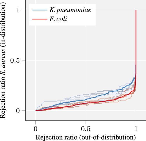
The curves depict the trade-off between in-proportion of rejected in-distribution samples versus out-of-distribution samples. A complete rejection of all out-of-distribution samples is reached at a low rejection ratio for in-training. The in-training dataset is MQ–GP–PIKE with S-AMOXCLAV

In addition, while rejecting samples with low confidences values serves to reject out-of-distribution samples, for which no informed decision can be made, it can also lead to improvements for the main classification task, namely the labelling of in-training test samples. A reliable classifier should increase its classification performance if low-confidence samples are removed. Figure 5 analyzes this by calculating the predictive performance on in-training test samples for each rejection threshold θ. We observe that the performance of both MQ–LR and MQ–GP–PIKE improves when giving the classifier the possibility to reject low-confidence samples. However, LR benefits less from low-confidence rejection in terms of prediction accuracy, and we observe a large decrease in performance in the region of high rejection thresholds ($\theta >0.95$). This suggests that some test samples received a high class probability—close to 1.0—which were in fact labelled incorrectly, which further underscores our two earlier observations, namely that (i) due to bad splits, instances are present in the testing data that are not represented in the training data distribution, and (ii) instances outside the in-training distribution receive an MCP value of $\approx 1.0$, making this classifier unsuitable for clinical applications.

Fig. 5.

The improvement in terms of prediction accuracy for every threshold θ, for S-AMOXCLAV. To permit comparability, we report the accuracy as the class ratio changes for different values of θ. Small sample size effects increase variance for larger values of θ

4 Conclusion

We developed a novel approach for antimicrobial resistance classification from MALDI-TOF mass spectra. By using a GP classifier, our method is specifically designed to stay reliable in the face of real-world clinical prediction challenges, such as the task of labelling unseen bacterial isolates. Using the presented novel kernel—PIKE—our method outperforms traditional classification algorithms while being able to provide uncertainty estimates for its predictions. Moreover, we challenged common assumptions concerning the pre-processing and developed a novel simplified pre-processing method based on ideas from computational topology. Our work thus constitutes a crucial step towards the goal of further reducing the time to provide precise antimicrobial treatments for patients while reducing the prescription of ineffective antibiotics. We hope that this will encourage additional method development for antimicrobial resistance prediction based on MALDI-TOF mass spectra.

Future work. Further assessment of the influence of pre-processing parameters on antimicrobial phenotype prediction is needed. Moreover, the utility of our confidence analysis could also be analyzed in additional scenarios of the clinical practice. Presenting the classifier with isolates collected at different geographical locations would allow to simulate infections contracted outside the local bacteria population, such as infections caught during travel. Additional experiments, such as the comparison of isolates characterized by both DNA sequencing and MALDI-TOF MS, could provide insights into how phylogenetic differences are contained in MALDI-TOF MS spectra and whether they can be recovered. The gained insights could lead to new approaches for improving the train–test split or the reformulation of separate prediction problems for different evolutionary strains.

References

- Belkin M., Niyogi P. (2002) Laplacian eigenmaps and spectral techniques for embedding and clustering. Adv. Neural Inform. Process. Syst., 14, 585–591. [Google Scholar]
- BioMérieux (2018) https://www.biomerieux.com (15 January 2020, date last accessed).
- Borgwardt K.M. (2011) Kernel methods in bioinformatics In Handbook of Statistical Bioinformatics. Springer, pp. 317–334. [Google Scholar]
- Brouard C. et al. (2016) Fast metabolite identification with input output kernel regression. Bioinformatics, 32, i28–i36. [DOI] [PMC free article] [PubMed] [Google Scholar]
- Cassini A. et al. (2019) Attributable deaths and disability-adjusted life-years caused by infections with antibiotic-resistant bacteria in the EU and the European Economic Area in 2015: a population-level modelling analysis. Lancet Infect. Dis., 19, 56–66. [DOI] [PMC free article] [PubMed] [Google Scholar]
- Chen J.H.K. et al. (2015) Use of MALDI Biotyper plus ClinProTools mass spectra analysis for correct identification of Streptococcus pneumoniae and Streptococcus mitis/oralis. J. Clin. Pathol., 68, 652–656. [DOI] [PubMed] [Google Scholar]
- Cohen-Steiner D. et al. (2007) Stability of persistence diagrams. Stability of persistence diagrams. Discrete Comput. Geom., 37, 103–120. [Google Scholar]
- Daltonics B. (2018) https://www.bruker.com (15 January 2020, date last accessed).
- De Bruyne K. et al. (2011) Bacterial species identification from MALDI-TOF mass spectra through data analysis and machine learning. Syst. Appl. Microbiol., 34, 20–29. [DOI] [PubMed] [Google Scholar]
- Dührkop K. et al. (2015) Searching molecular structure databases with tandem mass spectra using CSI: FingerID. Proc. Natl. Acad. Sci. USA, 112, 12580–12585. [DOI] [PMC free article] [PubMed] [Google Scholar]
- Edelsbrunner H., Harer J. (2010) Computational Topology: An Introduction. American Mathematical Society, Providence, RI, USA. [Google Scholar]
- EUCAST (2018) The European Committee on Antimicrobial Susceptibility Testing (EUCAST): clinical breakpoints and dosing of antibiotics. http://www.eucast.org/clinical_breakpoints/ (15 January 2020, date last accessed).
- Fangous M.-S. et al. (2014) Classification algorithm for subspecies identification within the Mycobacterium abscessus species, based on matrix-assisted laser desorption ionization–time of flight mass spectrometry. J. Clin. Microbiol., 52, 3362–3369. [DOI] [PMC free article] [PubMed] [Google Scholar]
- Feragen A. et al. (2015) Geodesic exponential kernels: when curvature and linearity conflict. In: CVPR, pp. 3032–3042. Massachusetts, USA. [Google Scholar]
- Gibb S. (2019) MALDIquant: quantitative analysis of mass spectrometry data. https://cran.r-project.org/web/packages/MALDIquant/vignettes/MALDIquant-intro.pdf (15 January 2020, date last accessed).
- Gibb S., Strimmer K. (2012) MALDIquant: a versatile R package for the analysis of mass spectrometry data. Bioinformatics, 28, 2270–2271. [DOI] [PubMed] [Google Scholar]
- Heinonen M. et al. (2012) Metabolite identification and molecular fingerprint prediction through machine learning. Bioinformatics, 28, 2333–2341. [DOI] [PubMed] [Google Scholar]
- Ho P.-L. et al. (2017) Rapid detection of cfiA metallo-β-lactamase-producing Bacteroides fragilis by the combination of MALDI-TOF MS and CarbaNP. J. Clin. Pathol., 70, 868–873. [DOI] [PubMed] [Google Scholar]
- Mather C.A. et al. (2016) Rapid detection of vancomycin-intermediate Staphylococcus aureus by matrix-assisted laser desorption ionization–time of flight mass spectrometry. J. Clin. Microbiol., 54, 883–890. [DOI] [PMC free article] [PubMed] [Google Scholar]
- Papagiannopoulou C. et al. (2019) Investigating time series classification techniques for rapid pathogen identification with single-cell MALDI-TOF mass spectrum data. In ECML PKDD, Würzburg, Germany.
- Pedregosa F. et al. (2011) Scikit-learn: machine learning in Python. J. Mach. Learn. Res., 12, 2825–2830. [Google Scholar]
- Rasmussen C.E., Williams C.K.I. (2006) Gaussian Processes for Machine Learning. MIT Press, MA, USA. [Google Scholar]
- Reininghaus J. et al. (2015) A stable multi-scale kernel for topological machine learning. In: CVPR, 4741–4748. Massachusetts, USA. [Google Scholar]
- Roe J. (1988) Elliptic Operators, Topology and Asymptotic Methods, 2nd edn Chapman & Hall/CRC, FL, USA. [Google Scholar]
- Schölkopf B. et al. (2004) Kernel Methods in Computational Biology. MIT Press, MA, USA. [Google Scholar]
- Shen H. et al. (2014) Metabolite identification through multiple kernel learning on fragmentation trees. Bioinformatics, 30, i157–i164. [DOI] [PMC free article] [PubMed] [Google Scholar]
- Sogawa K. et al. (2017) Rapid discrimination between Methicillin-sensitive and Methicillin-resistant Staphylococcus aureus using MALDI-TOF mass spectrometry. Biocontrol Sci., 22, 163–169. [DOI] [PubMed] [Google Scholar]
- Vervier K. et al. (2015) Benchmark of structured machine learning methods for microbial identification from mass-spectrometry data. Preprint, arXiv:1506.07251.
- Wang H.-Y. et al. (2018) A new scheme for strain typing of Methicillin-resistant Staphylococcus aureus on the basis of matrix-assisted laser desorption ionization time-of-flight mass spectrometry by using machine learning approach. PLoS One, 13, e0194289. [DOI] [PMC free article] [PubMed] [Google Scholar]
- Weis C.V. et al. (2020) Machine learning for microbial identification and antimicrobial susceptibility testing on MALDI-TOF mass spectra: a systematic review. Clin. Microbiol. Infect. [DOI] [PubMed] [Google Scholar]
- Zhan X. et al. (2015) Kernel approaches for differential expression analysis of mass spectrometry-based metabolomics data. BMC Bioinformatics, 16, 77. [DOI] [PMC free article] [PubMed] [Google Scholar]