Inference of population admixture network from local gene genealogies: a coalescent-based maximum likelihood approach

Abstract

Motivation

Population admixture is an important subject in population genetics. Inferring population demographic history with admixture under the so-called admixture network model from population genetic data is an established problem in genetics. Existing admixture network inference approaches work with single genetic polymorphisms. While these methods are usually very fast, they do not fully utilize the information [e.g. linkage disequilibrium (LD)] contained in population genetic data.

Results

In this article, we develop a new admixture network inference method called GTmix. Different from existing methods, GTmix works with local gene genealogies that can be inferred from population haplotypes. Local gene genealogies represent the evolutionary history of sampled haplotypes and contain the LD information. GTmix performs coalescent-based maximum likelihood inference of admixture networks with inferred local genealogies based on the well-known multispecies coalescent (MSC) model. GTmix utilizes various techniques to speed up the likelihood computation on the MSC model and the optimal network search. Our simulations show that GTmix can infer more accurate admixture networks with much smaller data than existing methods, even when these existing methods are given much larger data. GTmix is reasonably efficient and can analyze population genetic datasets of current interests.

Availability and implementation

The program GTmix is available for download at: https://github.com/yufengwudcs/GTmix.

Supplementary information

Supplementary data are available at Bioinformatics online.

1 Introduction

Population demographic history is a complex interplay of various processes, such as population divergence and isolation, population size changes, migration and admixture. The simplest population demographic history model is the population tree model (similar to phylogenetic tree for species evolution on the high level), which only models population divergence. In practice, however, the population tree model is often too simplistic for most population genetic study. One key missing aspect of the population tree model is gene flow. In this article, we focus on population admixture, which is one of the most important types of gene flow. Population admixture is often so widespread that admixture has to be addressed in most demographic history studies. Human populations for example are known to be strongly influenced by admixture throughout the human history (Patterson et al., 2012; Price et al., 2007). When admixture is considered, population history becomes a network (called admixture network). In addition to modeling population divergence, admixture network has admixture nodes that model admixture events. See Figure 1a for an illustration of admixture network.

Fig. 1.

Illustration of admixture network. (a) An admixture network. Four populations. C is admixed. (b) and (c) Two population trees in this network. (d) and (e) Two gene genealogies, each from a different loci. Leaves of gene genealogies: population haplotypes. Two sampled haplotypes per population: haplotypes a₁ and a₂ are from the population A, haplotypes b₁ and b₂ are from the population B and so on. Darkened dots: mutations (following infinite sites model). (f) Haplotypes for the two genealogies

As demographic history is not directly observable, it is highly desirable to infer population history with admixture (i.e. admixture network) from extant population genetic data (Lipson et al., 2013; Pickrell and Pritchard, 2012). Inferring admixture networks from population genetic data is challenging computationally. First, the space of admixture networks can be very large even for moderate number (say ten) of populations and small number (say two) of admixture events. There are over 34 million rooted binary trees with ten taxa. With admixture, the number of possible networks is very large (see, e.g. Cardona and Zhang, 2020). Moreover, the effect of admixture on population genetic data is subtle and is not easily detectable. Meiotic recombination further complicates the situation by breaking the linkage between genetic polymorphisms.

A natural population genetic model for admixture network inference is the coalescent model (Kingman, 1982). Coalescent process determines stochastically how sampled alleles coalesce in a population. As there are multiple populations in an admixture network, the underlying coalescent is the multispecies coalescent (MSC). MSC is the fundamental genetic model for the study of multiple closely related populations (species) (Rosenberg, 2002). MSC can be extended to allow gene flow (see, e.g. Yu et al., 2012). Under the MSC model, one can (at least in principle) perform likelihood-based inference of admixture networks. However, inference based on MSC is computationally intensive (Rosenberg, 2002). Therefore, existing methods for inferring admixture networks usually perform inference with allele frequencies at individual polymorphic sites on somewhat simplified genetic models. For example, the TreeMix approach (Pickrell and Pritchard, 2012) infers admixture networks from allele frequency data based on a Gaussian approximation of genetic drift. MixMapper (Lipson et al., 2013), another method for network inference, has similar high-level approach as TreeMix. Both TreeMix and MixMapper are fast to handle large genetic data and can be useful for admixture network inference. However, there are several downsides of these existing methods. First, only working with allele frequencies at individual polymorphisms may potentially lose information, especially the linkage disequilibrium (LD) among nearby sites. Moreover, these approaches are based on approximations of the underlying genealogical process, which may not very accurately model the MSC process. Our experience indicates that TreeMix and MixMapper, while useful, do not provide very accurate inference results in some of our simulations.

In this article, we present a new method for inferring admixture networks from population genetic data. Our new method is named GTmix (which stands for Gene Tree-based admixture network inference). The following summarizes the main features of GTmix.

1. GTmix works with haplotypes, rather than individual polymorphisms. This allows GTmix to exploit the LD information in genetic data, which is not considered by TreeMix and MixMapper. GTmix does not directly perform inference from haplotypes. Instead, GTmix takes input in the form of gene genealogies $\mathcal{T}=(T_1,T_2,\dots ,T_m)$ that are inferred from the given haplotypes. Here, T_i is the inferred gene genealogy at a site s_i, which represents the evolutionary history of haplotypes at s_i. Due to recombination, genealogies at different loci may be different. Gene genealogy is arguably more informative than individual genetic polymorphisms. Even though a genealogy T_i is only for a specific site s_i, genealogies at nearby sites tend to be similar and thus implicitly contain the LD information. A traditional view in population genetics is that while gene genealogy is informative, there is little power in inferring gene genealogies from genetic data largely due to recombination (see, e.g. Wilson and McVean, 2006). Recently, however, local genealogy inference is being actively studied and applied in population genetics. There are several existing tools for inferring gene genealogies from population haplotypes (Kelleher et al., 2019; Mirzaei and Wu, 2017; Rasmussen et al., 2014; Speidel et al., 2019). Among these tools, RENT+ (Mirzaei and Wu, 2017; Wu, 2011) is efficient and easy to use. So we use RENT+ for local genealogy inference in this article.

2. GTmix is a maximum likelihood approach: it aims at finding an admixture network ${\mathcal{N}}_{\text{opt}}$ such that $\text{Pr}(\mathcal{T}|{\mathcal{N}}_{\text{opt}})$ is maximized. Here, $\text{Pr}(\mathcal{T}|\mathcal{N})=\prod _{i=1}^m\mathrm{P}\mathrm{r}(T_i|\mathcal{N})$ (based on the assumption the independence of each T_i). $\text{Pr}(T_i|\mathcal{N})$ is the probability of observing the genealogy T_i for the admixture network $\mathcal{N}$ under the MSC with admixture (MSCA) model. In general, computing $\text{Pr}(\mathcal{T}|\mathcal{N})$ under the MSCA model is computationally challenging. Building on the recent algorithmic progress in efficient probability computation on the MSC model (Pei and Wu, 2017; Wu, 2012, 2016), GTmix implements several approaches to speed-up the likelihood computation on the MSCA model. By working on the MSCA model, GTmix performs admixture network inference on an arguably more rigorous model than existing methods (such as TreeMix).

3. GTmix can be configured to infer admixture networks with arbitrary number of admixture events, although the running time will be longer with larger number of admixture events. It can infer recent admixture (i.e. that forms an extant population) and also ancient admixture (i.e. that forms an ancestral population). GTmix is reasonably efficient computationally. In phylogenetics, there exists methods [most notably the program Phylonet (Wen et al., 2018)] for inferring phylogenetic networks (somewhat related to admixture networks) based on the MSCA model. Our experience indicates that GTmix can perform likelihood-based inference on data with significantly larger number of taxa and haplotypes than what are allowed by existing approaches such as Phylonet.

Through simulation, we show that while GTmix is not as fast as existing methods such as TreeMix, GTmix is more accurate than existing methods in most simulations we performed. In particular, GTmix can infer more accurate admixture networks under most settings using much smaller data than existing methods, even when those existing methods use much larger data than GTmix. Our results suggest that inferred genealogies can indeed be informative for population demographic history inference. Also coalescent-based probabilistic inference with local genealogies can potentially be more accurate than existing methods using single polymorphisms.

2 Background

2.1 Admixture network

Admixture network is conceptually similar to phylogenetic network as studied in the Phylogenetics literature (Huson et al., 2010; Morrison, 2011). Admixture network is a natural extension to the population tree model (see, e.g. Wu, 2015). Admixture network (or simply network) is a directed acyclic graph $\mathcal{N}$, and is leaf-labeled by a set of populations. Moreover,

1. Admixture nodes are nodes in $\mathcal{N}$ with two incoming edges. The two ancestral nodes of an admixture node are called the source populations.

2. For a network $\mathcal{N}$, when only one of the incoming edges of each admixture node is kept and the other is deleted, we always obtain a tree T. This tree is called the population tree. There can be multiple populations trees contained in a network.

Note that in admixture network, a node refers to a population. An admixed node has two incoming edges, which originate from two source populations of the admixed population. Thus, for an admixture node v in a network, there are two ancestral nodes: the left parent [denoted as Left(v)] and the right parent [denoted as Right(v)]. Throughout this article, we assume each admixture is two-way (i.e. formed by two ancestral populations). More general admixture (involving three or more ancestral populations) can in principle be modeled as a chain of two-way admixture events.

Population tree. Recall that a population tree T is contained in a network $\mathcal{N}$ when we remove one of the two incoming edges at each admixture node. Suppose there are n_a admixture nodes in $\mathcal{N}$. There are $2^{n_{\mathrm{a}}}$ population trees contained in $\mathcal{N}$. For example, in Figure 1, there are two population trees contained in the network, as shown in Figure 1d and e. Note that population trees do not capture all the possible demographic histories in $\mathcal{N}$. This is because population tree assumes that all lineages from an admixed population follow either the left or right admixture branches when coalescing at a locus. But this is not necessarily the case at an admixture event. Despite this shortcoming, GTmix relies on population trees for likelihood computation because it is computationally more efficient to work with population trees than with a network.

Branch length. Branches in a network have lengths in the standard coalescent units. In this article, we assume population sizes remain constant within a single branch of $\mathcal{N}$. Note that different branches may have different population sizes. The admixture network model accommodates this using the standard coalescent unit (which converts the absolute time to the number of generations based on the effective population size) for branch lengths in the network, rather than the absolute time.

Admixture proportions. At each admixture node v, there is an admixture proportion $f_0(v)$ where $0\le f_0(v)\le 1$. $f_0(v)$ refers to the proportion of alleles of population v originating from the left parent Left(v). $f_1(v)=1.0-f_0(v)$ is the proportion of alleles of v from the right parent.

Genealogy and multispecies coalescent. Gene genealogy and MSC are central to GTmix. Due to the lack of the space, relevant background information is given in Supplementary Materials.

3 Materials and methods

3.1 The high-level approach of GTmix

We assume haplotypes $\mathcal{H}$ from n_p populations are given. We further assume the number of admixture events n_a is known. Note that, this is a standard assumption in existing admixture network inference literature. Our goal is inferring the maximum likelihood admixture network $\mathcal{N}$ with n_a admixture nodes for these populations from $\mathcal{H}$. One natural approach is finding $\mathcal{N}$ that maximizes the likelihood $P(\mathcal{H}|\mathcal{N})$ of $\mathcal{H}$. However, computing $P(\mathcal{H}|\mathcal{N})$ is challenging. GTmix uses the following techniques to develop a practical coalescent-based maximum likelihood inference approach.

1. GTmix works with local genealogies $\mathcal{T}$ (which are inferred from $\mathcal{H}$), instead of with $\mathcal{H}$ directly. Before using GTmix, we first use a local genealogy inference tool [e.g. RENT+ (Mirzaei and Wu, 2017)] to infer local gene genealogies $\mathcal{T}$ from $\mathcal{H}$. The main benefit of working with inferred genealogies is that computing the likelihood of $\mathcal{T}$ is easier than directly computing the likelihood of $\mathcal{H}$ for $\mathcal{N}$. Also local genealogies $\mathcal{T}$, while noisy, capture the important LD information. The number of local genealogies can be very large in practice. GTmix uses a filtering scheme to choose possibly more reliable gene genealogies for inference.

2. GTmix infers ${\mathcal{N}}_{\text{opt}}$ that maximizes $\text{Pr}(\mathcal{T}|{\mathcal{N}}_{\text{opt}})$. $\text{Pr}(\mathcal{T}|\mathcal{N})$ is computed approximately. That is for each $T\in \mathcal{T}$, Pr(T) is computed by summing up the (weighted) probability of T for each population tree in $\mathcal{N}$. The probability of T for a population tree is computed using the fast algorithm in Pei and Wu (2017) that computes gene tree probability approximately. GTmix implements effective methods to perform network search, including a new method for constructing initial networks from gene genealogies.

3.2 Inferring local gene genealogies

For local genealogy inference from haplotypes, GTmix is tested with genealogies inferred by the program RENT+ (Mirzaei and Wu, 2017), although other tools (e.g. Kelleher et al., 2019; Speidel et al., 2019) can be used as well. RENT+ infers a (rooted binary) genealogy for each binary polymorphic site within a locus. The total number of local genealogies can be very large because there can be a different genealogy at each site. This makes it infeasible to perform likelihood-based inference with all genealogies as computing the probability of a genealogy is not trivial. To develop a practical method, GTmix samples a subset of genealogies (trees) using a two-stage approach: (i) it first chooses a subset of (likely more reliable) trees from inferred trees at each locus and (ii) it then chooses a smaller subset of trees from the list of trees from all loci. Note that, we assume haplotypes are divided into (independent) regions (loci), where each locus can contain many polymorphic sites.

3.2.1 Choosing genealogies from each locus

GTmix uses the following simple method called TreePicker for picking a subset of gene genealogies from potentially a large number of local genealogies inferred by RENT+. TreePicker works with haplotypes ${\mathcal{H}}_i$ from the ith locus and a list of genealogical trees ${\mathcal{T}}_i$ inferred by RENT+ from ${\mathcal{H}}_i$. TreePicker chooses a fixed number n_T trees from ${\mathcal{T}}_i$ as follows.

1. TreePicker first divides the polymorphic sites within the ith locus into n_T equal-sized segments.

2. For each segment, TreePicker chooses one genealogy $T_i\in {\mathcal{T}}_i$ which ‘matches’ the largest number of polymorphisms within this segment.

Recall that a (binary) polymorphic site implies a split (bipartition) of sampled haplotypes under the infinite sites model. We say a tree T matches a polymorphic site if there is a clade of T whose leaves are exactly those on one side of the split implied by this site. While local genealogies inferred by RENT+ do have useful information, these trees also have significant noise. Intuitively, an inferred genealogy T tends to be more reliable if it matches more polymorphic sites. This is because polymorphic sites are given as input and presumably correspond to clades in gene genealogies. A local genealogy is likely more reliable if it matches more polymorphisms.

3.2.2 Choosing a subset of trees to use for inference

GTmix takes a list of trees chosen by TreePicker as input. The number of input trees can still be large, and these genealogies can still be noisy. Before GTmix starts the inference, it first chooses a subset of up to K trees (by default, K = 500) from the input trees. The basic idea is removing input trees that are significantly different from the rest of trees. This is because such trees are more likely to contain errors. GTmix takes the following simple approach for choosing trees for inference. It first analyzes input trees and calculates the frequencies of the clades in the trees. Then, it scores a tree by clade frequencies: a tree T is assigned a score $\prod _{C\in \text{Clades}(T)}\mathrm{f}\text{req}(C)$. Here, Clades(T) is the set of all clades of the tree T and freq(C) is the estimated frequency of the clade C in all trees. GTmix chooses up to K trees with the highest scores. The main rationale behind this tree-picking step is that the number of true genealogical trees within a region is likely to be relatively small. This is because the number of recombinations (and other population demographic events such as admixture and incomplete lineage sorting) within a small region is likely small. Thus, a local genealogy is likely to be more reliable if it shares more topological features with other genealogies.

3.3 Gene tree probability computation for admixture network

GTmix takes a list of inferred genealogies $\mathcal{T}=\{T_1,\dots ,T_K\}$ as input. The most important aspect for inferring admixture network $\mathcal{N}$ is computing $P(\mathcal{T}|\mathcal{N})$ under the multispecies coalescent with admixture (MSCA) model. Assuming the independence of genealogies, $P(\mathcal{T}|\mathcal{N})={\prod }_{i=1}^{K}P(T_i|\mathcal{N})$. Computing $P(T_i|\mathcal{N})$ for a network $\mathcal{N}$ is not trivial (see, e.g. Yu et al., 2012). The main difficulty for computing $P(T_i|\mathcal{N})$ is that the number of feasible coalescent histories can be very large under the MSCA model. To develop a practical method that can work with relatively large data, GTmix takes an approximation here: instead of computing the probability of T_i for $\mathcal{N}$, GTmix computes the probability of each population tree T_i in $\mathcal{N}$ and then use a weighted sum of these probability as an approximation of $P(T_i|\mathcal{N})$. While this is only an approximation, our experience indicates this allows reasonably accurate and efficient inference of admixture network.

To be specific, we consider all possible population trees in $\mathcal{N}$. Each population tree is obtained by picking one of the left and right admixture edges at admixture node v with probabilities m_v and $1.0-m_v$, respectively. Let the embedded population trees within $\mathcal{N}$ be ${\mathcal{T}}_{\mathcal{N}}=\{T_{\mathcal{N},1},\dots ,T_{\mathcal{N},k}\}$. Let n_a be the number of admixture nodes in $\mathcal{N}$. A population tree $T_{\mathcal{N},j}$ is associated with a binary vector D_j of length n_a. $D_j[a]=0$ ($D_j[a]=1$, respectively) if the left (right, respectively) incoming edge is chosen to obtain $T_{\mathcal{N},j}$. Here, each $T_{\mathcal{N},j}$ has a probability of being the population tree: $P(T_{\mathcal{N},j})={\prod }_{i=1}^{n_a}{m}_{v_i}^{1-D_j(i)}{(1-m_{v_i})}^{D_j(i)}$. Here, v_i is the ith admixture node. Recall that branches in $\mathcal{N}$ have lengths. Trees in ${\mathcal{T}}_N$ are derived from $\mathcal{N}$ and so have branch lengths too. In contrast, we assume genealogical trees in $\mathcal{T}$ are topologies only [as assumed in Rosenberg (2002) and Degnan and Salter (2005)]. Thus,

$$P(T_i|\mathcal{N})\approx \sum _{j=1}^{2^{n_a}}P(T_{\mathcal{N},j})P(T_i|T_{\mathcal{N},j})$$ (1)

$P(T_i|T_{\mathcal{N},j})$ is exactly the gene tree probability of a gene tree topology for a fixed population tree with branch lengths (Degnan and Salter, 2005; Rosenberg, 2002). GTmix uses the approximate gene tree probability algorithm in Pei and Wu (2017). This is because this algorithm is much more scalable than exact gene tree probability algorithms in Degnan and Salter (2005) and Wu (2012, 2016). Note that even we had computed the exact $P(T_i|T_{\mathcal{N},j})$, Equation 1 is still only an approximation. This is because Equation 1 implicitly assumes all lineages at an admixture node are inherited from a single parent. This may not be the case with admixture. To see this, we again look at the network in Figure 1a and the gene tree in Figure 1d. Suppose at the time of admixture, lineages c₁ and c₂ remain un-coalesced. Then, Equation 1 ignores the situation where for example c₁ is from the left and c₂ is from the right. We adopt this approximation because: (i) computing gene tree probability for a population tree is much faster than computing gene tree probability for a network and (ii) empirical tests suggest that this approximation appears to provide reasonably accurate inference.

3.4 Finding the maximum likelihood admixture network

GTmix finds the maximum likelihood admixture network with n_a admixture events (where n_a is assumed to be known) using a simple iterative procedure:

1. Construct an initial network ${\mathcal{N}}_{\text{init}}$ with n_a admixture nodes from the inferred gene genealogies $\mathcal{T}$. Let ${\mathcal{N}}_{\text{opt}}\leftarrow {\mathcal{N}}_{\text{init}}$.

2. Find the set of admixture networks $\mathcal{S}$ that are similar topologically to ${\mathcal{N}}_{\text{opt}}$ and have n_a admixture nodes.

3. Let $\mathcal{N}\in \mathcal{S}$ that maximizes the likelihood $P(\mathcal{T}|\mathcal{N})$. If $P(\mathcal{T}|\mathcal{N})>P(\mathcal{T}|{\mathcal{N}}_{\text{opt}})$, set ${\mathcal{N}}_{\text{opt}}\leftarrow \mathcal{N}$, and go to step 2. Otherwise, stop.

3.4.1 Constructing the initial network

GTmix constructs an initial network ${\mathcal{N}}_{\text{init}}$ from $\mathcal{T}$ as follows. It first constructs a network ${\mathcal{N}}_0$ without admixture nodes (i.e. a population tree) by neighbor joining (NJ). The detailed procedure is given in Supplementary Algorithm S1 (in Supplementary Materials). To run the NJ algorithm, GTmix first estimates the pairwise distance between each pair of populations p_i and p_j based on $\mathcal{T}$. Intuitively, if haplotypes from two populations are closely related in a genealogy, this offers a hint that these two populations may be closely related in the admixture network. More specifically, the pairwise population distance between p_i and p_j is estimated based on the average distance between one haplotype from p_i and one from p_j (in terms of the number of edges separating these two haplotypes on an inferred genealogy). Note that, a haplotype corresponds to a leaf in $\mathcal{T}$.

GTmix then adds n_a admixture nodes to ${\mathcal{N}}_0$ by choosing proper leaf nodes in ${\mathcal{N}}_0$ and turning them into admixture nodes. That is the initial admixed populations are extant populations in ${\mathcal{N}}_0$. Note that ancestral admixture events (i.e. admixture at ancestral populations) are accommodated during the network search stage. GTmix relies on the so-called minimum deep coalescent (MDC) (Maddison, 1997; Page and Charleston, 1997) to identify likely admixed extant populations. Briefly, MDC is a statistic that measures the topological deviation of the given gene trees from a consensus tree based on the MSC model. Refer to the studies by Page and Charleston (1997) and Maddison (1997) for more details on MDC. While MDC is known to have issues in phylogenetics (see, e.g. Felsenstein, 2004), we use MDC due to its simplicity and efficiency.

The key idea of GTmix for identifying the likely admixed extant populations from $\mathcal{T}$ is that admixed extant populations tend to make gene genealogies deviate significantly from the standard MSC process. Intuitively, an admixed population tends to lead to gene genealogies that are quite different from those arising from the standard MSC process. Suppose we discard all haplotypes from the admixed population in the gene genealogies. The (reduced) gene genealogies tend to have a better fit to the standard MSC process. GTmix uses the MDC statistic to measure how well gene genealogies fit the standard MSC process. More specifically, suppose a population p is a candidate for admixed extant population. We first compute the MDC score (denoted as MDC) of the original $\mathcal{T}$. Then we discard all gene lineages from the population p in all trees of $\mathcal{T}$. We call the reduced genealogies $\mathcal{T}\prime$. We then compute the MDC score (denoted as MDC_p) on $\mathcal{T}\prime$. As each tree in $\mathcal{T}\prime$ is a subtree of the corresponding tree in $\mathcal{T},\hspace{0.17em}{\text{MDC}}_{\mathrm{p}}\le \text{MDC}$. We expect $\text{MDC}-{\text{MDC}}_{\mathrm{p}}$ for admixed population p to be significantly larger than $\text{MDC}-{\text{MDC}}_{{\mathrm{p}}_0}$ for an un-admixed population p₀. This leads to Algorithm 1 for finding likely admixed extant populations.

Algorithm 1 Identifying likely admixed extant populations from genealogies $\mathcal{T}$

1: Let $\mathcal{P}$ be the set of all populations.

2: for$k=1\dots n_a$do

3:  Compute the MDC score (denoted as MDC) for $\mathcal{T}$.

4:   for each $p\in \mathcal{P}$do

5:   Construct reduced genealogies ${\mathcal{T}}_p$ by discarding lineages from p (and cleaning up the trees so that trees remain to be binary).

6:   Compute the MDC score (denoted as MDC_p) on ${\mathcal{T}}_p$

7:  end for

8: Let $p_a\leftarrow \mathit{argma}{x}_{p\in P}(\mathit{MDC}-MD{C}_p)$. $\mathcal{P}=\mathcal{P}-\left\{p_a\right\}$. $\mathcal{T}\leftarrow {\mathcal{T}}_{p_a}$. Add p_a to ${\mathcal{P}}_a$ (the list of likely admixed extant populations).

9: end for

Constructing initial network $\mathcal{N}$by adding admixture nodes. For each likely admixed extant population $p_{\mathrm{a}}\in {\mathcal{P}}_{\mathrm{a}}$, GTmix modifies ${\mathcal{N}}_0$ by adding one admixture branch into p_a to make p_a an admixture node. GTmix considers all possible admixture source populations that can be ancestral to p_a according to the current network. Each choice leads to a network ${\mathcal{N}}_{{\mathrm{p}}_{\mathrm{a}}}$. Then it chooses one source population that gives the maximum probability $P(\mathcal{T}|{\mathcal{N}}_{{\mathrm{p}}_{\mathrm{a}}})$. After this step, we obtain the initial network ${\mathcal{N}}_{\text{init}}$.

3.4.2 Search over the space of networks

GTmix searches for the set of topologically similar networks $\mathcal{S}$ from the current network $\mathcal{N}$. Networks in $\mathcal{S}$ are obtained by applying one nearest neighbor interchange (NNI) to the current network. More specifically, consider each branch $b=(v_{\mathrm{p}},v_{\mathrm{c}})$ in $\mathcal{N}$, where node v_p is the parent of node v_c. Let v_s be the sibling of v_c, and v_sp be the sibling of v_p. Then after applying one NNI on b, we obtain a new network with v_sp being the sibling of v_c and v_s being the sibling of v_p. That is, the NNI swaps v_s with v_sp which leads to a new network $\mathcal{N}\prime$. We perform NNI on all branches in $\mathcal{N}$ to obtain $\mathcal{S}$.

3.5 Simulation

To test the performance of GTmix, we first generate random admixture networks. Then we simulate haplotypes on these admixture networks. There are a number of parameters in the simulation, which are shown in Table 1. Each parameter has a default value.

Table 1.

A list of parameters and their default values used in the simulation

Description	Symbol	Default
Number of populations (excluding the outgroup)	n p	6
Number of admixture nodes in a network	n a	1
Time interval between events (in coalescent units)	t s	0.02
Admixture proportion at admixture node v	mv	0.5
Number of haplotypes per population	n c	4/100
Number of loci	n L	500
Mutation parameter	θ	50
Recombination parameter	ρ	50
Length of locus (in bp)	L	500 000

Note: Small data with four haplotypes per populations. Large data with 100 haplotypes per population (only for TreeMix/MixMapper).

3.5.1 Admixture network simulation

We first generate random admixture networks with n_p populations. Here, $n_{\mathrm{p}}=4,6,8$ and 10. For each n_p, we simulate 10 randomly generated networks. We add one additional population as the outgroup (our experience shows that without outgroup, TreeMix appears to perform poorly especially in network rooting.). That is, the total number of populations is $n_{\mathrm{p}}+1$. A network has n_a admixture nodes, where n_a = 1 (default) or 2. We focus on networks with more recent admixture in the simulation. In most of our simulations, we choose extant populations (leaves of a network $\mathcal{N}$) as admixed populations. This is because in many genetics study, admixture is relatively recent. See Section 4.1.6 for results on networks with more ancient admixture. We arbitrarily order internal nodes in the simulated network $\mathcal{N}$, subject to the topological constraints imposed by the network. Then, each internal node v_i (i.e. the ith node in the order) is assigned a time $t_i=i\times t_{\mathrm{s}}$ where t_s is the time interval between events. All leaf nodes have zero time. The outgroup is assigned a relatively large time t_o, which by default is 0.3. The default value of t_s is 0.02 in the standard coalescent unit. Each admixture node v is associated with an admixture proportion m_v. By default, $m_v=0.5$. See Supplementary Materials for the list of simulated networks with four and six populations.

3.5.2 Haplotype simulation

For each simulated admixture network $\mathcal{N}$, we simulate a set of haplotypes using the program ms (Hudson, 2002). For each population, we simulate n_c haplotypes. By default, n_c = 4. We simulate n_L loci for each setting. By default, n_L = 500. For each locus, we set the mutation parameter θ (by default, θ = 50), and the recombination parameter ρ (by default, ρ = 50) with region length being 500 000 base pairs. The island model with population admixture implemented in ms is used to simulate the haplotypes on a specific admixture network.

4 Results

Due to the lack of space, some results are provided in Supplementary Materials.

4.1 Results on simulated data

At present, GTmix cannot run on data with large number of populations and/or large number of haplotypes per population. Thus, we run GTmix with relatively small number of haplotypes per population (by default, four haplotypes per population). TreeMix and MixMapper are designed to work with data with relatively large number of haplotypes. For comparison, we run TreeMix and MixMapper on two settings: (i) the ‘small’ data: the same data as given to GTmix and (ii) the ‘large’ data: simulated data with much larger number of haplotypes per population (by default, 100 haplotypes per population, i.e. 25 times of the small data). Note that, the number of combinations of different parameters is very large. Therefore, when we evaluate the effect of a particular parameter, we keep all other parameters to be the default values. GTmix is run with 500 local trees by default. For smaller data, sometimes GTmix is run with 2000 local trees.

4.1.1 Metrics for benchmarking admixture network inference

In this article, we use the following two metrics for comparing the topology of the inferred network $\mathcal{N}$ and that of the true network $\mathcal{N}\prime$.

1. Best-match population tree inference error. Recall that a network $\mathcal{N}$ with n_a admixture nodes contains $2^{n_{\mathrm{a}}}$ population trees. Assuming $\mathcal{N}$ and $\mathcal{N}\prime$ have the same number of admixture nodes, we compare the $2^{n_{\mathrm{a}}}$ population trees $\mathcal{T}$ in $\mathcal{N}$ with the $2^{n_{\mathrm{a}}}$ population trees $\mathcal{T}\prime$ in $\mathcal{N}\prime$. Here, we need to match each tree $T\in \mathcal{T}$ with a tree $T\prime \in \mathcal{T}\prime$. There are $2^{n_{\mathrm{a}}}!$ ways of matching $\mathcal{T}$ with $\mathcal{T}\prime$. For example when n_a = 1, there are two ways of matching; when n_a = 2, there are 24 ways of matching. The so-called Robinson–Foulds (RF) distance is used to compare a pair of matched trees T and $T\prime$. The RF distance is equal to the number of clades (subtrees) that are in T but not in $T\prime$. The RF distance is normalized to be between 0 and 1. For each matching, we take the average RF distance of all matched pairs of trees as the inference error. We take the smallest average RF distance over all matchings as the best-match inference error.

2. Percentage of correctly inferred admixed populations. It can be biologically important to identify which populations are admixed. This is measured by the average percentage of correctly inferred admixed populations.

4.1.2 Network inference accuracy

4.1.2.1 Varying number of populations. We run GTmix, TreeMix and MixMapper on data with varying number of populations (from 4 to 10). We sample four haplotypes for each population. We also run TreeMix and MixMapper with large data (100 haplotypes per population). We sample 2000 local genealogies for 4, 6 and 8 populations, and 500 genealogies for 10 populations. Sampling more trees can somewhat increase inference accuracy, but running time is longer (see Section 4.1.5). Figure 2 shows the results. GTmix is significantly better than TreeMix and MixMapper on small data in terms of topology inference. As expected, TreeMix and MixMapper perform better on large data than on small data. Still, GTmix with small data is still more accurate in topology inference than TreeMix and MixMapper with large data in most cases. Moreover, GTmix is significantly more accurate in admixed population inference than TreeMix and MixMapper.

Fig. 2.

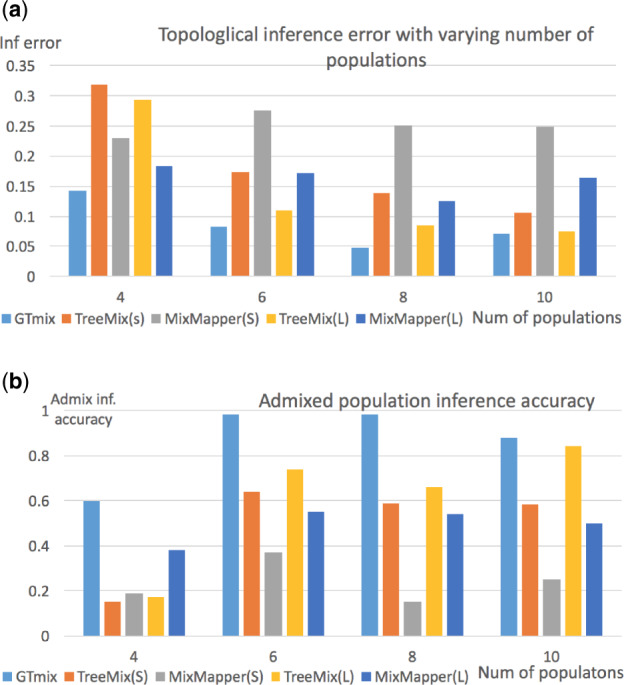
Admixture network inference with varying number of populations. GTmix: four haplotypes per population (sample 2000 trees for $n_{\mathrm{p}}=4,6$ and 8, and 500 trees for n_p = 10). TreeMix and MixMapper: small data (four haplotypes per population, denoted as ‘S’) and large data (100 haplotypes per population, denoted as ‘L’). (a) Average best-match RF distance between inferred networks and true networks. (b) Average admixture population inference accuracy. X-axis: number of populations

4.1.2.2 Varying number of haplotypes per population. We evaluate the performance of GTmix when the number of haplotypes per population varies. Six populations are simulated. Due to the computational difficulty, GTmix only runs on data with up to 8 haplotypes per population. For comparison, TreeMix and MixMapper are run on data with up to 100 haplotypes per population. Figure 3a shows the results. As expected, when the number of haplotypes increases, all methods tend to be more accurate. On the same data, GTmix is consistently better than TreeMix and MixMapper. GTmix can be more accurate with smaller data than TreeMix and MixMapper even the latter are run with much larger data. For example, the topology inference error of GTmix with 8 haplotypes per population is about 0.077, whereas the errors are about 0.11 and 0.17, respectively, for TreeMix and MixMapper with 100 haplotypes per population.

Fig. 3.

Inference with varying number of haplotypes and number of admixture events. (a) Varying number of haplotypes per population. GTmix: 2–8 haplotypes per population. That is, GTmix is not run for 10, 50 and 100 haplotypes. TreeMix and MixMapper: 2–100 haplotypes per population. X-axis: number of haplotypes (alleles) per populations. (b) With two admixture events; topological error and admixture population inference accuracy. Six populations. TreeMix is run with both small (S) and large (L) data

4.1.2.3 Two admixture events. By default, a single admixture event is simulated. To evaluate more complex demographic scenarios, we simulate two admixture events for six populations (plus one outgroup). We compare GTmix (with small data) with TreeMix (with small and large data). The results are shown in Figure 3b. We can see that GTmix outperforms TreeMix in both topological inference and admixture population inference significantly even when the latter is run with large data.

4.1.3 Phasing

So far we use the true simulated haplotypes. In practice, haplotypes are usually inferred from unphased genotypes. We now evaluate the performance of GTmix on inferred haplotypes. Note that, phasing accuracy can be affected by recombination rate. We simulate data with varying recombination rates (with the default mutation parameter of 50). We randomly pair up two simulated haplotypes to form a genotype. Then we use the program Beagle (Browning and Browning, 2007) to phase the genotypes to obtain phased haplotypes. We compare the topological inference error of networks inferred with both the true haplotypes and the phased haplotypes. The results are shown in Figure 4. When recombination rate is low, phasing error appears to have marginal effects on the inference accuracy. When recombination rate is high (say 250), there is a significant reduction in inference accuracy.

Fig. 4.

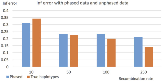
Topological inference error on phased and true haplotypes. X-axis: recombination rate used in data simulation

4.1.4 Network inference efficiency

We show the running time of GTmix under various settings in Figure 5. The running time of TreeMix and MixMapper is not shown here as these single polymorphism-based methods are much faster than GTmix. The purpose here is investigating the scalability of GTmix. The running time of GTmix apparently grows exponentially with regard to both the number of populations and the number of haplotypes per population. In contrast, GTmix scales well with regard to the number of loci. Overall, although GTmix is still computationally intensive on relatively large data, it can be applied on many data of current interests.

Fig. 5.

Running time (in seconds) of GTmix with varying number of populations, number of haplotypes per population and number of loci

4.1.5 Varying the number of genealogies for inference

The running time in Figure 5c does not grow linearly with regard to the number of loci. The main reason is that GTmix use a fixed number (K) of trees from the given set of trees in inference. Here, the default value of K is 500. The choice of K can affect both the running time and also the accuracy of GTmix. To investigate the effect of the value of K, we test GTmix with varying K values (from 100 to 5000) with six populations and four alleles per population. Figure 6 shows the results. There is a clear trade-off between inference accuracy and efficiency with regard to the number of sampled trees. Overall, larger K values tend to produce more accurate inference results, although the running time will be longer. In practice, therefore, it may be beneficial to use larger K as long as the running time remains acceptable.

Fig. 6.

Effect of the number (K) of sampled trees for inference on accuracy and running time. (a) Network topology inference error (best-match RF distance) and admixture population inference accuracy (% of correctly inferred admixed populations) with varying values of K. (b) Running time (in seconds) with varying values of K

4.1.6 Inference of ancestral admixture

We now evaluate the performance of GTmix on admixture inference of ancestral admixture events. Here, we simulate admixture networks with a single admixture event where the admixture event is ancestral to two or more extant populations. The numbers of simulated networks are three for n_p = 4, and five for n_p = 6. These networks are shown in Supplementary Materials. For each network, we simulate ten sets of haplotypes as replicates. We sample four haplotypes for each populations. For comparison, we run TreeMix with the same (small) data as GTmix and also with large data (with 100 sampled haplotypes). The topological accuracy results are shown in Table 2. In comparison with Figure 2a, both methods tend to perform less accurately for inferring ancestral admixture events than more recent admixture events. Nonetheless, our results show that GTmix outperforms TreeMix on the inference of ancestral admixture events. It appears that the accuracy of TreeMix for inferring ancestral admixture events does not show significant improvements as the data amount increases.

Table 2.

Topological inference error for networks (for 4 and 6 populations) with ancestral admixture events for GTmix and TreeMix (with 10 replicates)

	n p = 4			n p = 6
	G	T(S)	T(L)	G	T(S)	T(L)
Topology inf. error	0.20	0.37	0.29	0.30	0.34	0.35

Note: G: GTmix. T(S): TreeMix with the same data as GTmix (4 haplotypes per population). T(L): TreeMix with large data (100 haplotypes per population).

4.2 Results on the 1000 Genomes Project data

The 1000 Genomes Project (The 1000 Genomes Project Consortium, 2015) has released haplotypes of 1092 individuals from 26 populations in Phase 3 integrated variant set release. The 1000 Genomes Project defines five super populations: African, East Asian, European, South Asian and Admixed American. We pick two populations from each of these super populations. Namely, we pick the following ten populations: Americans of African Ancestry in SW USA (ASW), Yoruba in Ibadan, Nigeria (YRI), Han Chinese in Beijing, China (CHB), Japanese in Tokyo, Japan (JPT), Utah Residents with Northern and Western European Ancestry (CEU), Iberian Population in Spain (IBS), Gujarati Indian from Houston, Texas (GIH), Indian Telugu from the UK (ITU), Mexican Ancestry from Los Angeles USA (MXL) and Puerto Ricans from Puerto Rico (PUR). We create two test datasets, one small and one large. (i) The small data contain haplotypes from two randomly chosen diploid individuals (i.e. four haplotypes) from each population. We sample up to 50 loci from chromosomes 1 to 10 as follows: for each chromosome, randomly sample up to 50 regions of 100 kbp each, which are evenly located as 3 Mbp apart. (ii) The large dataset contains haplotypes from twenty diploid individuals (i.e. ten times as many as the small data) from the whole genome (i.e. all single nucleotide polymorphisms or SNPs are used). To reduce noise, any polymorphic sites with non-binary alleles are discarded.

We run GTmix to infer an admixture network with two admixture events on the small dataset only. Here, GTmix is run without specifying any outgroup. It takes about 34 h for GTmix to find the optimal network in a computer cluster (with 2.1 GHz CPU). The network is shown in Figure 7a. For comparison, we run TreeMix with the whole genome data on all 22 autosomes. Recall that GTmix is run with data from a fraction of chromosomes 1 to 10. We perform preprocessing to discard rare variants: only polymorphisms with minor allele frequencies of 5% or larger are kept (If rare alleles are kept, our simulation results show that the constructed network by TreeMix appears to be less accurate.). This leaves total 7.63 million SNPs in the data. Note that this is about 50 times more data than what is used by GTmix. Our results show that if TreeMix is run without specifying proper outgroup, the inferred network appears to be rooted in an obviously wrong position (see Supplementary Fig. S5). The resulting network by TreeMix is shown in Figure 7b, where we use YRI as the outgroup. We note that the networks inferred by GTmix and TreeMix share many key topological properties. For example, both networks have MXL and PUR as admixed. Also populations from the same super population tend to be close in the network. On the other hand, the two networks also differ in some aspects. The network by GTmix, as expected, has IBS to be closely related to the source populations involved in both inferred admixture, while the other ancestral populations involved are closely related to CHB/JPT. While the true admixture network for these populations is not known, at least some aspects of the TreeMix’s network do not agree with the commonly accepted human demographic history. For example, the TreeMix network shows MXL and PUR are both descendants from an ancestral admixture between some ancestral European and some ancestral African population; then MXL is involved in admixture with an ancestral Asian population. While MXL and PUR may have different admixture history, such ancestral admixture may not be very likely. To summarize, our results show that GTmix can provide informative inference of admixture networks on real data.

Fig. 7.

Inferred admixture network for ten populations from the 1000 Genomes Project by GTmix and TreeMix. GTmix is run with small data with two diploid individuals per population at randomly chosen regions of the first ten chromosomes, while TreeMix is run with the whole genome data with twenty diploid individuals per population (more than 50 times more data than that used by GTmix). Square box: admixture nodes (with inferred admixture proportions; the displayed admixture proportion is for the left source population). Each branch in the GTmix result has the estimated branch length (in the standard coalescent unit)

5 Conclusion and discussion

In this article, we develop a new approach called GTmix for inferring population admixture networks with local gene genealogies inferred from haplotypes. The following summarizes our findings.

1. Results of GTmix show that maximum likelihood inference of admixture networks can be practical for data that was previously believed to be not feasible (Pickrell and Pritchard, 2012). While GTmix may only find local maxima, empirical results show that GTmix can still provide reasonably accurate inference.

2. While likelihood-based inference such as GTmix is inherently more computationally demanding than existing single polymorphism-based methods, GTmix can produce more accurate inference results using only a small percentage of data than existing single polymorphism-based methods. While human populations in the 1000 Genomes Project have relatively large sample sizes, population sample sizes can be much smaller in other population genetics studies. GTmix can be useful for such datasets. Another advantage of GTmix is that its rooting of networks is usually more accurate than that of TreeMix.

GTmix builds on several published approaches (Mirzaei and Wu, 2017; Pei and Wu, 2017; Wu, 2012). The main contribution of GTmix to network inference methodology is that GTmix introduces several practical techniques that significantly speed up the computationally intensive likelihood-based network inference, and achieves reasonably good empirical performance. One common problem for GTmix and all existing admixture network inference methods is that the number of admixture events is assumed to be known. In principle, it would be useful if a method can also infer the optimal number of admixture events. Inferring the number of admixture events is a model selection problem in statistics, which is likely to be an important problem for future network inference research.

The main computational bottleneck for likelihood-based methods is still the computation of the likelihood under the coalescent process. Scaling up likelihood-based inference will need further improvement in algorithmic efficiency of coalescent likelihood computation.

Funding

This work was partly supported by U.S. National Science Foundation grants CCF-1718093 and IIS-1909425.

Conflict of Interest: none declared.

References

- Browning S.R., Browning B.L. (2007) Rapid and accurate haplotype phasing and missing data inference for whole genome association studies by use of localized haplotype clustering. Am. J. Hum. Genet., 81, 1084–1097. [DOI] [PMC free article] [PubMed] [Google Scholar]
- Cardona G., Zhang L. (2020) Counting tree-child networks and their subclasses. arXiv:1908.01917.
- Degnan J.H., Salter L.A. (2005) Gene tree distributions under the coalescent process. Evolution, 59, 24–37. [PubMed] [Google Scholar]
- Felsenstein J. (2004) Inferring Phylogenies. Sinauer, Sunderland, MA. [Google Scholar]
- Hudson R. (2002) Generating samples under the Wright-Fisher neutral model of genetic variation. Bioinformatics, 18, 337–338. [DOI] [PubMed] [Google Scholar]
- Huson D.H. et al. (2010) Phylogenetic Networks: Concepts, Algorithms and Applications. Cambridge University Press, Cambridge, UK. [Google Scholar]
- Kelleher J. et al. (2019) Inferring whole-genome histories in large population datasets. Nat. Genet., 51, 1330–1338. [DOI] [PMC free article] [PubMed] [Google Scholar]
- Kingman J.F.C. (1982) The coalescent. Stochast. Process. Appl., 13, 235–248. [Google Scholar]
- Lipson M. et al. (2013) Efficient moment-based inference of admixture parameters and sources of gene flow. Mol. Biol. Evol., 30, 1788–1802. [DOI] [PMC free article] [PubMed] [Google Scholar]
- Maddison W. (1997) Gene trees in species trees. Syst. Biol., 46, 523–536. [Google Scholar]
- Mirzaei S., Wu Y. (2017) RENT+: an improved method for inferring local genealogical trees from haplotypes with recombination. Bioinformatics, 33, 1021–1030. [DOI] [PMC free article] [PubMed] [Google Scholar]
- Morrison D.A. (2011) Introduction to Phylogenetic Networks. RJR Productions, Uppsala, Sweden. [Google Scholar]
- Page R.D.M., Charleston M.A. (1997) From gene to organismal phylogeny: reconciled trees and the gene tree/species tree problem. Mol. Phylogenet. Evol., 7, 231–240. [DOI] [PubMed] [Google Scholar]
- Patterson N. et al. (2012) Ancient admixture in human history. Genetics, 192, 1065–1093. [DOI] [PMC free article] [PubMed] [Google Scholar]
- Pei J., Wu Y. (2017) STELLS2: fast and accurate coalescent-based maximum likelihood inference of species trees from gene tree topologies. Bioinformatics, 33, 1789–1797. [DOI] [PubMed] [Google Scholar]
- Pickrell J., Pritchard J. (2012) Inference of population splits and mixtures from genome-wide allele frequency data. PLoS Genet., 8, e1002967. [DOI] [PMC free article] [PubMed] [Google Scholar]
- Price A.L. et al. (2007) A genomewide admixture map for Latino populations. Am. J. Hum. Genet., 80, 1024-1036. [DOI] [PMC free article] [PubMed] [Google Scholar]
- Rasmussen M. et al. (2014) Genome-wide inference of ancestral recombination graphs. PLoS Genet., 10, e1004342. [DOI] [PMC free article] [PubMed] [Google Scholar]
- Rosenberg N.A. (2002) The probability of topological concordance of gene trees and species trees. Theor. Popul. Biol., 61, 225–247. [DOI] [PubMed] [Google Scholar]
- Speidel L. et al. (2019) A method for genome-wide genealogy estimation for thousands of samples. Nat. Genet., 51, 1321–1329. [DOI] [PMC free article] [PubMed] [Google Scholar]
- The 1000 Genomes Project Consortium. (2015) A global reference for human genetic variation. Nature, 526, 64–74. [DOI] [PMC free article] [PubMed] [Google Scholar]
- Wen D. et al. (2018) Inferring phylogenetic networks using PhyloNet. Syst. Biol., 67, 735–740. [DOI] [PMC free article] [PubMed] [Google Scholar]
- Wilson D.J., McVean G. (2006) Estimating diversifying selection and functional constraint in the presence of recombination. Genetics, 172, 1411–1425. [DOI] [PMC free article] [PubMed] [Google Scholar]
- Wu Y. (2011) New methods for inference of local tree topologies with recombinant SNP sequences in populations. IEEE/ACM Trans. Comput. Biol. Bioinf., 8, 182–193. [DOI] [PubMed] [Google Scholar]
- Wu Y. (2012) Coalescent-based species tree inference from gene tree topologies under incomplete lineage sorting by maximum likelihood. Evolution, 66, 763–775. [DOI] [PubMed] [Google Scholar]
- Wu Y. (2015) A coalescent-based method for population tree inference with haplotypes. Bioinformatics, 31, 691–698. [DOI] [PMC free article] [PubMed] [Google Scholar]
- Wu Y. (2016) An algorithm for computing the gene tree probability under the multispecies coalescent and its application in the inference of population tree. Bioinformatics, 32, i225–i233. [DOI] [PMC free article] [PubMed] [Google Scholar]
- Yu Y. et al. (2012) The probability of a gene tree topology within a phylogenetic network with applications to hybridization detection. PLoS Genet., 8, e1002660. [DOI] [PMC free article] [PubMed] [Google Scholar]
Associated Data
This section collects any data citations, data availability statements, or supplementary materials included in this article.