Weighted minimizer sampling improves long read mapping

Abstract

Motivation

In this era of exponential data growth, minimizer sampling has become a standard algorithmic technique for rapid genome sequence comparison. This technique yields a sub-linear representation of sequences, enabling their comparison in reduced space and time. A key property of the minimizer technique is that if two sequences share a substring of a specified length, then they can be guaranteed to have a matching minimizer. However, because the k-mer distribution in eukaryotic genomes is highly uneven, minimizer-based tools (e.g. Minimap2, Mashmap) opt to discard the most frequently occurring minimizers from the genome to avoid excessive false positives. By doing so, the underlying guarantee is lost and accuracy is reduced in repetitive genomic regions.

Results

We introduce a novel weighted-minimizer sampling algorithm. A unique feature of the proposed algorithm is that it performs minimizer sampling while considering a weight for each k-mer; i.e. the higher the weight of a k-mer, the more likely it is to be selected. By down-weighting frequently occurring k-mers, we are able to meet both objectives: (i) avoid excessive false-positive matches and (ii) maintain the minimizer match guarantee. We tested our algorithm, Winnowmap, using both simulated and real long-read data and compared it to a state-of-the-art long read mapper, Minimap2. Our results demonstrate a reduction in the mapping error-rate from 0.14% to 0.06% in the recently finished human X chromosome (154.3 Mbp), and from 3.6% to 0% within the highly repetitive X centromere (3.1 Mbp). Winnowmap improves mapping accuracy within repeats and achieves these results with sparser sampling, leading to better index compression and competitive runtimes.

Availability and implementation

Winnowmap is built on top of the Minimap2 codebase and is available at https://github.com/marbl/winnowmap.

1 Introduction

Continued development of time and space-efficient algorithmic techniques has been pivotal for dealing with the exponential growth of DNA sequencing throughput. In the context of mapping and alignment applications, tools have evolved from purely alignment-based (Smith and Waterman, 1981), to seed-and-extend (Altschul et al., 1997; Kurtz et al., 2004), to succinct text indexing (Langmead and Salzberg, 2012; Yu et al., 2015) and now to ‘sketch’-based (Ondov et al., 2016; Li, 2018b) techniques. Sketch-based algorithms use dimensionality reduction to transform a sequence into a more compact representation, e.g. a subset of k-mers present in the sequence (Marçais et al., 2019; Rowe, 2019). While these algorithms continue to be widely leveraged in bioinformatics, they are even more prevalent for long-read (PacBio/Oxford Nanopore) analyses because longer strings are more amenable to compaction. As such, several long-read-based mappers (Jain et al., 2018; Li, 2016, 2018b; Popic and Batzoglou, 2017), genome assemblers (Berlin et al., 2015; Chin and Khalak, 2019; Koren et al., 2017; Kundu et al., 2019; Shafin et al., 2020, Baharav et al., 2020), metagenomic read classifiers (Dilthey et al., 2019) and transcriptomic tools (Sahlin and Medvedev, 2020; Sahlin et al., 2020) use either minimizer- or MinHash-based sequence comparison.

Minimizer sampling was introduced to the field by Roberts et al. (2004) for scaling the genome assembly problem, after being independently described a year earlier by Schleimer et al. (2003) in the text mining literature. Given a fixed window length w and a pre-defined ordering of all k-mers, minimizer sampling selects the minimum k-mer from every consecutive window (Fig. 1). Minimizers can be collected in linear time with regard to the sequence length, and matching substrings can be quickly identified as the algorithm is guaranteed to select a common minimizer for two sequences if they share an exact match of at least $w+k-1$ bases long. Further, if the ordering of k-mers is determined using a random permutation, then the expected minimizer sampling density is known to be $2/(w+1)$ (Roberts et al., 2004). Due to these properties, there exists a trade-off between sensitivity and speed when deciding the window length w.

Fig. 1.

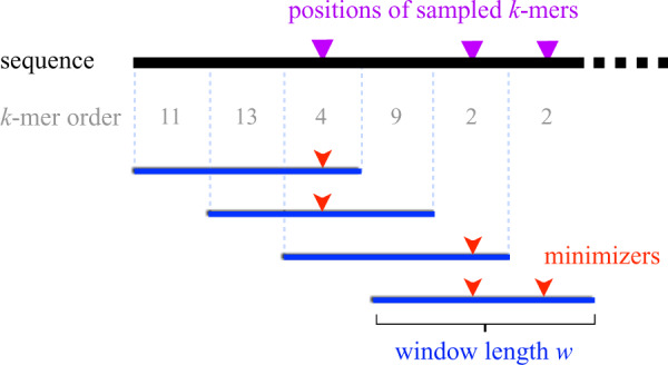
Visualization of the minimizer sampling technique (Roberts et al., 2004). The sequence being sampled is shown as a black line. Assuming a pre-defined order of k-mers (e.g. lexicographical), the sampling selects each of the smallest k-mer(s) (shown as red arrows) in consecutive sliding windows (shown as blue intervals). The length of each window, i.e. w is three in the above example

As one would expect, minimizers originating from repetitive genomic segments are sampled at a higher frequency than minimizers from unique regions. When used for seeding pairwise alignments, high-frequency minimizers lead to excessive false-positive seed hits. Examining all repetitive seed hits can prohibitively increase runtime of anchor chaining routines during the mapping process (Xin, 2018). A popular yet sub-optimal way to deal with this problem is to mask minimizers whose frequency exceeds a certain threshold. For instance, Minimap2 (Li, 2018b) discards the top 0.02% most frequently occurring minimizers, whereas Mashmap (Jain et al., 2018) discards the top 0.001% by default. An unfortunate consequence of masking is that minimizer matches are no longer guaranteed, and accuracy is reduced in repetitive genomic regions. Negative effects of k-mer masking have been highlighted before, such as poor homology detection in genomic repeats (Frith, 2011) and mis-assembly of high-copy plasmids (Koren et al., 2017).

To address the above problem, we propose optimizations to the standard minimizer sampling technique. We formulate the idea of ‘weighted-minimizers’, where k-mers that are assigned higher (or lower) weights are more (or less) likely to be selected as minimizers. Using this technique, we show that down-weighting highly repetitive k-mers avoids excessive false-positive matches, while still maintaining the guarantee that all matching substrings of length $w+k-1$ or greater will share a minimizer. The idea of using k-mer frequency to guide minimizer selection was first discussed by Chikhi et al. (2015) for a different application (further discussed in Section 1.1). In addition to weighted minimizers, we also incorporate and demonstrate the utility of ‘robust winnowing’ (Schleimer et al., 2003). In the case of multiple equally minimum k-mers in a window, robust winnowing breaks the tie by preferring a k-mer that has already been chosen by a previous window. This differs from the standard algorithm (Roberts et al., 2004), which selects all equally minimum k-mers, and is a simple yet crucial trick for efficient handling of low-complexity sequences such as ‘ACACAC…’. After implementing the above optimizations, we prove that the time complexity to compute weighted, robust minimizers remains linear with regard to sequence length and that the original minimizer match guarantee is preserved.

We refer to our implementation as Winnowmap, which replaces the minimizer sampling and indexing algorithms of the widely used alignment tool Minimap2 (Li, 2018b). In doing so, we reuse Minimap2’s highly efficient anchor chaining and gapped alignment routines. Winnowmap implements binary weights for efficiency’s sake, i.e. weights are constrained to only two possible values. We evaluate the speed and accuracy of Winnowmap using simulated and real long-read sequencing data aligned to the human reference genome GRCh38 (Schneider et al., 2017), including the recently completed X chromosome that contains the first-ever assembled human centromere (Miga et al., 2019). Compared to Minimap2, our results demonstrate that Winnowmap reduces the mapping error-rate over the entire X chromosome (0.14–0.06%), with the biggest gains achieved in the highly repetitive centromeric region (3.6–0.0%). Maintaining high alignment accuracy within long genomic repeats is critical for accurate genome assembly and variant calling. By avoiding masking, we show that Winnowmap maintains uniform minimizer density, while the masking heuristic used by Minimap2 leads to significant drops in minimizer density, especially within long tandem repeats like the centromeric satellite array. Moreover, Winnowmap uses less memory (up to 50% less) while maintaining a similar runtime versus Minimap2. Here, we focus on sequence read mapping, but we expect our optimizations to benefit all applications of minimizers.

1.1 Related work

Once a k-mer ordering is defined, the set of minimizers picked from an input sequence becomes deterministic. Accordingly, our idea of weighted-minimizers is implemented by manipulating the k-mer ordering to prefer higher weighted k-mers. There have been prior attempts to optimize minimizer selection for different applications. Chikhi et al. (2015) use frequency-based minimizer sampling for low-memory construction of de Bruijn graphs. In their implementation, a sorted frequency table of all σ^k k-mers (σ is the size of the alphabet) is computed to define a k-mer order. While sampling minimizers, a low-frequency k-mer would be selected over a high-frequency k-mer. However, this implementation does not generalize to long-read mapping applications, because there often exists a large number of erroneous low-frequency k-mers in the read set and determining an explicit order of k-mers is both difficult and unnecessary. Instead, our probabilistic approach requires storing only the set of repetitive k-mers in a reference, which is typically a much smaller set. In addition, the weighting strategy could be generalized to other criteria besides k-mer frequency, e.g. up-weighting haplotype-specific k-mers in a reference for diploid mapping.

A few works have focused on optimizing k-mer ordering to reduce the minimizer density (DeBlasio et al., 2019; Marçais et al., 2018; Orenstein et al., 2016). These optimizations are complementary to our objective as we seek to avoid excessive false-positive hits that occur by sampling high-frequency k-mers. Our formulation of weighted-minimizers is partly inspired by (Chum et al., 2008), which extends the MinHash technique to incorporate tf-idf weighting and was adopted by Canu (Koren et al., 2017) for sequence read overlap detection. Below we present background on the classic minimizer sampling (Roberts et al., 2004) and weighted MinHash (Chum et al., 2008) techniques, the two key ideas on which our algorithm is based.

2 Background

2.1 Minimizer sampling

Here, we formally discuss the standard minimizer sampling algorithm and recall its properties. Continuing the same notation, w denotes window length and σ is size of the alphabet. Let U be the universe of all σ^k k-mers, and $h:U\to [0,1]$ be a random hash function that assigns each k-mer to a real number within a unit interval. The function h induces an ordering among k-mers. Although Roberts et al. (2004) originally described the algorithm using a lexicographical ordering, a randomized ordering often works better in practice (Marçais et al., 2017).

The minimizer sampling algorithm entails computing the minimum k-mer within each consecutive window of length w. Ties are handled by picking all equally minimum k-mers (Fig. 1). Perhaps, the easiest way to compute minimizers is to use two loops such that the outer loop iterates through the input sequence while the inner loop computes a minimum k-mer within each window. Assuming the hash h of a k-mer is computable in O(1) time, this nested-loop approach requires O(nw) time for an input sequence of length n. However, there exists a linear-time O(n) algorithm for computing sliding-window minimum elements (Smith, 2011), where the trick is to use a double-ended queue while streaming k-mers (Fig. 2). This algorithm starts with an empty queue Q (Algorithm 1, line 1). Before inserting a new k-mer at the back end of Q, the algorithm scans and discards all k-mers higher than the current one (line 5). This is because all the previously seen higher k-mers cannot be minimizers of either the current or subsequent windows. Due to this step, Q maintains sorted k-mer order in each iteration. After inserting the new k-mer, we also discard those k-mers from the front that are located outside the range of the current window (line 8). Due to the sorted order in Q, the smallest k-mer is simply drawn from front of Q (line 12). Note that, each element of the array arr is inserted and deleted only once throughout the algorithm. Therefore, the total runtime of the algorithm is linear in sequence length. Schleimer et al. (2003) proved that the expected density, i.e. fraction of k-mers sampled from a random input sequence equals $2/(w+1)$. This holds true for all practical values of $w (w\ll {\sigma }^k)$ (Marçais et al., 2017).

Algorithm 1: Standard procedure for computing minimizers

Fig. 2.

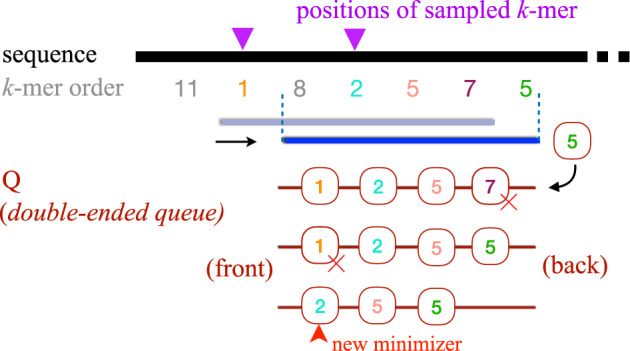
Visualizing a single iteration of Algorithm 1. As the window slides to the right, the new k-mer is inserted at the back of the double-ended queue Q, and a minimizer is selected from front end of the queue. The above figure also uses two equal k-mers (order=5) in different colours to highlight how ties are handled in Algorithm 1

We intentionally split Algorithm 1 into a main routine and four helper functions. Later when we introduce optimizations to this algorithm to avoid sampling repetitive k-mers, we will only modify the functions leaving the main routine intact. Below, we summarize the properties of the minimizer sampling Algorithm 1 as a lemma. Readers are referred to the original articles (Roberts et al., 2004; Smith, 2011) for formal proofs.

Lemma 1.

The following statements are true:

1. Algorithm 1 computes the desired set of minimizers.

2. k-mer order values in queue Q of Algorithm 1 remain sorted in non-decreasing order during execution.

3. Assuming k-mer hashing is an O(1) operation, then Algorithm 1 uses O(n) time where n is the length of input sequence.

4. If we ignore the possibility of k-mer ties within a window and assume that k-mer hash values are independent and uniformly distributed, then the expected density of minimizers is $2/(w+1)$.

5. At least one matching minimizer will be sampled from two strings with matching substrings of length $\ge w+k-1$.

2.2 MinHash and k-mer weighting

MinHash (Broder, 1997), like minimizer sampling, can be used to compute a signature of a sequence. It is a well-known locality sensitive hashing scheme for Jaccard similarity. Recall that the Jaccard similarity of two k-mer sets X and Y is $|X\cap Y|/|X\cup Y|$. Assuming k-mer hash values are independent and uniformly distributed, Broder (1997) proved that the probability of $\underset{i\in X}{\min }(h(i))=\underset{i\in Y}{\min }(h(i))$ is equal to the Jaccard similarity. This enables an unbiased estimation of Jaccard while using only a subset of the original sets. When using Jaccard, elements in $X\cap Y$ contribute uniformly to the similarity value. However, in some applications, the ‘importance’ of each element can vary. For instance, when comparing two sequences, a match of a rare k-mer carries more significance than a match of a highly repetitive k-mer. Accordingly, Chum et al. (2008) proposed a variant of the Jaccard similarity metric called weighted set-similarity. Suppose function $\mu :U\to \mathbb{N}$ assigns a weight to a k-mer, then the weighted set-similarity between two k-mer sets X and Y is given by:

$$J_w(X,Y)=\frac{\sum _{i\in X\cap Y}\mu (i)}{\sum _{i\in X\cup Y}\mu (i)}$$

Note that, $J_w(X,Y)$ is more influenced by higher-weighted k-mers. It is possible to extend the MinHash algorithm to develop an unbiased estimator for J_w. Let $h_1,h_2\dots h_{\tau }$ be τ independent random hash functions where τ equals the highest k-mer weight $\underset{i\in X\cup Y}{\max }\mu (i)$. A k-mer i is hashed using the first $\mu (i)$ hash functions: $f(i)=\underset{j=1\dots \mu (i)}{\min }{h}_j(i)$. Naturally if a k-mer has a higher weight, its expected hash value f(i) is lower because more random hashes are considered. As a result, the probability of a k-mer $i\in X$ being selected as signature of set X is decided by its weight and equals $\mu (i)/\sum _{j\in X}\mu (j)$. Thus, similar to the original MinHash algorithm, the probability of $\underset{i\in X}{\min }(f(i))=\underset{i\in Y}{\min }(f(i))$ is $J_w(X,Y)$.

In the above approach, we need to perform substantial hash evaluations to generate $\mu (i)$ uniformly distributed random numbers for each k-mer i. As a result, the above technique would require a large amount of space and time when input weights are large. Moreover, the above technique constrains the weights to be natural numbers. To remedy this, Chum et al. (2008) suggest an optimization which allows estimating J_w using a single hash evaluation for each k-mer. Their optimization follows from the observation that only the relative order of k-mer hash values matters and not their absolute values. As a result, it becomes possible to use a single random hash function while transforming its output to match the cumulative distribution of the function f. Their proposed alternative hashing function assigns k-mer i to $1-{(h_1(i))}^{1/\mu (i)}$. This also generalizes the above algorithm to real-numbered weights $\mu :U\to {ℝ}^{+}$. This algorithm partly inspired our formulation of weighted-minimizer sampling (Section 4).

3 Algorithm for robust winnowing

It is useful to recall the definition of robust winnowing:

Definition 1

(Schleimer et al., 2003). Robust winnowing: In each window, select the minimum k-mer. If possible, break ties by selecting the same k-mer as the window one position to the left. If not, select the rightmost minimal k-mer.

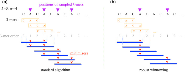
This tie breaking differs from the original algorithm of Roberts et al. (2004), which preserves all equally minimum k-mers. Robust sampling has one advantage and one disadvantage. The advantage is that we avoid sampling too many minimizers in low-complexity substrings such as ‘ACACAC…’ or ‘AAAAA…’ (Fig. 3). Its disadvantage is that the minimizer selection from a window during a tie depends on the context, i.e. it depends on which minimizers were selected in prior windows. However, our results show that the advantage outweighs the disadvantage, and this optimization yields significant improvements in runtime and memory-usage without affecting accuracy.

Fig. 3.

Visualization of tie breaking in the standard minimizer and robust winnowing algorithms. We use a low-complexity sequence ‘CACACA…’ to illustrate the difference between the two approaches. The sequence comprised two 3-mers, ‘CAC’ and ‘ACA’, which are ordered lexicographically in the above example. In the left plot, we break ties by sampling all equally minimum k-mers per window, where as we follow the robust winnowing tie breaking in the right plot. Note that robust winnowing samples half the minimizers as compared to the standard approach in this repetitive sequence example

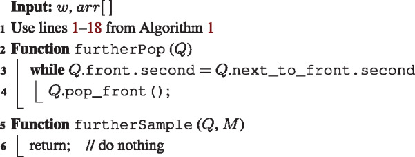
Schleimer et al. (2003) did not provide an algorithm and time complexity for computing robust minimizers, so for completeness we provide here a linear-time algorithm (Algorithm 2) that borrows psuedocode from Algorithm 1, while modifying its furtherPop and furtherSample functions. Lemma 2 proves correctness of the proposed algorithm. Similar to Algorithm 1, it is trivial to argue that the runtime remains linear. Further, any matching substring of length $\ge w+k-1$ between two sequences sample at least one robust minimizer of same order.

Algorithm 2: Computing minimizers using the robust winnowing method

Lemma 2.

Algorithm 2 computes the desired set of minimizers using the robust winnowing criteria.

Proof. Using the robust winnowing scheme, we sample a new robust minimizer at iteration i iff either of the following are true: (i) the newest k-mer is lower than all k-mers in Q, or (ii) a prior robust minimizer (i.e. the front k-mer of Q) goes out of range. In the first case, the new k-mer will be selected as a robust minimizer by the sample function and pushed to the front of Q, while discarding other k-mers in Q. In the second case, we must pick the right-most minimum k-mer if there are multiple equal minimums in Q. The function furtherPop pops all but the right-most minimum in Q. □

4 Weighted minimizer sampling

Using the same notation as before, function $\mu :U\to {ℝ}^{+}$ assigns a weight to a k-mer. Weighted minimizer sampling is defined as following.

Definition 2

Weighted minimizer sampling: Build a random ordering of all k-mers such that for a k-mer set $X=\{k_1,k_2,\dots ,k_{\left|X\right|}\}\subseteq U,\hspace{0.17em}P(k_i=\min (k_1,k_2,\dots ,k_{\left|X\right|}))=\mu (k_i)/(\mu (k_1)+\mu (k_2)+\cdots +\mu (k_{\left|X\right|}))$$\forall i\in [1,|X|]$. Using this k-mer ordering, execute the robust-winnowing procedure.

In the original minimizer sampling algorithm (Section 2.1), the k-mer ordering is defined directly using a random hash function. As a result, any k-mer in a window is equally likely to be selected as a minimizer (assuming no k-mer ties). The advantage of the weighted technique is that it allows us to bias selection of certain k-mers over others. If $(k_1,k_2,\dots k_w)$ is the set of k-mers in a window, then the probability of k-mer k_i being minimum equals $\mu (k_i)/(\mu (k_1)+\mu (k_2)+\cdots +\mu (k_w))$. As a result, the higher the weight of a k-mer relative to its neighbouring k-mers in a window, the more likely it is to be sampled as a minimizer. The weighted technique reduces to the original unweighted algorithm if all k-mer weights are equal. To define a k-mer ordering needed for weighted minimizer sampling, we borrow the optimized hashing technique of Chum et al. (2008) (Section 2.2). Given a random hash function $h:U\to [0,1]$, we assign the order of a k-mer k_i to be $1-h{(k_i)}^{1/\mu (k_i)}$.

We now analyse the expected density of weighted minimizer sampling. Recall that the expected density equals the expected fraction of k-mers sampled from a random input sequence. While the expected density using the original algorithm equals $2/(w+1)$ (Lemma 1), here the expected density depends on k-mer weights.

Lemma 3.

Suppose $k_1,k_2,\dots k_{n-k+1}$ are the k-mers in the order as they appear in a random input sequence of length n. Assume ${\sigma }^k\gg w$. The expected density of weighted minimizer sampling equals:

$$\frac{1}{n-k+1}(1+\sum _{i=1}^{n-k-w+1}\frac{\mu (k_i)+\mu (k_{i+w})}{{\sum }_{j=i}^{i+w}\mu (k_j)})$$

Proof. Suppose W_i is window of w consecutive k-mers starting at position i. Window W_i is said to be charged if the minimum k-mer in window W_i differs from the minimum k-mer in window $W_{i-1}$, i.e. W_i selects a new minimum. The expected density of a minimizer sampling can be analysed by counting total number of charged windows in the input sequence.

A union of two windows W_i and $W_{i-1}$ defines an interval of length w + 1 in the input sequence. Accordingly, k-mers $k_{i-1},k_i,\dots k_{i+w-1}$ occur in this interval, and let k_min be the minimum k-mer among these. As ${\sigma }^k\gg w$, we safely ignore the possibility of ties. Window W_i is charged if and only if either $k_{\text{min}}=k_{i-1}$ or $k_{\text{min}}=k_{i+w-1}$. Define random variable X_i to be 1 if W_i is charged and 0 if not. For $i\in [2,n-k-w+2]$ (for all windows except the first)

$$\begin{array}{c}E[X_i]=P(k_{\text{min}}=k_{i-1})+P(k_{\text{min}}=k_{i+w-1})\\ E[X_i]=\frac{\mu (k_{i-1})+\mu (k_{i+w-1})}{{\sum }_{j=i-1}^{i+w-1}\mu (k_j)}\end{array}$$

For $i=1,E[X_i]=1$. Therefore, the expected density

$$\begin{array}{c}=\frac{1}{n-k+1}(E[{\Sigma }_{i=1}^{n-k-w+2}{X}_i])\\ =\frac{1}{n-k+1}(\sum _{i=1}^{n-k-w+2}E[X_i])\\ =\frac{1}{n-k+1}(1+\sum _{i=2}^{n-k-w+2}\frac{\mu (k_{i-1})+\mu (k_{i+w-1})}{{\sum }_{j=i-1}^{i+w-1}\mu (k_j)})\\ =\frac{1}{n-k+1}(1+\sum _{i=1}^{n-k-w+1}\frac{\mu (k_i)+\mu (k_{i+w})}{{\sum }_{j=i}^{i+w}\mu (k_j)})\\ \end{array}$$

□

The theoretical worst case expected density of weighted minimizer sampling occurs when k-mers $k_1,k_2,\dots ,k_{n-k+1}$ are distinct (i.e. ${\sigma }^k\gg n$) and $\mu (k_1)\gg \mu (k_2)\gg \dots \gg \mu (k_{n-k+1})$. In this case, the density approximately equals 1. A best case scenario is one where $k_1,k_2,\dots ,k_{n-k+1}$ are distinct and weights $\mu (k_w),\mu (k_{2w}),\mu (k_{3w})\dots$ are significantly higher than all the other k-mer weights. In this case, density is optimal and equals $1/w$. It is also useful to see that if $\mu (k_1)=\mu (k_2)=\cdots =\mu (k_{n-k+1})$, then the sampling density is asymptotically equal to $2/(w+1)$. This implies that the density matches with the original algorithm within equally weighted portions of the sequence.

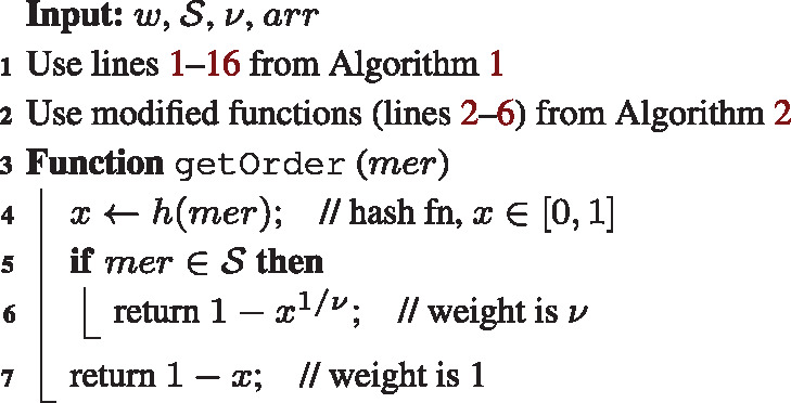
Winnowmap implements binary-weighted minimizer sampling to avoid indexing highly repetitive k-mers for long-read mapping. Given any reference genome, we assume the availability of a pre-computed set $\mathcal{S}$ of repetitive k-mers, i.e. k-mers that occur with frequency above a certain cut-off. This set can be computed efficiently using a k-mer counting tool. We assign any k-mer $k_i\in U$ a weight of $\nu <1$ if $k_i\in \mathcal{S}$, and 1 otherwise (Algorithm 3). By default, Winnowmap uses a frequency cut-off of 1024 for determining highly repetitive k-mers, and sets $\nu =1/8$. Asymptotic time complexity of minimizer sampling remains linear in sequence length if we use a σ^k-sized bit array to store the set $\mathcal{S}$ that supports membership queries in O(1) time. Here, each arithmetic operation for raising a hash value to a power (line 6) is assumed to consume constant time. If σ^k-sized bit space (34 GB for k = 19) exceeds available memory resources, a search tree data structure with $O(|\mathcal{S}|)$ space and $O(\text{log}\hspace{0.17em}|\mathcal{S}|)$ lookup time could be used instead. In practice $\left|\mathcal{S}\right|\ll {\sigma }^k$, e.g. $\left|\mathcal{S}\right|=62\hspace{0.17em}114$ with k = 19 using the human genome reference.

Algorithm 3: Algorithm for computing weighted minimizers

Lemma 4.

The following statements are true for Algorithm 3:

1. Assuming k-mer hashing is an O(1) operation, then Algorithm 3 uses O(n) time where n is length of input sequence

2. At least one minimizer of the same order will be sampled from two strings with matching substrings of length $\ge w+k-1$

Algorithm 3 involves a few computational overheads that affect indexing performance in practice. First, random accesses in a σ^k-sized bit array in each iteration make the implementation slow (line 5). Second, computing a power arithmetic operation for each occurrence of repetitive k-mers is expensive (line 6). We implement a few optimizations to avoid these overheads. We use a space-efficient bloom filter to query membership in $\mathcal{S}$, which incurs a marginal false-positive rate. For the second issue, we compute $x^{1/\nu }$ without using a power operation. For example, if ν is 1/8, then $x^{1/\nu }=x^8$ can be computed using three multiplications. Finally, we use $-x^{1/\nu }$ and –x (lines 6 and 7) to assign k-mer order values instead of $1-x^{1/\nu }$ and $1-x$, respectively, to avoid rounding errors (e.g. $1-1$e-20 rounded to 1). As a result of these optimizations, weighted minimizer sampling is nearly as fast as the standard minimizer sampling.

5 Results

In this section, we demonstrate the empirical advantage of robust winnowing and weighted minimizer sampling for long read mapping. As mentioned earlier, we have implemented Winnowmap (v1.0) by replacing the minimizer sampling and indexing procedures of the well-established mapping tool Minimap2 (Li, 2018b). Minimap2 has been previously shown to achieve excellent read mapping results in terms of accuracy and speed, so in this section, we compare Winnowmap directly against Minimap2 (v2.17-r954-dirty).

5.1 Experimental setup

5.1.1 Hardware and software

For all our experiments, we used a server equipped with two Intel Xeon E5-2698 v4 20-core processors and 1 TB memory. Both Winnowmap and Minimap2 were run in parallel-mode using 16 CPU threads, and we report wall-clock time in our results. We used recommended parameters for mapping PacBio and Oxford Nanopore (ONT) reads based on Minimap2’s user documentation. These are -cx map-pb for PacBio reads, and -cx map-ont for ONT reads. Winnowmap requires an additional parameter specifying a file containing the list of highly repetitive k-mers for a reference genome. In our experiments, this file was assumed to be pre-computed. Given the latest advances in k-mer counting algorithms, this is a low-overhead operation, especially for the values of k typically used for long-read mapping (e.g. 15 for ONT reads and 19 for PacBio reads). Winnowmap uses Meryl (Rhie et al., 2020) for k-mer counting, which takes about 3 min for the human whole-genome reference.

Winnowmap uses a default window length of 50. In contrast, Minimap2 performs dense minimizer sampling using a default window length of 10. Our results show that, unlike Minimap2, Winnowmap can tolerate sparser sampling without compromising accuracy. Minimap2 relies on standard minimizer sampling (Roberts et al., 2004) before masking the top 0.02% most frequent minimizers from its index. Winnowmap does not use any masking heuristics. All other algorithmic features and parameters are the same between Minimap2 and Winnowmap.

5.1.2 Benchmarking datasets

Our datasets include two simulated sets of PacBio reads (D1, D2) and one set of real ultra-long ONT reads (D3). Total count, N50, and maximum length of these read sets is shown in Table 1. The simulated read sets were obtained using PBSIM (Ono et al., 2013) with a mean error-rate of 10% and mean read length of 15 kbp. PacBio read set D1 was simulated from a recently finished human X chromosome (Miga et al., 2019) and D2 simulated from the human whole-genome reference GRCh38 (Schneider et al., 2017), respectively. The assembly of chromosome X (v0.7) contains the first-ever resolved centromere (3.1 Mbp), which allowed us to evaluate mapping accuracy within a long tandem repeat. Finally, read set D3 is a small random sample of the rel3 human ‘CHM13’ whole-genome, ultra-long ONT sequencing data (Miga et al., 2019). A minimum read length of 1 kbp was enforced during sub-sampling. The read sets were mapped to the human chromosome X assembly (D1) and the human reference genome (D2, D3), respectively.

Table 1.

List of datasets used for evaluation

Id	Type	Source	Number of sequences	N50	Max. length	Reference
D1	PacBio (simulated)	Human chrX (CHM13)	51 424	15 184	25 000	Human chrX (CHM13)
D2	PacBio (simulated)	Human WG (GRCh38)	101 571	15 155	25 000	Human WG (GRCh38)
D3	ONT (real)	Human WG (CHM13)	1000	71 795	350 239	Human WG (GRCh38)

5.1.3 Evaluation criteria

For simulated read sets D1 and D2, we evaluated mapping accuracy against the known truth. We followed a similar criteria previously used by Li (2018b). A read is said to be mapped correctly if its primary alignment overlaps with the true interval, and the overlapping bases constitute ≥10% of the union of the true and the reported alignment intervals. We used Minimap2’s paftools utility (Li, 2018a) to compute mapping accuracy using this criteria. We also measured indexing time, mapping time, peak memory use, fraction of unmapped reads and minimizer sampling density.

5.2 Comparison with Minimap2

We evaluated performance of Winnowmap and Minimap2 using datasets D1–D3 (Table 2). We tested the two algorithms using both window length parameters 10 and 50. While discussing differences between Winnowmap and Minimap2, we refer to the results obtained using their default window length parameters, i.e. 50 for Winnowmap, 10 for Minimap2. Using simulated read sets D1 and D2, Winnowmap achieves better read mapping accuracy than Minimap2. Moreover, the accuracy of Winnowmap is much less affected by the varying window length. Compared to Minimap2, Winnowmap reduces read mapping error from 0.14 to 0.06% on dataset D1, and from 1.85 to 1.81% on dataset D2. Both Winnowmap and Minimap2 were able to map all reads in D1 and D2. In the D3 dataset, there are many very long reads but also a higher fraction of short reads. This resulted in a significant fraction of unmapped reads using both algorithms. Using its default window length, Winnowmap has comparable mapping and indexing runtime to Minimap2, while using less memory. However, with a small window length of 10, the runtime and memory use of Winnowmap is much higher because weighted minimizer sampling is less effective for small window lengths. Large windows provide more freedom for the weighted minimizer sampling to choose a non-repetitive k-mer over a repetitive k-mer. This prevents the anchor chaining phase in Minimap2 from turning into a computational bottleneck with too many anchors to consider during mapping.

Table 2.

Comparison of mapping performance between Winnowmap and Minimap2 using datasets

Dataset	Window length (w)	Method	Unmapped reads (%)	Incorrectly mapped reads (%)	Indexing time (s)	Mapping time (s)	Memory-usage (GB)
D1	10	Winnowmap	0.00	0.06	5.5	107.6	8.5
	50	Winnowmap	0.00	0.06	6.7	34.8	2.9
	10	Minimap2	0.00	0.14	4.9	26.5	5.9
	50	Minimap2	0.01	0.77	3.0	32.8	5.9
D2	10	Winnowmap	0.00	1.83	67.6	1292.6	91.2
	50	Winnowmap	0.00	1.81	57.7	92.2	7.3
	10	Minimap2	0.00	1.85	55.4	70.3	11.1
	50	Minimap2	0.02	2.07	40.1	67.7	8.7
D3	10	Winnowmap	4.50	NA	87.4	2901.0	70.4
	50	Winnowmap	10.80	NA	65.1	39.8	9.9
	10	Minimap2	9.70	NA	62.6	6.7	12.5
	50	Minimap2	14.70	NA	40.2	3.1	7.3

Note: We tested both methods while varying window length, which controls the minimizer sampling rate. Larger window lengths lead to more sparse sampling. Minimap2 uses w = 10 by default. Winnowmap is more robust to sparse sampling and, as a result, uses a larger default window length of 50. The best numbers are highlighted in bold.

Winnowmap significantly improves accuracy in large repeats. Using dataset D1, we evaluated its accuracy within the centromeric region of chromosome X, which comprises ∼1500 tandemly arrayed copies of a 2057 bp repeat unit spanning ∼3.1 Mbp. These tandem copies are nearly identical; for example a canonical tandem unit aligns to the other 1504 copies with an average and maximum alignment identity of 98.7% and 99.6%, respectively. To measure mapping accuracy within this repeat array, we considered all 1057 reads that were sampled from the region (positions 57 828 561–60 934 693). Table 3 shows the mapping accuracy with different window length parameters. Compared to Minimap2, Winnowmap reduces mapping error from 3.6 to 0.0% and its accuracy is again robust to changing window length. This improvement is possible as Winnowmap maintains all minimizers in the index whereas Minimap2 masks repetitive minimizers. To visualize the effect of masking, we show minimizer sampling density across the length of chromosome X in Figure 4. This plot shows the minimizer sampling density of three methods: (i) the standard minimizer sampling (Roberts et al., 2004) without any modification (blue), (ii) minimizer sampling and masking in Minimap2 (orange), and (iii) weighted minimizer sampling in Winnowmap (green). The window length was fixed to 10 for all the three methods. Minimap2’s masking heuristic leads to reduced sampling density with the most significant dip observed in the centromere region. Although it is possible to turn off the masking heuristic using a command line parameter in Minimap2, it drastically increases the runtime as discussed in the next section. Minimap2 also makes it possible for users to adjust what fraction of k-mers should be masked; however, this is a complex relationship that is dependent on the repeat content of the reference genome. Minimizer weighting is adaptive and does not require a fixed threshold parameter.

Table 3.

Evaluation of mapping accuracy in the centromeric region of human chromosome X

Window length (w)	Method	Unmapped reads (%)	Incorrectly mapped reads (%)
10	Winnowmap	0.0	0.0
	Minimap2	0.0	3.6
25	Winnowmap	0.0	0.0
	Minimap2	0.0	14.5
50	Winnowmap	0.0	0.0
	Minimap2	0.6	34.7

The best numbers are highlighted in bold.

Note: Here, we consider only those reads in dataset D1 which were sampled from centromeric repeat array.

Fig. 4.

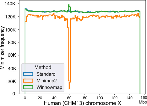
Step histogram plot showing frequency of minimizers sampled using a complete human chromosome X as the reference. Frequency of minimizers was computed in each consecutive ‘super-window’ of length 1 Mbp across the reference sequence. We compare three sampling algorithms using window length parameter w = 10. ‘Standard’ method refers to the classic minimizer sampling algorithm from Roberts et al. (2004), without any masking or modification. Minimap2 uses the standard algorithm, but masks the most frequently occurring minimizers (top 0.02%) in the reference (count $\ge 160$ for this reference). Winnowmap uses weighted minimizer sampling. Both ‘Standard’ and Winnowmap methods maintain at least one minimizer per window in their index and achieve near-uniform density. The masking heuristic in Minimap2 reduces minimizer density throughout the chromosome X, and a significant drop is observed in its long repetitive centromere (58–61 Mbp). Interestingly, we also observe a slight increase in Winnowmap’s minimizer density in this region

5.3 Benefit of weighted minimizer sampling and robust winnowing

Weighted minimizer sampling in Winnowmap includes two key optimizations, (i) robust winnowing and (ii) weighted sampling. These two optimizations are independent of one another and we evaluated the advantages of each. To do this, we compared (i) Winnowmap, (ii) a version of Winnowmap that implements only robust winnowing and (iii) a version of Minimap2 that implements the standard minimizer sampling without the masking heuristic. Accordingly, these three methods are referred to as ‘Optimization 1 + 2’, ‘Optimization 1’, and ‘Standard’, respectively, in Figure 5. As there is no masking involved, these three methods index all minimizers irrespective of their frequency. Here, we show mapping time and peak memory usage using datasets D1-D3 while keeping window length equal. We used a window length of 10 for datasets D1 and D2, and 50 for dataset D3. The ‘Standard’ method crashed on dataset D3 with a window length of 10. These results demonstrate that these Winnowmap optimizations are crucial for speed and memory efficiency.

Fig. 5.

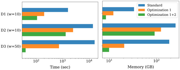
Benefit of the proposed minimizer sampling optimizations to long read mapping performance. We compare three methods: ‘Standard’ (default minimizer sampling, no masking), ‘Optimization 1’ (robust winnowing) and ‘Optimization 1 + 2’ (robust winnowing and weighted minimizer sampling). All three methods select at least one minimizer in each window. The left plot indicates total mapping time whereas the right plot indicates total memory usage, using datasets D1st. The x-axis is log-scaled in both plots. The combination of both optimizations is crucial in Winnowmap to achieve good efficiency

6 Conclusions

Minimizer sampling is a simple yet powerful technique to speed up genome sequence analysis. When this technique is used for seeding sequence alignments, minimizers with high frequency often lead to too many false-positive seed matches. The large number of false hits naturally leads to high memory-usage and runtime. To date, a popular way to deal with this issue has been to mask highly repetitive minimizers. While this masking heuristic eliminates false hits, the underlying guarantee of a minimizer seed match is lost in the process. As a result, masking decreases mapping accuracy within long genomic repeats. In this article, we describe optimizations to the standard minimizer sampling procedure and evaluate the improvements to long-read mapping. We have introduced weighted minimizer sampling, where users can specify which k-mers should be more (or less) likely to be selected as minimizers. Finally, when there are multiple equally minimum k-mers in a window (e.g. in low complexity regions), robust winnowing is effective in preventing oversampling.

We implemented weighted minimizer sampling and robust winnowing in Winnowmap. Winnowmap makes it feasible to map PacBio or ONT reads without the need for a masking heuristic. As a result, it achieves superior mapping accuracy by maintaining a uniform sampling density across the reference sequence using a simple weighting criteria.

Future work will be focused in three directions. First, we will explore more sophisticated weight functions, e.g. down-weighting erroneous k-mers in addition to repetitive k-mers. A set of likely erroneous k-mers could be detected prior to mapping by intersecting the k-mer sets of the reads and the reference genome. Second, we will test the idea of weighted minimizer sampling in other applications such as long-read overlapping and metagenomic read classification. Third, the density bounds that were discussed in this article are defined for arbitrary weights. However, in most applications, we can assume weight values are bounded between $[1/c,c]$, where c is a constant. It will be useful to derive tight bounds on the expected density under this constraint.

Funding

This research was supported in part by the Intramural Research Program of the National Human Genome Research Institute, National Institutes of Health.

Conflict of Interest: none declared.

References

- Altschul S.F. et al. (1997) Gapped BLAST and PSI-BLAST: a new generation of protein database search programs. Nucleic Acids Res., 25, 3389–3402. [DOI] [PMC free article] [PubMed] [Google Scholar]
- Baharav,T.Z. et al. (2020) Spectral Jaccard Similarity: A new approach to estimating pairwise sequence alignments. bioRxiv. doi: 10.1101/800581. [DOI] [PMC free article] [PubMed] [Google Scholar]
- Berlin K. et al. (2015) Assembling large genomes with single-molecule sequencing and locality-sensitive hashing. Nat. Biotechnol., 33, 623–630. [DOI] [PubMed] [Google Scholar]
- Broder A.Z. (1997) On the resemblance and containment of documents. In Proceedings Compression and Complexity of Sequences 1997 (Cat. No. 97TB100171), pp. 21–29. IEEE.
- Chikhi R. et al. (2015) On the representation of de Bruijn graphs. J. Comput. Biol., 22, 336–352. [DOI] [PubMed] [Google Scholar]
- Chin C.-S., Khalak A. (2019) Human genome assembly in 100 minutes. bioRxiv.
- Chum O. et al. (2008) Near duplicate image detection: min-Hash and tf-idf weighting. BMVC, 810, 812–815. [Google Scholar]
- DeBlasio D. et al. (2019) Practical universal k-mer sets for minimizer schemes. In: Proceedings of the 10th ACM International Conference on Bioinformatics, Computational Biology and Health Informatics, pp. 167–176.
- Dilthey A.T. et al. (2019) Strain-level metagenomic assignment and compositional estimation for long reads with metamaps. Nat. Commun., 10, 1–12. [DOI] [PMC free article] [PubMed] [Google Scholar]
- Frith M.C. (2011) Gentle masking of low-complexity sequences improves homology search. PLoS One, 6, e28819. [DOI] [PMC free article] [PubMed] [Google Scholar]
- Jain C. et al. (2018) A fast approximate algorithm for mapping long reads to large reference databases. J. Comput. Biol., 25, 766–779. [DOI] [PMC free article] [PubMed] [Google Scholar]
- Koren S. et al. (2017) Canu: scalable and accurate long-read assembly via adaptive k-mer weighting and repeat separation. Genome Res., 27, 722–736. [DOI] [PMC free article] [PubMed] [Google Scholar]
- Kundu R. et al. (2019) Hypo: super fast & accurate polisher for long read genome assemblies. bioRxiv.
- Kurtz S. et al. (2004) Versatile and open software for comparing large genomes. Genome Biol., 5, R12. [DOI] [PMC free article] [PubMed] [Google Scholar]
- Langmead B., Salzberg S.L. (2012) Fast gapped-read alignment with bowtie 2. Nat. Methods, 9, 357–359. [DOI] [PMC free article] [PubMed] [Google Scholar]
- Li H. (2016) Minimap and miniasm: fast mapping and de novo assembly for noisy long sequences. Bioinformatics, 32, 2103–2110. [DOI] [PMC free article] [PubMed] [Google Scholar]
- Li H. (2018. a) Evaluating Mapping Accuracy with Simulated Reads https://bit.ly/paftools (26 March 2020, date last accessed).
- Li H. (2018. b) Minimap2: pairwise alignment for nucleotide sequences. Bioinformatics, 34, 3094–3100. [DOI] [PMC free article] [PubMed] [Google Scholar]
- Marçais G. et al. (2017) Improving the performance of minimizers and winnowing schemes. Bioinformatics, 33, i110–i117. [DOI] [PMC free article] [PubMed] [Google Scholar]
- Marçais G. et al. (2018) Asymptotically optimal minimizers schemes. Bioinformatics, 34, i13–i22. [DOI] [PMC free article] [PubMed] [Google Scholar]
- Marçais G. et al. (2019) Sketching and sublinear data structures in genomics. Annu. Rev. Biomed. Data Sci., 2, 93–118. [Google Scholar]
- Miga K.H. et al. (2019) Telomere-to-telomere assembly of a complete human X chromosome. BioRxiv, 735928. [DOI] [PMC free article] [PubMed]
- Ondov B.D. et al. (2016) Mash: fast genome and metagenome distance estimation using minhash. Genome Biol., 17, 132. [DOI] [PMC free article] [PubMed] [Google Scholar]
- Ono Y. et al. (2013) PBSIM: PacBio reads simulator-toward accurate genome assembly. Bioinformatics, 29, 119–121. [DOI] [PubMed] [Google Scholar]
- Orenstein Y. et al. (2016) Compact universal k-mer hitting sets In International Workshop on Algorithms in Bioinformatics. Springer, pp. 257–268. [Google Scholar]
- Popic V., Batzoglou S. (2017) A hybrid cloud read aligner based on minhash and kmer voting that preserves privacy. Nat. Commun., 8, 15311. [DOI] [PMC free article] [PubMed] [Google Scholar]
- Rhie A. et al. (2020) Merqury: reference-free quality and phasing assessment for genome assemblies. bioRxiv. [DOI] [PMC free article] [PubMed]
- Roberts M. et al. (2004) Reducing storage requirements for biological sequence comparison. Bioinformatics, 20, 3363–3369. [DOI] [PubMed] [Google Scholar]
- Rowe W.P. (2019) When the levee breaks: a practical guide to sketching algorithms for processing the flood of genomic data. Genome Biol., 20, 199. [DOI] [PMC free article] [PubMed] [Google Scholar]
- Sahlin K., Medvedev P. (2020) De novo clustering of long-read transcriptome data using a greedy, quality-value based algorithm. J. Comput. Biol., 27, 472–484. [DOI] [PMC free article] [PubMed] [Google Scholar]
- Sahlin K. et al. (2020) Error correction enables use of oxford nanopore technology for reference-free transcriptome analysis. bioRxiv. [DOI] [PMC free article] [PubMed]
- Schleimer S. et al. (2003) Winnowing: local algorithms for document fingerprinting. In Proceedings of the 2003 ACM SIGMOD International Conference on Management of Data, pp. 76–85. ACM.
- Schneider V.A. et al. (2017) Evaluation of GRCh38 and de novo haploid genome assemblies demonstrates the enduring quality of the reference assembly. Genome Res., 27, 849–864. [DOI] [PMC free article] [PubMed] [Google Scholar]
- Shafin K. et al. (2020) Nanopore sequencing and the Shasta toolkit enable efficient de novo assembly of eleven human genomes. Nat. Biotechnol., 1–10. [DOI] [PMC free article] [PubMed]
- Smith K.C. (2011) Sliding Window Minimum Implementations https://goo.gl/8RC54b (16 January 2020, date last accessed).
- Smith T.F., Waterman M.S. (1981) Identification of common molecular subsequences. J. Mol. Biol., 147, 195–197. [DOI] [PubMed] [Google Scholar]
- Xin H. (2018) Methods for reducing unnecessary computation on false mappings in read mapping. Ph.D. thesis.
- Yu Y.W. et al. (2015) Entropy-scaling search of massive biological data. Cell Syst., 1, 130–140. [DOI] [PMC free article] [PubMed] [Google Scholar]