SMAP L-Band Microwave Radiometer: Instrument Design and First Year on Orbit

Abstract

The Soil Moisture Active–Passive (SMAP) L-band microwave radiometer is a conical scanning instrument designed to measure soil moisture with 4% volumetric accuracy at 40-km spatial resolution. SMAP is NASA’s first Earth Systematic Mission developed in response to its first Earth science decadal survey. Here, the design is reviewed and the results of its first year on orbit are presented. Unique features of the radiometer include a large 6-m rotating reflector, fully polarimetric radiometer receiver with internal calibration, and radio-frequency interference detection and filtering hardware. The radiometer electronics are thermally controlled to achieve good radiometric stability. Analyses of on-orbit results indicate that the electrical and thermal characteristics of the electronics and internal calibration sources are very stable and promote excellent gain stability. Radiometer NEDT < 1 K for 17-ms samples. The gain spectrum exhibits low noise at frequencies >1 MHz and 1/f noise rising at longer time scales fully captured by the internal calibration scheme. Results from sky observations and global swath imagery of all four Stokes antenna temperatures indicate that the instrument is operating as expected.

I. Introduction

THE National Aeronautics and Space Administration’s (NASA’s) Soil Moisture Active–Passive (SMAP) satellite was launched into a 685-km near sun-synchronous 6A.M./P.M. orbit on January 31, 2015. SMAP’s L-band microwave radiometer was commissioned in February and March and has now reached its milestone of one year of successful operation. A 3-D rendering of the SMAP observatory in its fully deployed configuration is shown in Fig. 1. SMAP is the third in a series of modern L-band radiometers after the European Space Agency’s Soil Moisture Ocean Salinity (SMOS) satellite launched in 2009 and NASA’s Aquarius instrument aboard Argentina’s Comisión Nacional de Actividades Espaciales Satelite de Aplicaciones Cientificas (SAC)-D satellite launched in 2011 [1]–[3]. SMAP’s primary science objective is to provide soil moisture measurements with an uncertainty < 0.04 m³m⁻³ for terrain having vegetation water contents up to 5 kg/m². For the radiometer, this objective requires radiometric uncertainty <1.3 K (with fore and aft averaging) with <40-km spatial resolution.

Fig. 1.

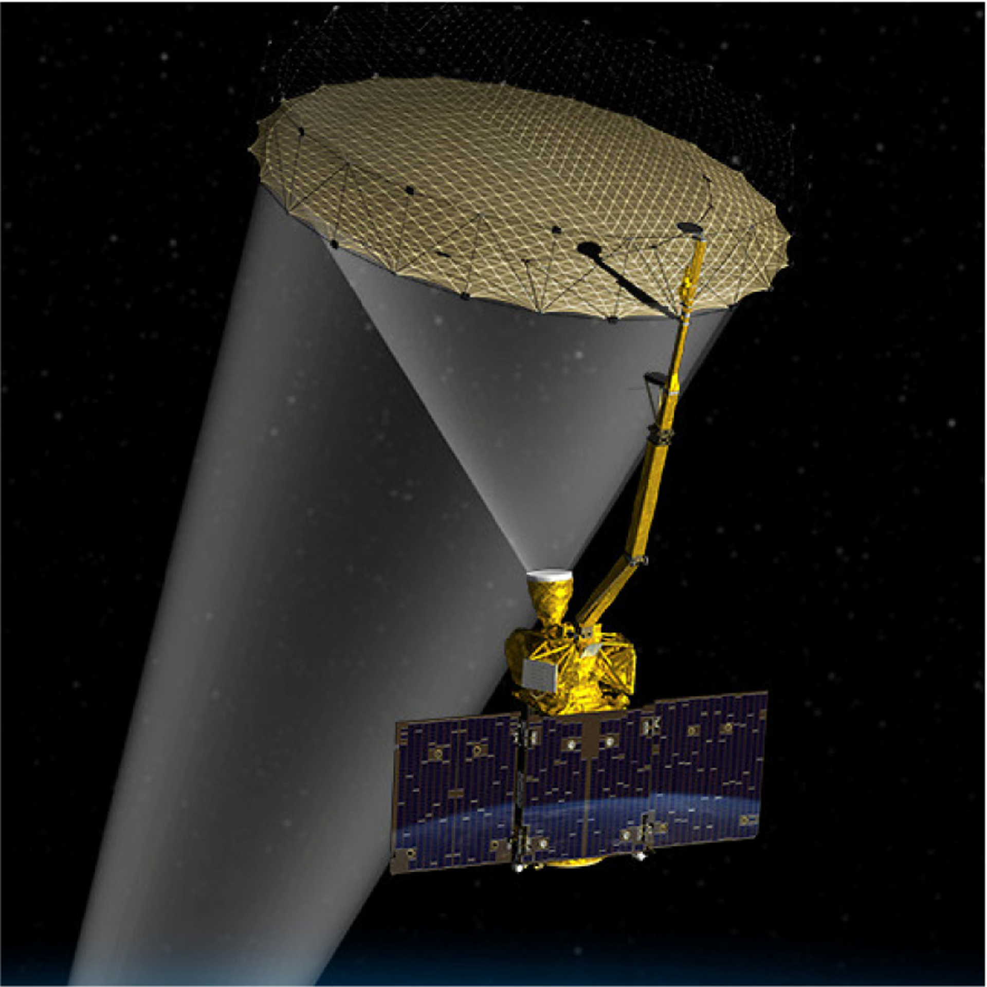
SMAP observatory in fully deployed configuration. Image credit: NASA/JPL-Caltech.

SMAP is NASA’s first Earth Systematic Mission developed in response to its first Earth science decadal survey [4]. The SMAP mission high-level science requirements and derived instrument requirements related to the radiometer are shown in Table I (adapted from [5]). Early in its mission, SMAP provided 10-km resolution soil moisture globally every three days using a combined active–passive microwave instrument. The instrument comprises a radiometer and a synthetic aperture radar (SAR), which both share a single antenna. In July, the radar ceased transmissions and has remained in the receive-only mode since [6]. By itself, the radiometer enables 40-km resolution soil moisture with the same three-day global coverage. Nonetheless, with its conical-scanning (real aperture) antenna and advanced radio-frequency interference (RFI) mitigation capabilities, the SMAP radiometer is providing high-quality brightness temperature measurements of Earth’s land, ice, and ocean surfaces.

TABLE I.

SMAP Radiometer Science and Instrument Requirements

Scientific Requirements	Measurement	Instrument Requirements	Functional
Soil Moisture: 0.04 m3m−3 volumetric uncertainty (1-σ) in the top 5 cm for vegetation water content ≤ 5 kg m−2; Hydroclimatology at 40-km resolution		L-Band Radiometer (1.41 GHz): Polarization: V, H, T3 and T4 Project 3-dB beamwidth ≤ 40 km Radiometric Uncertainty ≤ 1.3 K Constant 40° incidence angle
Sample diurnal cycle at consistent time of day (6am/6pm Equator crossing); Global, 3-day (or better) revisit		Swath Width: 1000 km Minimize Faraday rotation
Observation over minimum of three annual cycles		Baseline three-year mission life

Observation over minimum of Baseline three-year mission life three annual cycles

The two key technology innovations—the large scanning 6-m reflector and the total power radiometer receiver with advanced RFI detection and filtering capabilities—combined make the SMAP radiometer unique. On-orbit results of SMAP’s RFI mitigation capabilities are discussed in [7]. In other ways, the SMAP radiometer derives its requirements and/or design from past radiometer systems. The front-end architecture with a 6-m antenna shared with the radar was inherited from the preliminary design of the Hydrosphere State (Hydros) Earth System Science Pathfinder (ESSP) mission, which was selected as an alternate ESSP by NASA but did not proceed with development in 2005 [5]. SMAP’s antenna is conical scanning with a full 360° field of regard. However, there are several key differences (some unique) from previous low-frequency conical scanning radiometers like WindSat or Advanced Microwave Scanning Radiometer for the Earth Observing System [8], [9]. Most obvious is the lack of external warm-load and cold-space reflector, which normally provides radiometric calibration through the feed horn. Rather, SMAP’s internal calibration scheme is based on the Jason Microwave Radiometer, the Aquarius push broom radiometers, and the SMOS radiometer using reference load switches and coupled noise diodes [9]–[11]. Switching of the internal calibrations sources is synchronized with the radar operation, as it is on Aquarius, so the radiometer oversamples the footprint. Both SMAP and Aquarius utilize this oversampling technique for time-domain detection and filtering of radio-frequency interference [12], [13]. Like WindSat, SMAP measures all four Stokes parameters with fore and aft viewing; unlike WindSat, SMAP uses coherent detection for the third and fourth Stokes parameters implemented in a digital receiver back end for the first time in space in a conical scanning radiometer [14]. The first two modified Stokes parameters, T_V and T_H, are the primary science channels used by the soil moisture retrieval algorithm [15]. The T₃ channel measurement provides correction of Faraday rotation caused by the ionosphere [16]. The T₄ channel is measured as a consequence of the receiver design and the data are used to detect RFI. The most significant difference SMAP has from all past spaceborne radiometer systems is its aggressive hardware and algorithm approach to RFI detection and filtering [7], [13]. The requirement to detect and filter RFI drives and exploits features of the SMAP design.

Here, the main features of the SMAP radiometer design, results of early orbit operations, and observations for the first year up through March 2016 are presented. Section II covers the observatory, swath, and antenna design. Section III describes the radiometer electronics and their calibration before launch. Activities and results of prelaunch calibration and early operations on-orbit are discussed in Sections IV and V. A review of one year of data is discussed in Sections VI and VII.

II. Observatory and Antenna Design

SMAP orbits Earth at 685-km altitude with the spacecraft pointing to geodetic nadir. The instrument antenna points 35.5° away from nadir and generates a 2.4° 3-dB beamwidth for the radiometer. This geometry creates an instantaneous field-of-view (IFOV) of 36-by-47 km with an Earth incidence angle of 40°. The distance across the swath is 1000 km from IFOV center to center. This swath width, combined with the orbit parameters, allows the whole of Earth’s surface to be covered in three days (except for typical pole holes) with no gaps at the equator.

Imaging is accomplished by conical scanning the antenna beam with a full 360° field of regard. The antenna rotates at 14.6 r/min, completing a scan with 3200-km circumference every 4.1 s. Along-scan averaging occurs over 14 ms, which smears the beam along scan to create a 39 × 47 km effective field of view. Along-scan sampling occurs every 11 km, which is faster than the 20-km Nyquist criterion. With the spacecraft moving at 6.8 km/s speed over ground, the along track (or across scan) sampling at center of swath is 28 km—slightly slower than the 24-km Nyquist criterion. The spatial sampling geometry near the center of swath is shown in Fig. 2.

Fig. 2.

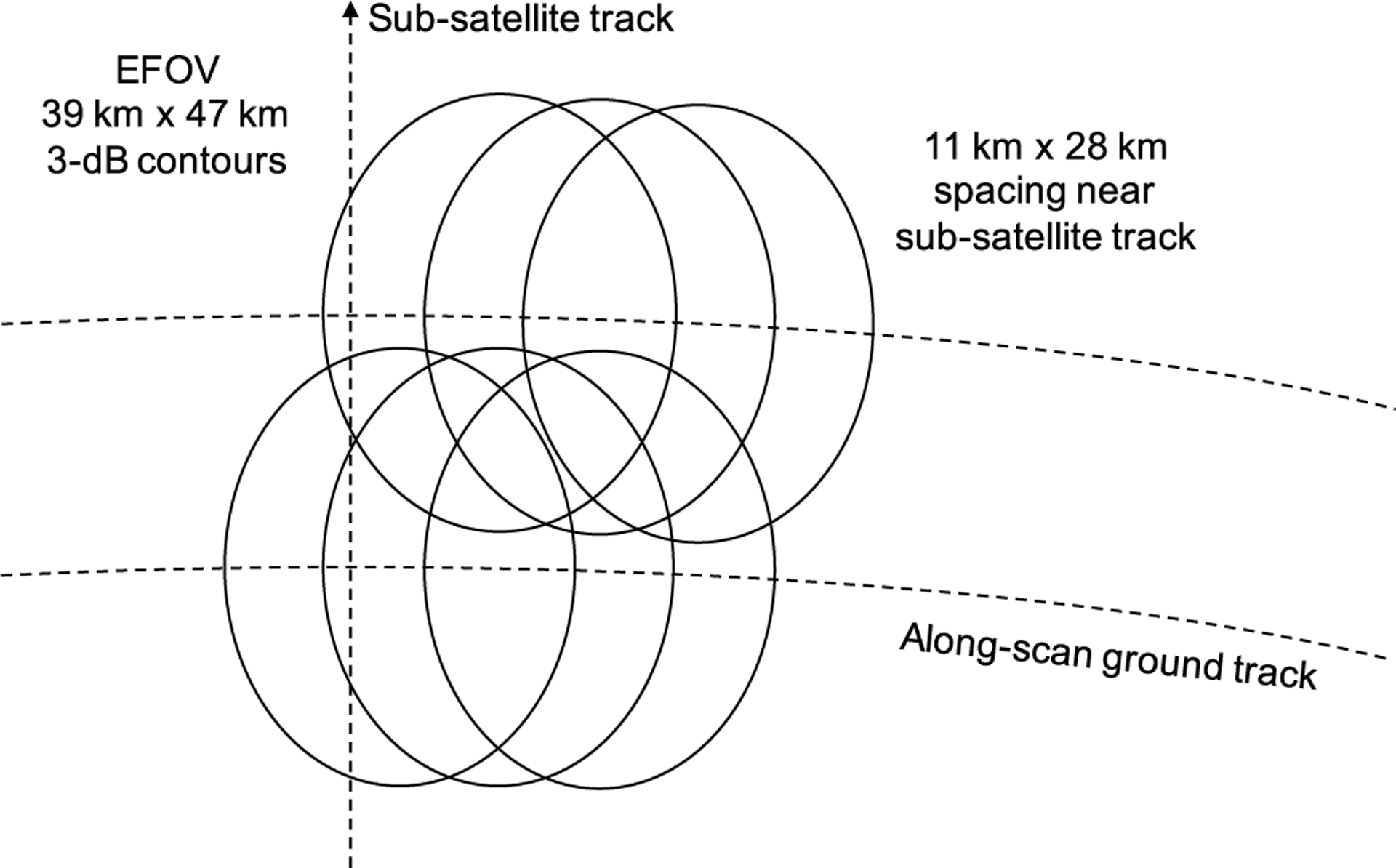
Footprint spacing near subsatellite track.

The instrument antenna, shared between the radiometer and the SAR, is composed of a 6-m offset reflector fed by a dual polarized, dual-band feed-horn. With a focal length of 4.2 m and a projected diameter of 6 m, a Kevlar net shapes the deployable mesh reflector into a triangularly faceted surface with an rms error compared with a perfect paraboloid less than 2 mm or about 1% wavelength. Optimized for both the radiometer (1.4015–1.4255 GHz) and the SAR (1.2168–1.2982 GHz) frequency bands, the feed-horn includes an ortho-mode-transducer (OMT) to separate horizontal and vertical polarizations. The OMT is partly made of titanium to thermally isolate the horn, which is exposed to the thermal radiation environment, from the radiometer electronics.

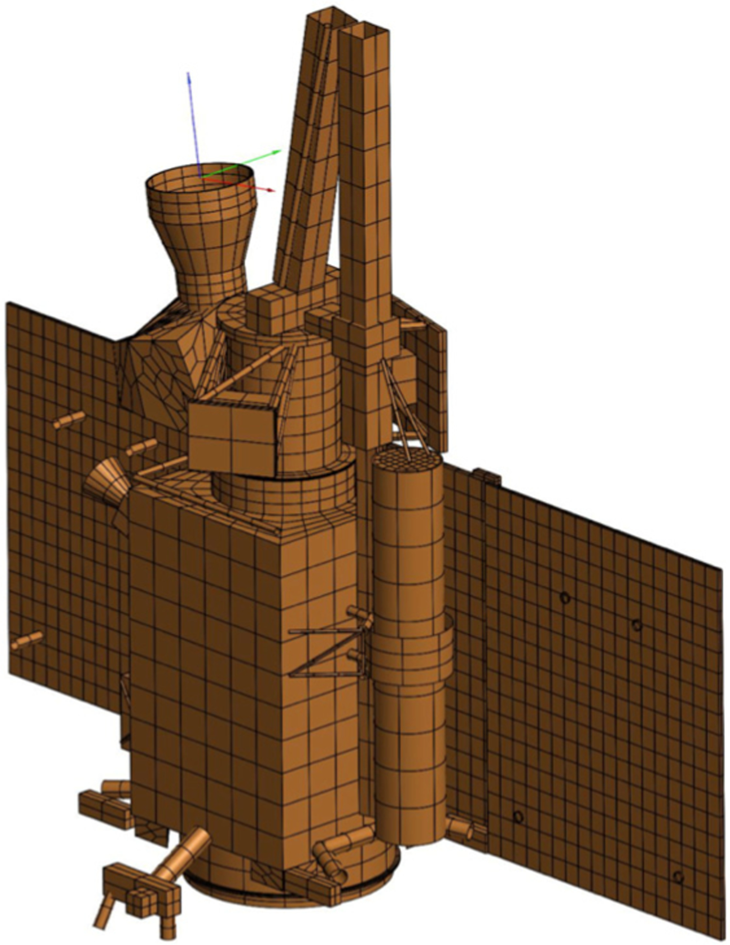
Fig. 3 shows a comparison between the computer-aided drawing model of the SMAP observatory with the reflector fully deployed and its RF model used to predict the antenna performance. All significant details relative to 21-cm wavelength were included into the model to get the best possible accuracy in the radiation pattern. The reflector antenna radiation pattern was not measured before launch; therefore, a very accurate antenna pattern knowledge was required to verify performance requirements (e.g., beam efficiency) and for the initial radiometer calibration. A 1/10th scale model replicating all major aspects of the flight hardware was also designed, built, and tested to validate the RF model. Final requirement verification was then done with a combination of flight feed assembly measurements, scale model predictions, and measurements and flight model predictions. A horizontal polarization pattern cut along the along-scan direction (horizontal direction) is shown in Fig. 4. The main lobe has a half-power beamwidth of 2.4°. The backlobes, primarily due to feed pattern spillover and edge diffraction, fall into the space region. The beam efficiency for vertical and horizontal polarizations is 88%, with most of the nonmain lobe contribution directed toward space.

Fig. 3.

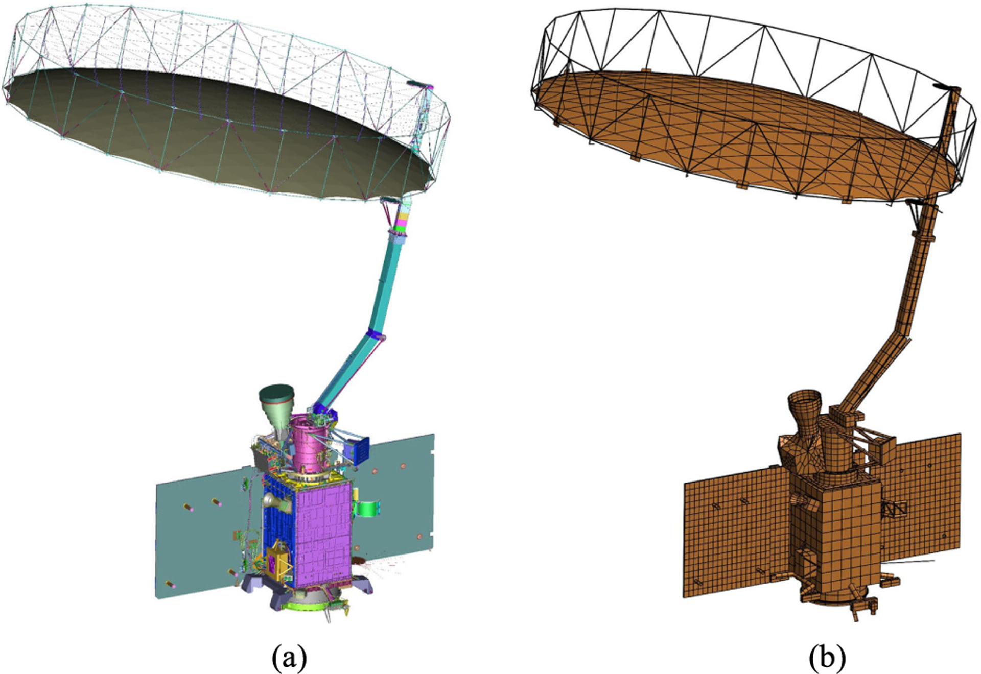
SMAP observatory. (a) Solid model from mechanical design software. (b) Mesh model for the 3-D antenna analysis software.

Fig. 4.

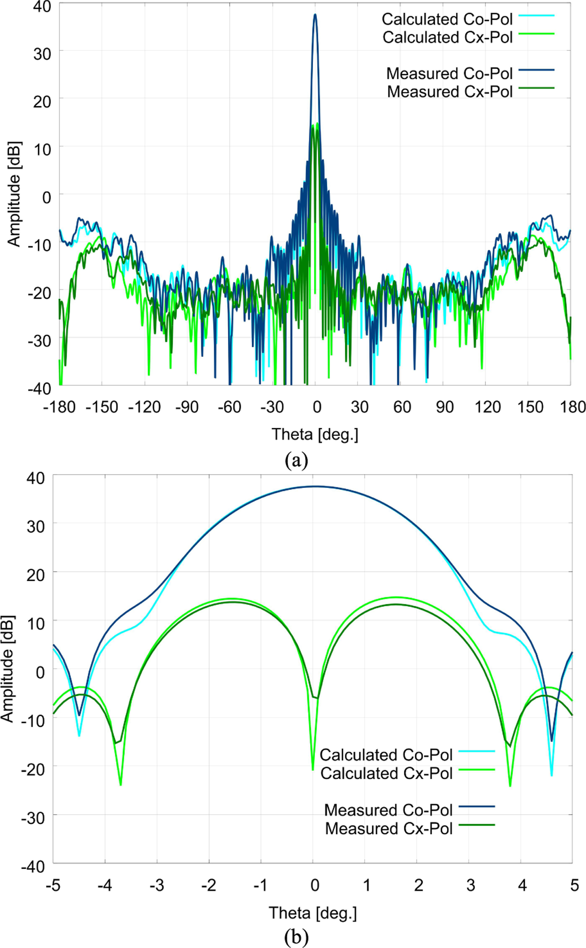
Antenna pattern cut of horizontal polarization along the antenna scanning direction for (a) full pattern and (b) main lobe. Comparison is between calculated and measured data for the 1/10 SMAP scale model.

III. Radiometer Electronics Design

The radiometer electronics consist of antenna feed network, radiometer front end (RFE), radiometer back end (RBE), and radiometer digital electronics (RDE). These subsystems are shown in Fig. 5 with signal flow from right to left. The antenna feed network includes an external noise source and diplexers to separate radar frequencies from the radiometer path. The external noise source signal is added to the antenna signal, but is not used as a primary calibration source and is present for redundancy. The diplexers include additional filtering to limit the amount of RFI entering the RFE. The RFE contains the primary internal calibration switches and noise source, RF amplification, and additional filtering. The internal noise source signal is added to the reference signals to provide RFI-free gain calibration. The RBE downconverts the RF signals to a lower IF frequency using a common phase-locked local oscillator (PLO). The reference clock for the PLO also clocks the analog-to-digital converters (ADCs) in the RDE. The ADCs sample and quantize the IF signals for processing by a field programmable gate array-based digital signal processor (DSP). The DSP generates detected power for the full passband (fullband data) and for 16 channels spaced evenly across the passband (subband data). The RDE generates timing signals needed to control the internal calibration sources and synchronizes radiometer integration with the radar timing. Finally, data are packetized by the RDE and sent to spacecraft mass storage for later downlink to the ground.

Fig. 5.

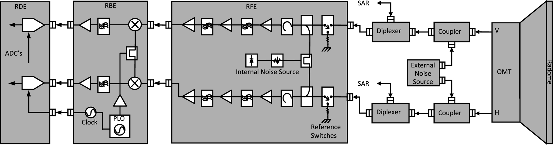
Radiometer block diagram including feed network, radiometer front end, radiometer back end, and digital electronics. Signal flow is from right to left.

The RF system is designed to make linear radiometric measurements in the presence of RFI up to an interference-to-noise ratio of 6 dB or an effective added noise temperature of 2000 K due to RFI out of a typical 500 K system temperature. Above 2000 K, the accumulators in the integrator logic saturate. Cascaded filtering and amplification sufficient to operate each stage at a maximum power of 24-dB below 1-dB compression keeps the error contribution from nonlinearity due to RFI signals negligible over this range. The total system frequency response is shown in Fig. 6. Note that the response is 30 dB below peak at the allocation edges at 1400 and 1427 MHz. The rolloff to >100 dB is much faster on the low side because of the presence of air search radars and less stringent on the high side because of fewer known RFI sources.

Fig. 6.

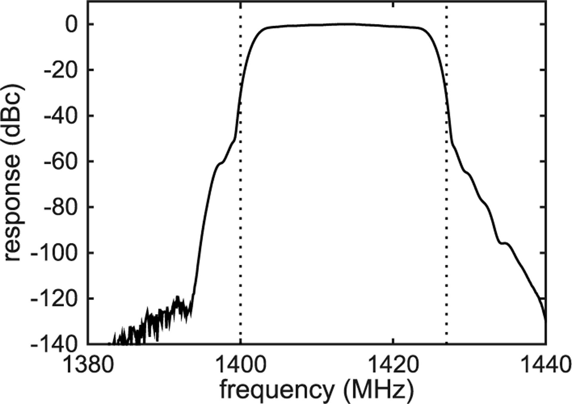
Frequency response of SMAP microwave radiometer. This response combines RF, IF, and digital filters. Vertical dotted lines: spectrum allocation at 1400–1427 MHz.

The digital back end replaces conventional diode detectors with moment accumulators and complex cross-correlators. The first four moments of the ADC outputs are estimated by the RDE. The science-processing algorithm computes the second central moment using the first and second moments to estimate the total power [17]. These data are used to estimate antenna temperature. The kurtosis (used by the RFI detectors) is computed in a similar manner using raw moments. The complex cross-correlation coefficient is also measured by the RDE and is used in the science-processing algorithm to estimate third and fourth Stokes parameters.

Third and fourth Stokes parameters are measured by the radiometer to compensate for Faraday polarization basis rotation caused by the ionosphere and to be used as RFI detectors. The driving requirement on the receiver was to minimize (relative to 24-MHz bandwidth) the differential group delay between the vertical and horizontal channels. Because the complex correlation is measured, any mean phase difference between vertical and horizontal polarizations can be compensated by a complex coefficient multiplication in the science-processing algorithm. Phase slope difference, however, would attenuate the correlation between signals, and is minimized in the design by using symmetry and avoiding unnecessarily long cables of different lengths.

The radiometer integrator logic operates synchronously with the radar, whereby the radiometer integrates received power during the radar receive window and blanks during the transmit window. Timing is shown in Fig. 7. The fundamental unit of integration is 300 μs contained within a pulse-repetition interval (PRI). Fullband data are integrated at this rate. Subband data, however, are integrated 1.2 ms over a packet defined as four PRI’s. During a footprint, eight packets are utilized to view the Earth for 9.6 ms and four packets to view the internal reference load and noise source or calibration for 4.8 ms. Because of a small amount of blanking during radar transmit and calibration switching setup time, this cycle occurs on a 17 ms period.

Fig. 7.

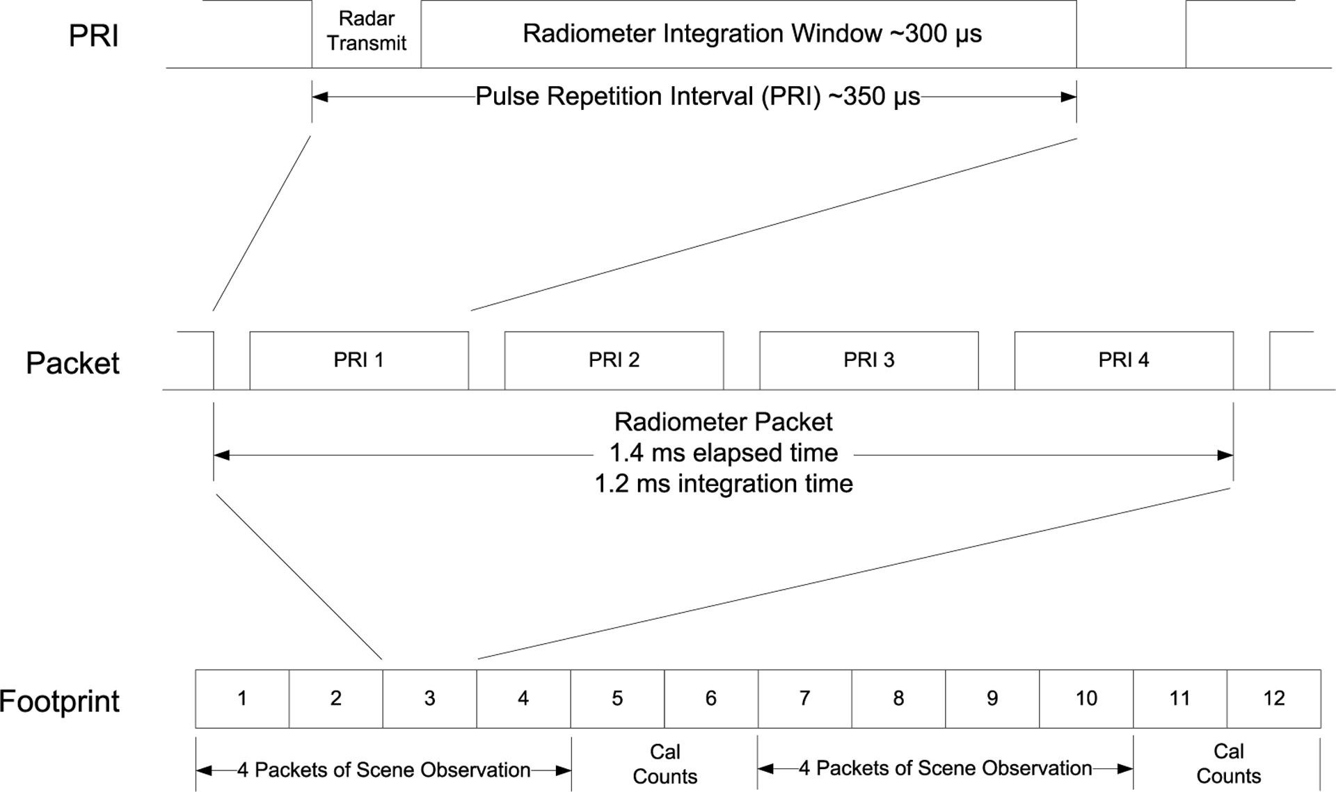
Timing of radiometer sampling for a PRI, a packet, and a footprint.

The radiometer timing, antenna beamwidth and scan rate, and ground software averaging are coordinated, and so the equivalent low-pass processes work together to produce Nyquist sampled footprints along the scan direction. The frequency responses of the processes are shown in Fig. 8. The on-board integrators are represented by the two rightmost traces (dashed-dotted and dashed lines) for 1 and 4 PRI’s, respectively. The eight-packet (32-PRI) integration done in the ground software to form a footprint has a low-pass response indicated by a solid trace labeled L1B_TB. The Level 1 product footprint process has a 3-dB point at 30 Hz, which fully samples the low-pass process created by the antenna pattern sweeping across the Earth. The bump in the footprint response near 100 Hz is caused by the interleaving of antenna looks with calibration looks, which robs integration time from the scene. A balance is struck in the algorithm design between increased NEDT versus decreased ΔG/G noise. The high-frequency energy at 100 Hz in the antenna averaging response is merely white noise aliased into the footprints and equivalent to the increase in NEDT due to limiting antenna integration time. Finally, the dotted line marked “antenna” shows the equivalent low-pass response of the antenna approximated by a Gaussian beam (sweeping along-scan in azimuth at 770 km/s speed over ground) to naturally occurring thermal radiation.

Fig. 8.

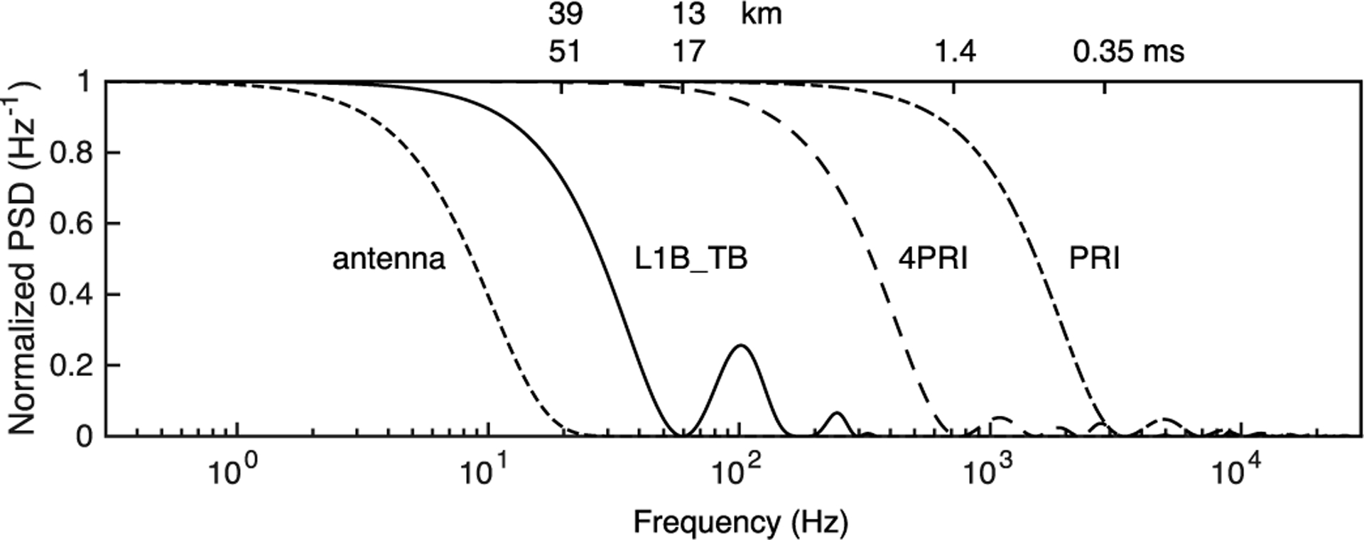
Representative frequency response of averaging performed in radiometer operation and processing. The two rightmost traces (dashed-dotted and dashed lines) show the low-pass response of the on-board boxcar integrator over one and four PRIs, respectively. The solid trace shows the frequency response of the calibrated antenna temperatures found in the Level 1B_TB data product. Finally, the dotted line marked “antenna” shows the equivalent low-pass response of the antenna beam (sweeping along-scan in azimuth) to naturally occurring thermal radiation.

The four packets of calibration observations are partitioned into two packets for reference load and two packets for reference plus noise diode. Conventionally, noise is injected prior to a reference switch; however, on SMAP as on Aquarius, RFI is such a concern that the noise injection is done behind the switch to ensure that the radiometer can be calibrated regardless of RFI entering the antenna. The noise source on SMAP, unlike Aquarius, is a single noise source split coherently between the vertical and horizontal receiver channels. This method was chosen, because the digital receiver has negligible cross-polarization coupling and the total power and cross-correlation detectors can be calibrated essentially independently. The phase of the correlated noise source was set to 40^o to enable calibration of the real and imaginary outputs of the correlator using the same calibration state.

The radiometer science-processing algorithm uses these pairs of reference and noise diode counts to compute gain and offset coefficients, which are then further averaged over a longer time period (multiple footprints) to reduce estimation noise. The gain and offset are computed twice per footprint in the science-processing algorithm and then averaged with a 5000-tap, uniform, centered noncausal filter. The frequency responses of these filters are discussed in the on-orbit data section below. Careful attention was paid to thermal control to allow gain and offset coefficient averaging over 10s of seconds and to help maintain radiometer stability on orbital and seasonal time scales. The combination of passive thermal design with an active proportional controller achieves 0.1 ^oC/orbit within the RFE [22], [23]. Worst-case orbital results are also discussed in the on-orbit results section below.

IV. Prelaunch Calibration

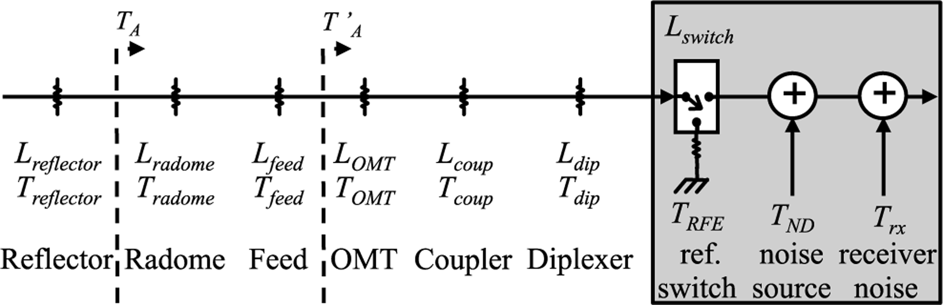
The prelaunch calibration of the radiometer includes both a radiometric and a polarimetric exercise to characterize temperature dependence of the reference and noise source looks and receiver phase imbalance relative to the feedhorn input. The radiometric calibration was accomplished using techniques similar to [18] and polarimetric calibration [19]. The goal of the radiometric calibration is to characterize the losses (or equivalent) and noise diode added noise temperature, represented by the simplified loss model shown in Fig. 9, for use in the science-processing algorithm. Likewise, the goal of the polarimetric calibration is to determine the polarimetric efficiency and phase differences of the receiver channels.

Fig. 9.

Simplified calibration model showing lumped losses and physical temperatures.

In the science-processing algorithm, the antenna temperature referenced to the feedhorn output/OMT input is computed from radiometer output counts using a two-point calibration model

$$T_A^{\prime }=T_{\text{ref}}^{\prime }-\frac{c_{\text{ref}}-c_A}{c_{\text{ND},R}-c_{\text{ref}}}{T}_{\text{ND}}^{\prime }$$ (1)

where T′_ref is the internal reference load noise temperature and T′_ND the coupled noise source temperature referred to the feedhorn output/OMT input. The radiometer output counts are represented by c_x, where x indicates reference (ref), antenna (A), and noise diode + reference (ND, R) states. The intermediate antenna temperature (1) is input-referred to the feedhorn aperture by correcting for feed and radome losses and physical temperatures

$$T_A=L_{\text{radome }}{L}_{\text{feed }}{T}^{\prime }A-L_{\text{radome}}\left(L_{\text{feed }}-1\right)T_{\text{feed }}-\left(L_{\text{radome }}-1\right)T_{\text{radome }}$$ (2)

where L_x and T_x are the loss factors and physical temperatures for xequal to the radome and feed. The internal calibration temperatures can be expressed as functions of the lumped losses and physical temperatures shown in the loss model (Fig. 9)

$${T^{\prime }}_{\text{ref}}=L_{\text{OMT}}{L}_{\text{coup}}{L}_{\text{dip}}{T}_{RFE}-L_{\text{OMT}}{L}_{\text{coup}}\left(L_{\text{dip}}-1\right)T_{\text{dip}}-L_{\text{OMT}}\left(L_{\text{coup}}-1\right)T_{\text{coup}}-\left(L_{\text{OMT}}-1\right)T_{\text{OMT}}$$ (3a)

$${T^{\prime }}_{\text{ND}}=L_{\text{OMT}}{L}_{\text{coup}}{L}_{\text{dip}}{L}_{\text{switch}}{T}_{\text{ND}}.$$ (3b)

Alternately, (3a) and (3b) can be approximated using a linear model

$${T^{\prime }}_{\text{ref}}=T_{\text{RFE}}+c_{\text{RFE},\text{ ref }}\Delta T_{\text{RFE}}+c_{\text{OMT,ref}}\Delta T_{\text{OMT}}+c_{\text{coup,ref }}\Delta T_{\text{coup }}+c_{\text{dip,ref }}\Delta T_{\text{dip }}+T_{\text{offset }}$$ (4a)

$${T^{\prime }}_{\text{ND}}=T_{\text{ND}}+c_{\text{RFE},\text{ND}}\Delta T_{\text{RFE}}+c_{\text{OMT},\text{ND}}\Delta T_{\text{OMT}}+c_{\text{coup},\text{ND}}\Delta T_{\text{coup}}+c_{\text{dip},\text{ND}}\Delta T_{\text{dip}}$$ (4b)

where coefficients c_x are derived from prelaunch thermal vacuum (TVAC) testing and ΔT_x indicates physical temperature deviation away from the reference temperature used in the linear model fitting.

The TVAC tests consisted of a series of data collections with the radiometer at different combinations of controlled temperatures for each zone. The first TVAC test was limited to the radiometer electronics and the coaxial components portion of the feed network. Each major component was installed on an individually controlled heater plate and connected together using spaceflight coaxial cables, and temperatures were then varied ±10 °C about 20 °C after [20]. A coaxial calibration source comprising a temperature stabilized matched termination and coldFET was used to provide a two-point calibration. The coldFET was calibrated against a liquid nitrogen coaxial standard load. A second TVAC test was performed with the OMT and feedhorn installed viewing a flat ferrite tile absorber plate. While data taken in the first were used to obtain the sensitivity of the coupler, diplexer, and the internal calibration sources to their physical temperature, the second test yielded the sensitivity of the calibration to OMT and feedhorn temperatures. The resulting calibration coefficients are shown in Table II. There is a relative lack of sensitivity of the reference load antenna-referred temperature due to variations in feed network components; however, the reference load temperature is quite sensitive to changes in the RFE temperature as indicated by the 20% value of c_RFE, likely due to changes in thermal gradients. The noise source has a temperature sensitivity of c_RFE/T_ND= 2.5 and 2.7 ppt/°C due to RFE temperature changes for the vertical and horizontal polarization channels, respectively.

TABLE II.

SMAP Radiometer Calibration Coefficients (Full Band)

		cRFE	cOMT	ccoup	cdip
$T_{\text{ref}}^{\prime }$	V-pol	0.205	4.78×10−5	−0.052	−0.073	Toffset = 0.225 K
	H-pol	0.208	5.23×10−5	−0.056	−0.064	Toffset = 0.741 K
$T_{\text{ND}}^{\prime }$	V-pol	1.18	0.015	0.036	0.002	TND = 465 K
	H-pol	1.24	0.012	0.053	0.048	TND = 452 K

The radiometer’s complex cross correlator is used to measure the third and fourth Stokes parameters. The radiometer has a symmetric design, but the two polarization channels are not necessarily phase balanced or spectrally balanced. A digitally controlled correlated noise source with an adjustable phase was used to determine that the polarimetric efficiency of the system was effectively unity (0.999). The two channels have the same passband response and negligible group delay difference. Nonetheless, as the received signals propagate along the receiver channels, the relative correlation angle will be changed, as the receiver’s channel phase imbalance is nonzero. Scattering parameter measurements versus temperature indicate that phase imbalance is quite stable. For example, the RFE interchannel phase imbalance varies 0.03°/°C. This amount is negligible considering the performance of the thermal control system. Thus, phases were measured at room temperature using different techniques during integration and calibration of the radiometer.

First, network analyzer measurements show the internal calibration noise diode, which is imbedded inside the RFE and has a phase imbalance (from the RFE input to output) of 1.6°. Positive sign means that the v-pol channel has longer equivalent electrical length. The path lengths between the RFE and RDE are unequal, creating an additional −41° phase shift, which was measured by a network analyzer and verified using the radiometer correlator. Finally, to calibrate the channel phase imbalances in the radiometer before the RFE inputs, a polarizing grid over LN2 calibration target was used. The principle of this test is to create linearly polarization radiation at the feedhorn input. Rotating the grid generates a third Stokes parameter with a correlation coefficient rotated by the receiver’s total phase imbalance in the complex plane. Excluding the channel phase imbalance after the RFE inputs, the channel phase imbalance from the feedhorn to the RFE inputs is 39°. These phase differences are used in the science-processing algorithm to produce the third and fourth Stokes antenna temperatures.

V. Early On-Orbit Activities

The stowed configuration of the SMAP antenna offers an unobstructed view of deep space to the feedhorn (see Fig. 10). The radiometer was powered on February 12, 2015 to take advantage of the stowed configuration. Using this well-known calibration point, one calibration parameter in the radiometer can be adjusted. The noise source was chosen, because it has the largest uncertainty remaining from prelaunch calibration testing. Estimated cold space antenna temperatures were expected to be approximately 4 ± 9 K (3-σ) based on prelaunch calibration parameters and their uncertainties. The noise source prelaunch uncertainty of 1% is largely responsible for errors in this configuration. Other error sources include internal reference load temperature, front-end component loss, and antenna feed pattern uncertainties. A typical orbit of antenna temperature measurements is shown in Fig. 11. The results based on prelaunch calibration for V-pol are 5 K too low; however, after noise source correction, the measured antenna temperature matches the expected cold-space antenna temperatures quite well. The H-pol results showed only 1 K initial discrepancy and similar agreement after correction. The radiometer was powered OFF on February 13 to prepare for reflector deployment.

Fig. 10.

Spacecraft model shows feedhorn viewing cold space with stowed reflector.

Fig. 11.

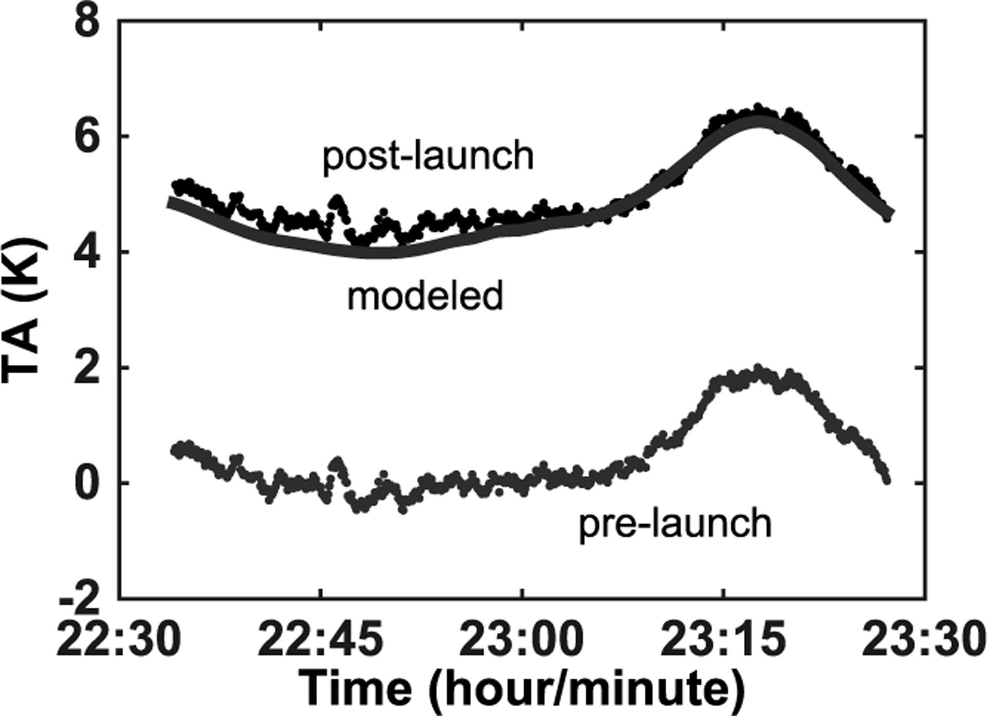
Antenna temperature (V-pol) measured in stowed configuration showing pre- and post-launch calibration results compared with modeled cold-space antenna temperature. The initial result is biased 5 K low consistent with prelaunch calibration uncertainty. H-pol measurements showed a smaller 1-K difference.

After accomplishing the space view, the reflector was deployed in a static configuration. The radiometer was powered ON again on February 27–28, 2015 to provide information to aid reflector deployment verification. The reflector was pointed aft of the spacecraft and the nadir angle was predicted to be slightly smaller than that when spinning because of boom deflection due to centrifugal force. The results of this test were favorable.

Both brightness temperature response and NEDT measurements are as expected. As shown in Fig. 12, brightness temperature response over land, ice, and ocean are reasonable (note that the color scale is limited to emphasize variations over land). High brightness temperatures are seen over rain forest in South America and West Africa and deserts in North Africa and Middle East. NEDT values estimated by the science-processing algorithm are 0.8 and 1.1 K over ocean and land, respectively. These values are consistent with instrument design specifications.

Fig. 12.

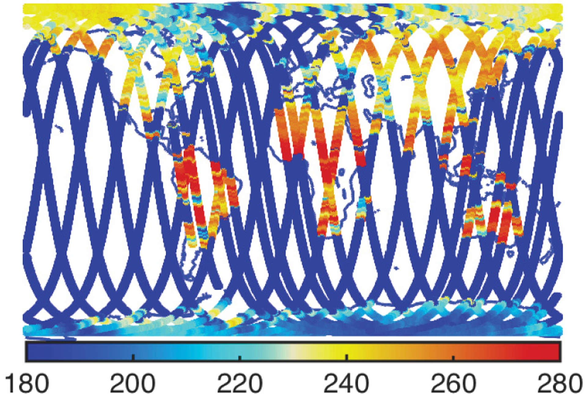
Horizontally polarized brightness temperature (K) measured with static (nonrotating) antenna. Width of the swath is 40 km and is exaggerated here for clarity.

On March 31, 2015, the radiometer reflector was rotating at operational speed and the instrument electronics were powered back on. After a check out period, the radiometer was declared operational. It has been operating successfully since.

VI. First Year on Orbit

The radiometer error budget is dominated by NEDT because of the narrow time-bandwidth product (9.6 ms by 24 MHz) available to the system. The orbit average NEDT for all four Stokes antenna temperatures is shown in Fig. 13 during the first year of operation. The orbit average NEDT is consistent with an average over land, ocean, and ice scenes and is stable throughout the year with mean value 0.90 and 0.96 K for horizontal and vertical polarizations, respectively. The NEDT for third and fourth Stokes parameters is 1.34 K, which is approximately the expected factor of √2 larger than NEDT for vertical and horizontal polarizations.

Fig. 13.

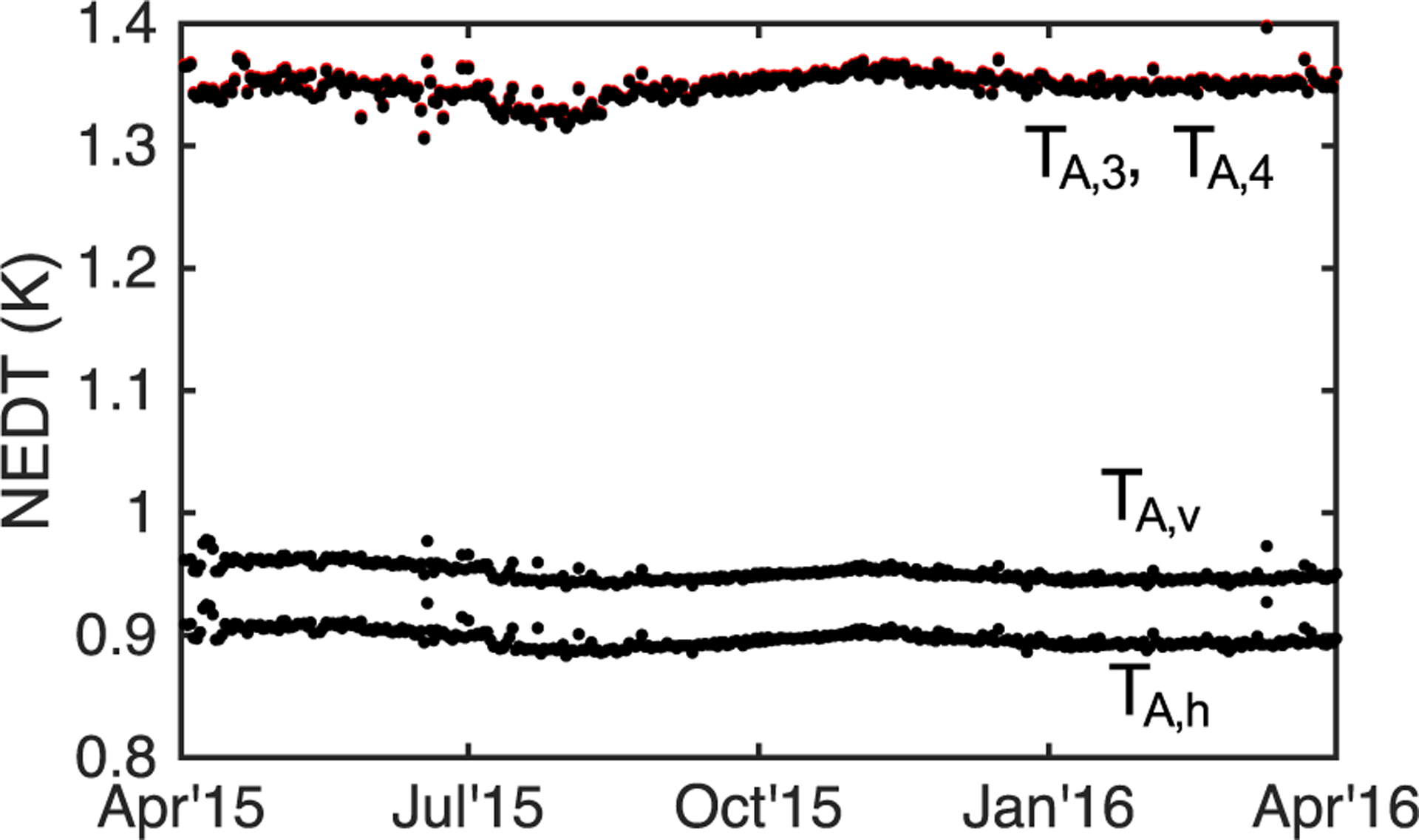
Radiometric resolution (NEDT) daily averaged (over land, ocean, and ice) during the first year of operations for all four Stokes brightness temperatures. The third and fourth Stokes parameters (top curves) have NEDT √2 larger than vertical and horizontal polarizations as expected.

Transient temperatures, particular those that cause changes in thermal gradients within the RFE, can cause drift in systematic calibration biases (in scale and/or offset). While the science-processing algorithm compensates for temperature effects, the model has residual uncertainty. The radiometer is thermally stabilized by passive thermal design and active thermal control to minimize the impacts of the changing thermal environment. Several platinum resistance thermometers (PRTs) are used to measure the temperatures and thermal stability of the radiometer components. The PRT measurements of the front end over the first year are shown in Fig. 14. Each PRT is read every 20 s and has 0.01 °C resolution and ±0.5 °C accuracy. During most of the past year and when under normal operating conditions, the temperatures are quite stable. The diplexers, couplers, and OMT are seen to vary <1 °C seasonally including during the South Pole solar eclipse season (May through July) in Fig. 14(a). Even if left uncompensated, the variation in calibration bias due to these front-end thermal variations is <0.1 K. The feed horn varies in temperature quite a bit more, about 14 °C peak to peak, but its ohmic loss is nearly negligible and varies 2 ppm/°C. The temperatures of the internal calibration sources have 0.4 °C peak to peak variation shown in Fig. 14(b). The internal noise source has a temperature coefficient of 3 ppt/°C (referred to the feedhorn), which results in a calibration dependence of 0.3 K that is compensated in the science-processing algorithm. The steps in temperature early in the operation year are due to various activities during the first two weeks of instrument commissioning. The occasional 1 °C impulses are due to instrument power cycling as a consequence of satellite operations. These power cycles do interrupt the calibration temporarily; however, the instrument recovers within a few orbits and returns to steady state thereafter.

Fig. 14.

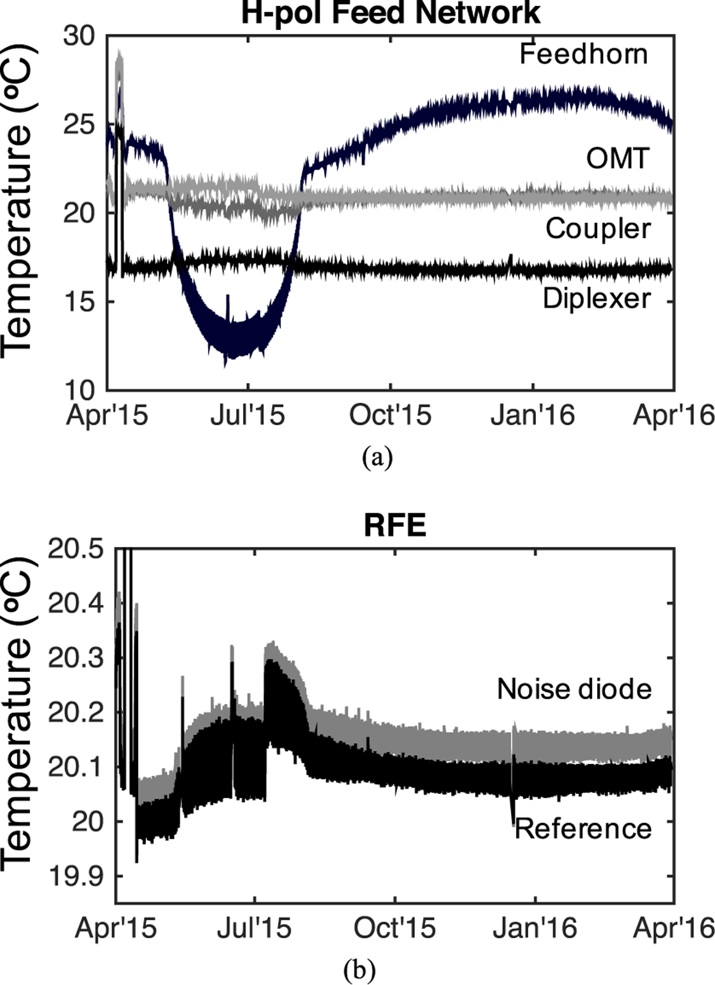
Temperatures of (a) feed network and (b) internal reference load and noise source for horizontal-polarization during the first year of operations.

The short-term orbital variations in temperature are shown in Fig. 15 for the worst-case peak of the eclipse season. During this orbit, the feedhorn varied 2 °C and the other feed network components 0.2 °C. The internal calibration sources varied 0.1 °C over the orbit. These variations have a negligible impact on the intraorbital stability of the receiver calibration.

Fig. 15.

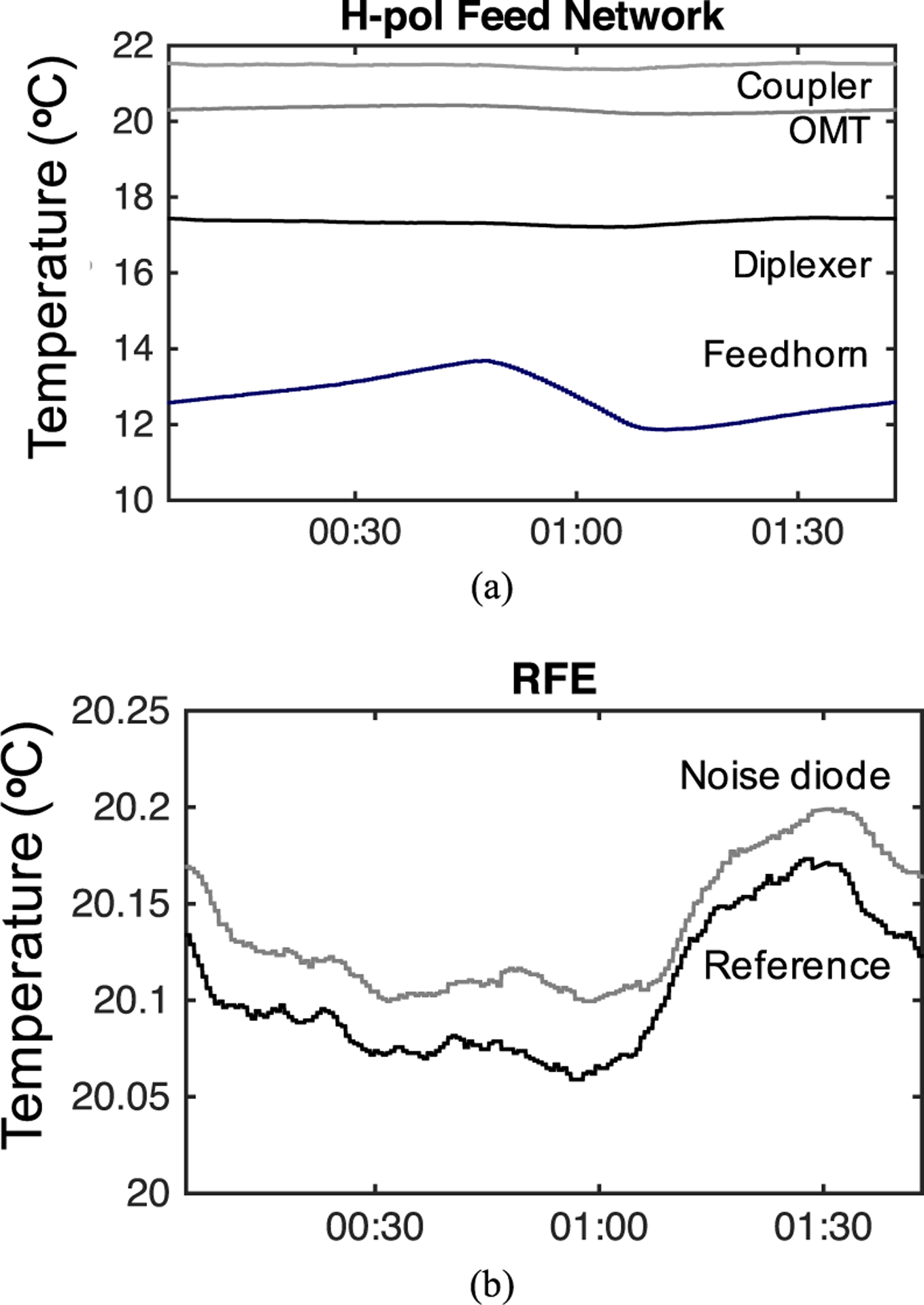
Temperatures of (a) feed network and (b) internal reference load and noise source for horizontal-polarization over on orbit on June 23, 2015 near the peak thermal effect of eclipse season.

Noise diode bias current and avalanche breakdown voltage are measured every eight days during normal operations and plotted in Fig. 16. The bias current is stable to 2 μA peak to peak and breakdown voltage 1.4 mV peak to peak. Based on laboratory measurements of diode components, the calibration dependence on these dc bias variations is 250 ppm.

Fig. 16.

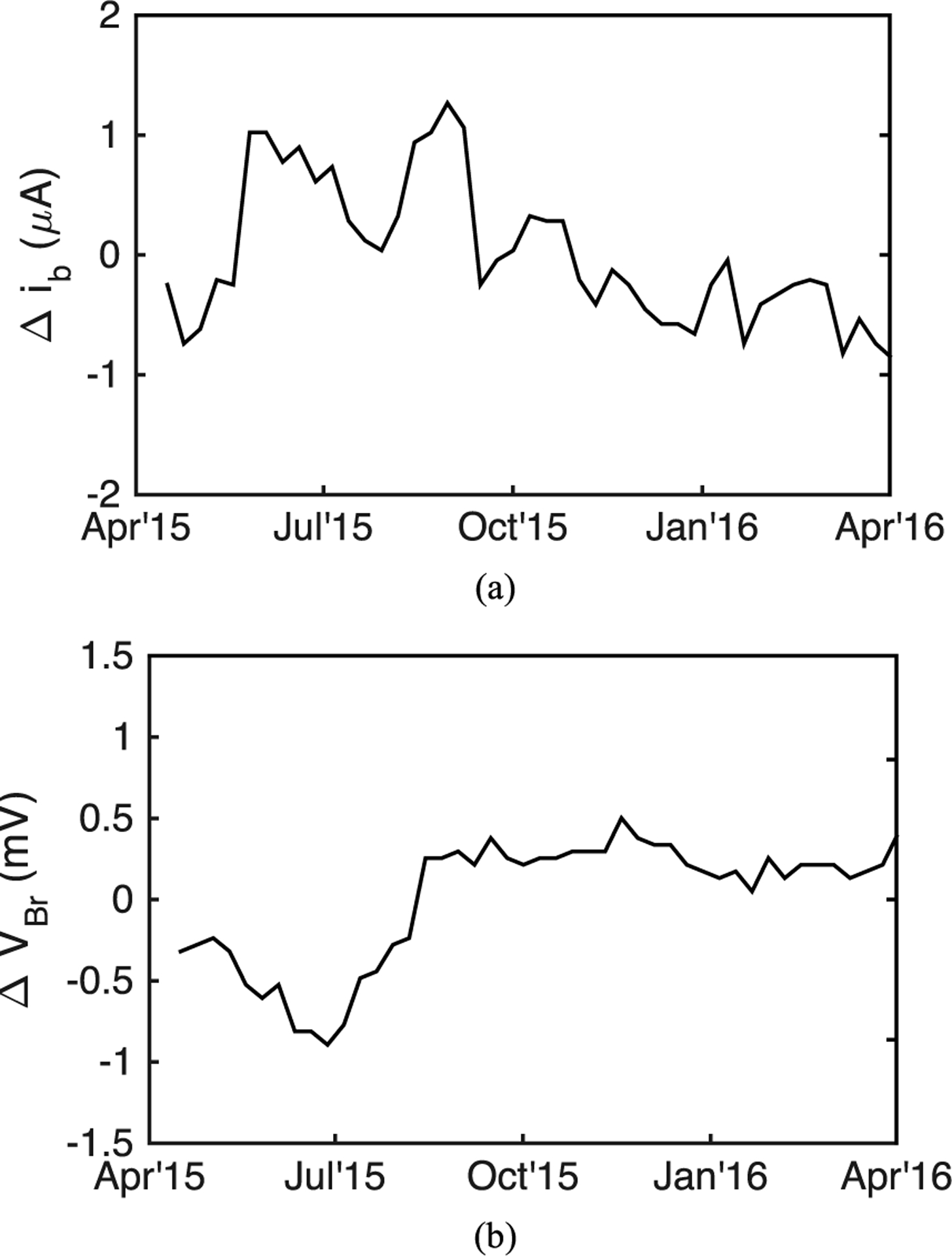
Noise source bias history measured on an eight-day period during the first year of operations. (a) Current bias variation is within ± 1.1 μA or ±180 ppm. (b) Avalanche voltage varies ±0.7 mV or ±80 ppm.

The combination of noise diode bias stability and thermal stability leads to excellent radiometer gain stability on orbital time scales. The radiometer switching provides noise diode and reference load counts every 8.4 ms. These are used to compute gain and offset coefficients with some corrections applied for temperature. The calibration coefficients are then averaged with a 5000-tap moving average window spanning 42 s of elapsed time. Thus, it is necessary for the hardware gain to be stable with periods <84 s, and so, the process Nyquist samples the hardware behavior. The gain spectrum and averaging filter response are shown in Fig. 17. The gain is stable (≪10⁻⁵) above 1 mHz (1000-s period), and so the 42-s filter is averaging over small fluctuations. The orbit period of 5900 s is marked for reference. The temperature correction algorithm compensates for orbital-scale dependence in gain. Below 1 mHz, the gain spectrum begins to rise with f ^−α-type behavior; however, this characteristic is fully captured by the calibration scheme.

Fig. 17.

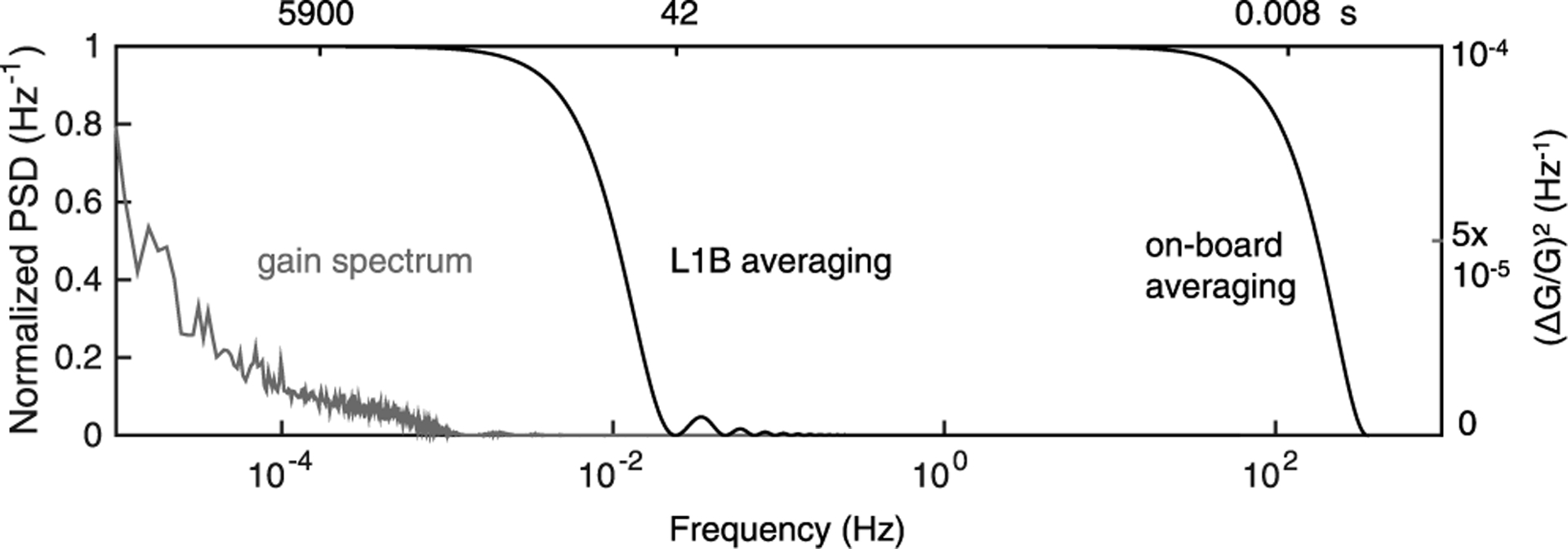
Radiometer gain stability and gain averaging filter responses. The rightmost trace is the response of the on-board sampling of noise-diode and reference counts every 8.4 ms. The science processing software averages 5000 gain estimates together, which span 42 s. The orbit cycle is marked at 5900 s. The spectrum of gain coefficient fluctuation, the left most trace, reveals an increasing spectrum below 1 MHz.

Noise diode calibration sources are known to drift on long timescales while on orbit [24] and this behavior was no exception on SMAP’s precursor Aquarius, which exhibited an exponential drift with 0.5% amplitude and 100-day time constant [25]. Noise source drift of 0.5% is equivalent to 1 K drift over the ocean. The calibration drift over land due to noise source drift is less, because the land antenna temperatures are closer to the internal reference load temperature. SMAP uses the same basic design as Aquarius for the noise sources, and so, long-term drift is expected and is being monitored. Because of the potentially long time constant of 100 days, it is too early to determine if SMAP is exhibiting exactly a similar behavior. Nonetheless, SMAP stability is monitored against a globally averaged ocean model (based on that described in [26]) with results reported in [27] and [29]. Calibration drift cast as a relative change in noise diode intensity is shown in Fig. 18. The lower curve shows the estimated drift including several steps downward and upward due to intentional and unintentional power cycles of the radar transmitter. The upper curve is an estimate of the drift due to changes in radiometer hardware over the year with the steps removed. The vertical dashed lines indicate the start and finish of solar eclipse season for the spacecraft during the southern hemisphere winter. The bump downward in calibration immediately after eclipse ends is likely due to some uncompensated front-end thermal effect. As discussed in [27] and [29], there remains uncertainty in radome and reflector emissivity that is confounded with noise source drift. The separation of the errors and correction thereof are topics of on-going calibration activities. Nonetheless, the stability of SMAP is consistent with Aquarius, although the physical mechanisms and temporal characteristics are not yet fully resolved.

Fig. 18.

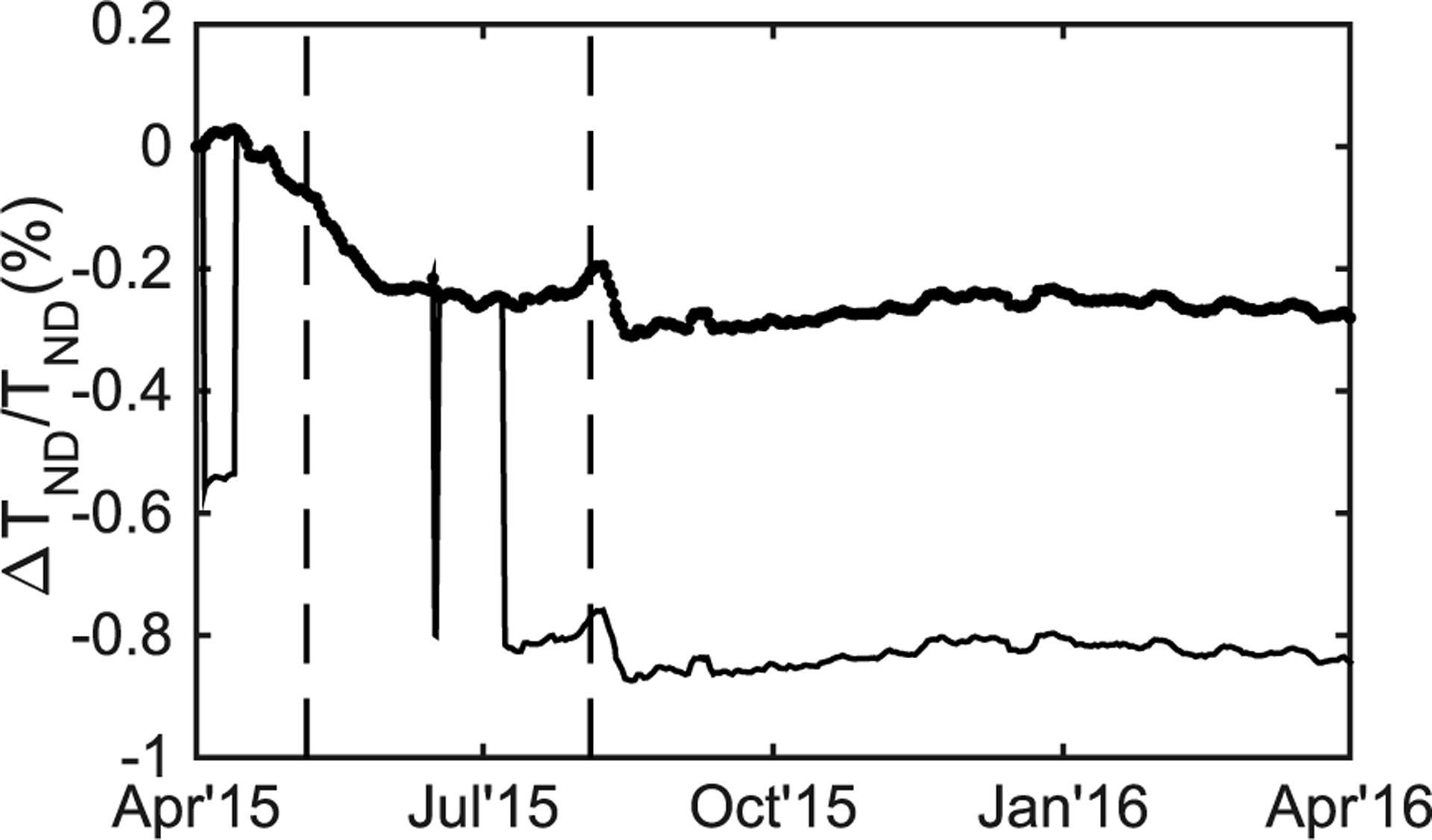
Radiometer calibration stability cast as gain drift during the first year of operation determined from comparison to globally averaged ocean model (lower curve). The two steps in April are due to intentional change in physical temperature during early commissioning activities. The step near June 14 was due to an intentional power cycle. The final large step in July was due to termination of radar transmission. The upper curve is the same noise source drift with the radar-induced steps removed. The vertical dashed lines indicated the start and finish of the solar eclipse season experienced by SMAP in the southern hemisphere winter.

VII. Stokes Imagery

SMAP provides global coverage with a three-day revisit on an eight-day repeat orbit cycle. Antenna temperature data averaged over one such cycle for all four modified Stokes parameters are shown in Fig. 19. These data are during the third week of April 2016 from [20]. The impact of moisture in the soil on antenna temperature in vertical and horizontal polarizations is quite evident across the northern hemisphere, including the Midwest and the State of Texas in the U.S. where extreme precipitation led to flooding resulting in low brightness temperatures 180–190 K shown in blue on the cool end of the color scale. Other physical features of note include the high emissivity of the Amazon rainforest and the dry Sahara shown in red at the warm end of the color scale. Note that the color scale was truncated at (168–282 K) to emphasize contrast in the antenna temperature of land. This truncation necessarily saturates at ocean antenna temperatures, where dominance of Fresnel reflectivity would otherwise be evident in contrast between vertical and horizontal polarizations. Strong contrast, however, is seen in the regions of sea ice with 190 and 230 K antenna temperatures at horizontal and vertical polarizations, respectively.

Fig. 19.

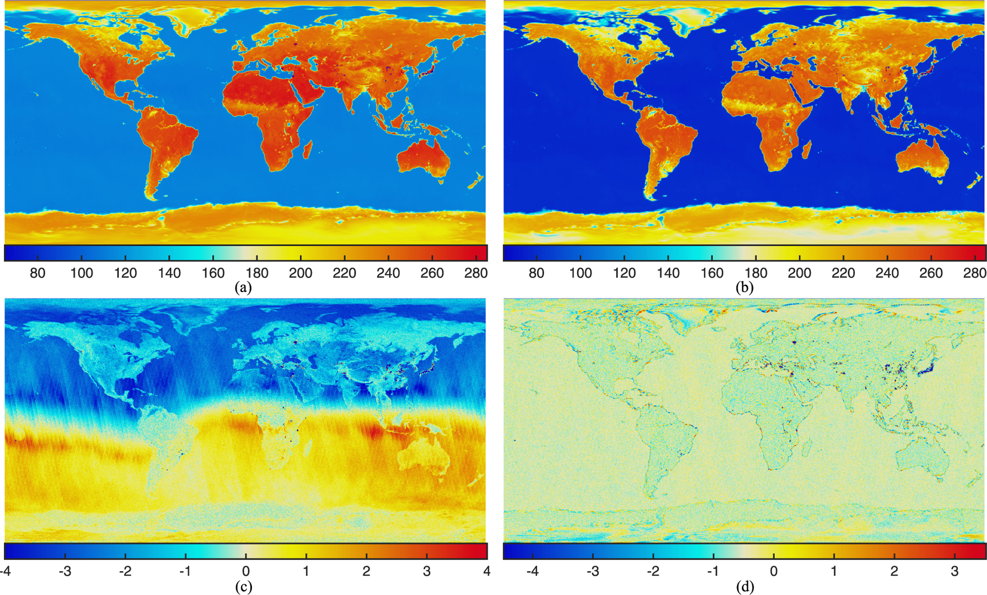
SMAP radiometer modified Stokes antenna temperatures gridded and averaged during September 1–7, 2015. The four panels show (a) vertically polarized, (b) horizontally polarized, (c) third, and (d) fourth Stokes parameters, respectively.

The third Stokes antenna temperature [Fig. 19(c)] shows a strong dipole feature caused by ionospheric Faraday rotation. The dipole in the third Stokes arises from the alignment of earth’s magnetic field with the direction of propagation of observed microwave emission. The amplitude of the third Stokes is the strongest over ocean because of the low emission and strong polarization caused by its Fresnel reflectivity and weaker over land (especially Amazon and Congo rainforests) due to higher emissivity and depolarization due to scattering. There are also artifacts in the image due to combining ascending and descending orbits. The fourth Stokes parameter, on the other hand, is nearly nonexistent in Fig. 19(d). The color scale is slightly offset to account for a global bias, likely due to antenna cross-polarization mixing. The continents are slightly more negative than ocean and their outlines are evident because of antenna cross-pol mixing, which couples some combination of the first and second into fourth Stokes. Finally, there are unique patterns of fourth Stokes antenna temperature over Greenland and Antarctica, perhaps vestiges of the polarimetric signature witnessed by WindSat [30].

VIII. Discussion

One year of nearly continuous operation of the SMAP L-band microwave radiometer was marked on March 31, 2016. Two key technologies—the 6-m scanning reflector and the radio frequency interference detection and filtering digital back end with polarimetric capabilities— combine to make the radiometer unique. Radiometer footprints sampled at 17-ms provide angular Nyquist sampling and exhibit NEDT <1 K. On-board calibration combined with good thermal stability yields excellent on-orbit gain stability. Global swath imagery of all four Stokes antenna temperatures shows good results. Vertical and horizontal polarized channels display expected behavior for land, ocean, and ice scenes. The third Stokes channel responds strongly to ionospheric Faraday rotation. The fourth Stokes channel indicates little circularly polarized emission, except over large ice sheets. The instrument continues to operate equally well as of this writing. Thus, the radiometer meets the key and driving mission requirements needed to measure soil moisture at 40-km spatial resolution and 0.04 volumetric uncertainty.

Biography

Jeffrey R. Piepmeier (S’93–M’99–SM’10) received the B.S.Eng. (summa cum laude) degree in electrical concentration from LeTourneau University, Longview, TX, USA, in 1993, and the M.S. and Ph.D. degrees in electrical engineering from the Georgia Institute of Technology, Atlanta, GA, USA, in 1994 and 1999, respectively.

He was with Vertex Communications Corporation, Kilgore, TX, and was a Schakleford Fellow with the Georgia Tech Research Institute, Atlanta. He was an Associate Head of Microwave Instruments and Technology, NASA Goddard Space Flight Center (GSFC), Greenbelt, MD, USA. He is currently the Chief Engineer of Passive Microwave Instruments with the Instrument Systems and Technology Division, NASA GSFC. He is also an Instrument Scientist or the Soil Moisture Active Passive Microwave Radiometer and the GPM Microwave Imager. He is a member of the Aquarius Science Team. His current research interests include microwave radiometry and technology development to enable the next generation of microwave sensors.

Dr. Piepmeier is a member of the International Union of Radio Science and the American Geophysical Union. He is a former Chairperson of the National Academies’ Committee on Radio Frequencies. He was a recipient of the NASA Outstanding Leadership Medal for contributions to NASA’s microwave radiometer missions, the NASA Exceptional Engineering Achievement Medal for advances in RFI mitigation technology for microwave radiometers, the NASA Exceptional Achievement Medal for significant contributions to the Aquarius/SAC-D mission, and six NASA Group Achievement Awards.

Paolo Focardi (M’03–SM’15) received the M.Sc. degree in electronic engineering and the Ph.D. degree in computer science and telecommunication engineering from the University of Florence, Florence, Italy, in 1998 and 2002, respectively.

From 1999 to 2000, he was involved in the Shuttle Radar Topography Mission in collaboration with the Italian Space Agency, Rome, Italy. In 2001, he visited the NASA’s Jet Propulsion Laboratory (JPL), Pasadena, CA, USA, where he was involved in the development of an accurate electromagnetic model of THz detectors. In 2002, he joined the staff of JPL and became a Staff Engineer in 2014. From 2004 to 2009, he was involved in a project to remotely detect human vital signs that in 2009 led to the creation of a start-up company, Advanced TeleSensors Inc., Pasadena, CA. In 2008, he supported the development of the A1 and A2 antennas for JUNO and then he joined the RF team, developing the instrument reflector antenna for Soil Moisture Active Passive (SMAP). In 2009, he joined the Spacecraft Antennas Group, JPL, and in 2010, he started the design of the feed horn assembly for SMAP and was able to model the entire spacecraft in order to get very accurate predictions of the radiation pattern. He is currently responsible for the design and delivery of the NISAR feed assembly. He is involved in analytical and numerical methods in electromagnetism for the analysis and design of RF circuits and antennas. He has authored or co-authored Chapter 8 of the Space Antenna Handbook (Wiley, 2012), another chapter of Handbook of Modern Reflector Antennas and Feed Systems for Space and Ground Applications (Artech House, 2013), and over 40 publications in the most renowned national and international journals.

Dr. Focardi serves as a Reviewer of many renowned national and international journals.

Kevin A. Horgan (M’16) received the B.S.E.E. and M.S.E.E. degrees from the University of Massachusetts, Amherst, MA, USA, in 1999 and 2003, respectively.

Since 2003, he has been with the Microwave Instrument Technology Branch, NASA Goddard Space Flight Center, Greenbelt, MD, USA. From 2004 to 2008, he designed microstrip circuits and delivered flight-qualified RF assemblies for the Aquarius mission. From 2008 to 2013, he was the Product Development Lead (PDL) of the Soil Moisture Active Passive (SMAP) Radiometer RF Electronics. From 2013 to 2015, he supported SMAP through Assembly Test Launch Operations and on-orbit commissioning. From 2014 to 2015, he served as the Integration and Test Lead for the IceCube sub-millimeter wave instrument. Since 2016, he has been the PDL for the RF Electronics for the CubeSat Radiometer Radio Frequency Interference Technology Validation (CubeRRT) mission.

Joseph Knuble is currently with the NASA Goddard Space Flight Center, Greenbelt, MD, USA, and led the development of the soil moisture active passive radiometer RF front-end.

Negar Ehsan (S’05–M’10) received the B.S. and M.S. degrees in electrical engineering with a minor in applied mathematics, in 2006, and the Ph.D. degree in electrical engineering from the University of Colorado at Boulder, Boulder, CO, USA, in 2010.

Since 2010, she has been with the NASA Goddard Space Flight Center, Greenbelt, MD, USA, where she currently serves as the IceCube Mission Instrument Lead and a System Engineer. She has been involved in both flight and research projects with applications in earth science and astrophysics. She has served as a Principal Investigator on several internal research and development projects, which resulted in several patents pending. Her current research interests include millimeter- and submillimeter-wave radiometry, passive and active broadband microwave circuits, millimeter-wave antennas and arrays, and terahertz components for space flight missions.

Dr. Ehsan was a recipient of the Win New Work Award for significant contributions in efforts to bring strategic in-house work to the Applied Engineering Technology Directorate.

Jared Lucey was a Microwave Engineer with the Soil Moisture Active Passive Radiometer Team responsible for the antenna feed network. He is currently with the NASA Goddard Space Flight Center, Greenbelt, MD, USA.

Clifford Brambora is currently with the NASA Goddard Space Flight Center, Greenbelt, MD, USA, and led the development of the soil moisture active passive radiometer digital electronics.

Paula R. Brown was the Lead Antenna RF Engineer of the Soil Moisture Active Passive Instrument. She is currently with the NASA Jet Propulsion Laboratory, Pasadena, CA, USA.

Pamela J. Hoffman was the Mechanical and Thermal Element Manager of the Soil Moisture Active Passive Instrument. She is currently with the NASA Jet Propulsion Laboratory, Pasadena, CA, USA.

Richard T. French was the Spin Subsystem System Engineer of the Soil Moisture Active Passive Instrument. He is currently with the NASA Jet Propulsion Laboratory, Pasadena, CA, USA.

Rebecca L. Mikhaylov was the Thermal Analysis Engineer of the Soil Moisture Active Passive Instrument. She is currently with the NASA Jet Propulsion Laboratory, Pasadena, CA, USA.

Eug-Yun Kwack was the Lead Thermal Engineer of the Soil Moisture Active Passive Instrument. He is currently with the NASA Jet Propulsion Laboratory, Pasadena, CA, USA.

Eric M. Slimko was the Lead Mechanical System Engineer of the Soil Moisture Active Passive Instrument. He is currently with the NASA Jet Propulsion Laboratory, Pasadena, CA, USA.

Douglas E. Dawson was an Instrument System Engineer of the Soil Moisture Active Passive Radiometer. He is currently with the NASA Jet Propulsion Laboratory, Pasadena, CA, USA.

Derek Hudson was the Calibration Engineer of the Soil Moisture Active Passive Radiometer. He is currently with the NASA Goddard Space Flight Center, Greenbelt, MD, USA.

Jinzheng Peng received the B.S. degree in electrical engineering from Wuhan University, Wuhan, China, the M.S. degree in electrical and computer engineering from the University of Massachusetts, Amherst, MA, USA, and the Ph.D. degree in electrical engineering from the University of Michigan, Ann Arbor, MI, USA.

From 1991 to 2000, he was with the Beijing Institute of Remote Sensing Equipment, Beijing, China. He is currently with Goddard Earth Sciences Technology and Research, Universities Space Research Association, Columbia, MD, USA, and with the NASA’s Goddard Space Flight Center, Greenbelt, MD, USA. He is currently involved in algorithm development and calibration/validation for the Soil Moisture Active/Passive Radiometer. His current research interests include system-level concept design, analysis, calibration/validation, and algorithm development for microwave remote-sensing instruments.

Priscilla N. Mohammed (S’02–M’06) received the B.S. degree from the Florida Institute of Technology, Melbourne, FL, USA, in 1999, and the M.S. and Ph.D. degrees from the Georgia Institute of Technology, Atlanta, GA, USA, in 2001 and 2005, respectively, all in electrical engineering. As a Ph.D. student, she performed microwave measurements of gaseous phosphine and ammonia under simulated conditions for the outer planets and used these measurements to develop a radio occultation simulator to predict absorption and excess Doppler due to Saturn’s atmosphere. Much of this work was in support of the Cassini mission to Saturn. Based on these laboratory results, the Cassini Project Science Group made the decision to extend the Ka-band (32 GHz) operation throughout the mission tour.

She is currently with Goddard Earth Sciences Technology and Research, Universities Space Research Association, Columbia, MD, USA, as a member of Morgan State University research faculty and with the Microwave Instrument Technology Branch, NASA’s Goddard Space Flight Center, Greenbelt, MD. She is also a member of the Algorithm Development Team for the Soil Moisture Active Passive Radiometer. Her current research interests include radio frequency interference mitigation in microwave radiometers.

Giovanni De Amici is currently with the NASA Goddard Space Flight Center, Greenbelt, MD, USA, and also a member of the Soil Moisture Active Passive Radiometer Calibration Team.

Adam P. Freedman received the B.S. degree in physics from Yale University, New Haven, CT, USA, in 1980, and the Ph.D. degree in marine geophysics from the Massachusetts Institute of Technology, Cambridge, CA, USA, in 1987.

He joined the technical staff at the NASA Jet Propulsion Laboratory, Pasadena, CA, USA, where he was involved in earth rotation studies until 1996. He was involved in the Radar Sciences Section, first on the GeoSAR airborne X- and P-band radar platform, then as an Instrument System Engineer of the Aquarius Project, and later as the Instrument Operations Team Lead of the Soil Moisture Active Passive Mission. He is currently a System Engineer of the REASON Europa Sounding Radar.

Dr. Freedman is a member of Sigma Xi and the American Geophysical Union.

James Medeiros was an Instrument System Engineer of the Soil Moisture Active Passive Radiometer. He is currently with the NASA Goddard Space Flight Center, Greenbelt, MD, USA.

Fred Sacks was with Base2 Engineering at the NASA Goddard Space Flight Center, Greenbelt, MD, USA, and was an RF System Engineer of the Soil Moisture Active Passive Radiometer.

Robert Estep was an Instrument Manager of the Soil Moisture Active Passive Radiometer. He is currently with the NASA Goddard Space Flight Center, Greenbelt, MD, USA.

Michael W. Spencer was an Instrument System Engineer of the Soil Moisture Active Passive Instrument. He is currently with the NASA Jet Propulsion Laboratory, Pasadena, CA, USA.

Curtis W. Chen received the B.S. and A.B. degrees in electrical engineering and political science, and the M.S. and Ph.D. degrees in electrical engineering from Stanford University, Stanford, CA, USA, in 1996, 1999, and 2001, respectively, where he developed new algorithms for 2-D phase unwrapping of interferometric SAR data.

Since 2001, he has been with NASA Jet Propulsion Laboratory, Pasadena, CA, USA, where he was involved in radars for Mars landers and Earth-science instruments. He was the Lead System Engineer of the Soil Moisture Active Passive combined active/passive instrument system from subsystem integration through launch.

Kevin B. Wheeler was an Instrument System Engineer of the Soil Moisture Active Passive instrument. He is currently with the NASA Jet Propulsion Laboratory, Pasadena, CA, USA.

Wendy N. Edelstein was an Instrument Manager of the Soil Moisture Active Passive instrument. She is currently with the NASA Jet Propulsion Laboratory, Pasadena, CA, USA.

Peggy E. O’Neill (F’16) received the B.S. (summa cum laude) degree (Hons.) in geography from Northern Illinois University, DeKalb, IL, USA, in 1976, and the M.A. degree in geography from the University of California at Santa Barbara, Santa Barbara, CA, USA, in 1979.

She has done postgraduate work in civil and environmental engineering with Cornell University, Ithaca, NY, USA. Since 1980, she has been a Physical Scientist with the Hydrological Sciences Laboratory, NASA’s Goddard Space Flight Center, Greenbelt, MD, USA, where she conducts research in soil moisture retrieval and land surface hydrology, primarily through microwave remote sensing techniques. She is currently the Soil Moisture Active Passive Deputy Project Scientist at NASA GSFC, Greenbelt, MD USA.

Eni G. Njoku (M’75–SM’83–F’95) received the B.A. degree in natural and electrical sciences from Cambridge University, U.K., in 1972, and the M.S. and Ph.D. degrees in electrical engineering from the Massachusetts Institute of Technology, Cambridge, MA, USA, in 1974 and 1976, respectively.

He was a Senior Research Scientist with the Surface Hydrology Group, NASA Jet Propulsion Laboratory, California Institute of Technology, Pasadena, CA, USA, until his retirement in 2016. His current research interests include passive and active microwave sensing of soil moisture for hydrology and climate applications. He was the Project Scientist of the Soil Moisture Active Passive mission from 2008 to 2013 and a member of the U.S. Advanced Microwave Scanning Radiometer Science Team.

Dr. Njoku was a recipient of the NASA Exceptional Public Service Medal in 2016.

References

- [1].Entekhabi D et al. , “The Soil Moisture Active Passive (SMAP) mission,” Proc. IEEE, vol. 98, no. 5, pp. 704–716, May 2010. [Google Scholar]
- [2].Kerr YH et al. , “The SMOS mission: New tool for monitoring key elements of the global water cycle,” Proc. IEEE, vol. 98, no. 5, pp. 666–687, May 2010. [Google Scholar]
- [3].Lagerloef G et al. , “The Aquarius/SAC-D mission: Designed to meet the salinity remote-sensing challenge,” Oceanography, vol. 21, no. 1, pp. 68–81, March 2008. [Google Scholar]
- [4].National Research Council, Earth Science and Applications from Space: National Imperatives for the Next Decade and Beyond. Washington, DC, USA: Nat. Acad. Press, 2007. [Online]. Available: 10.17226/11820. [DOI] [Google Scholar]
- [5].Entekhabi D et al. , “The Hydrosphere State (hydros) satellite mission: An earth system pathfinder for global mapping of soil moisture and land freeze/thaw,” IEEE Trans. Geosci. Remote Sens, vol. 42, no. 10, pp. 2184–2195, October 2004. [Google Scholar]
- [6].NASA/JPL, NASA Soil Moisture Radar Ends Operations, Mission Science Continues, accessed on Mar. 18, 2016 [Online]. Available: http://www.jpl.nasa.gov/news/news.php?feature=4710
- [7].Mohammed PN, Aksoy M, Piepmeier JR, Johnson JT, and Bringer A, “SMAP L-band microwave radiometer: RFI mitigation prelaunch analysis and first year on-orbit observations,” IEEE Trans. Geosci. Remote Sens, vol. 54, no. 10, pp. 6035–6047, October 2016. [Google Scholar]
- [8].Gaiser PW et al. , “The WindSat spaceborne polarimetric microwave radiometer: Sensor description and early orbit performance,” IEEE Trans. Geosci. Remote Sens, vol. 42, no. 11, pp. 2347–2361, November 2004. [Google Scholar]
- [9].Kawanishi T et al. , “The Advanced Microwave Scanning Radiometer for the Earth Observing System (AMSR-E), NASDA’s contribution to the EOS for global energy and water cycle studies,” IEEE Trans. Geosci. Remote Sens, vol. 41, no. 2, pp. 184–194, February 2003. [Google Scholar]
- [10].Vine DML, Lagerloef GSE, Colomb FR, Yueh SH, and Pellerano FA, “Aquarius: An instrument to monitor sea surface salinity from space,” IEEE Trans. Geosci. Remote Sens, vol. 45, no. 7, pp. 2040–2050, July 2007. [Google Scholar]
- [11].Brown S, Ruf C, Keihm S, and Kitiyakara A, “Jason microwave radiometer performance and on-orbit calibration,” Marine Geodesy, vol. 27, nos. 1–2, pp. 199–220, 2004. [Google Scholar]
- [12].Misra S and Ruf CS, “Detection of radio-frequency interference for the Aquarius radiometer,” IEEE Trans. Geosci. Remote Sens, vol. 46, no. 10, pp. 3123–3128, October 2008. [Google Scholar]
- [13].Piepmeier JR et al. , “Radio-frequency interference mitigation for the Soil Moisture Active Passive Microwave radiometer,” IEEE Trans. Geosci. Remote Sens, vol. 52, no. 1, pp. 761–775, January 2014. [Google Scholar]
- [14].Piepmeier JR and Gasiewski AJ, “Digital correlation microwave polarimetry: Analysis and demonstration,” IEEE Trans. Geosci. Remote Sens, vol. 39, no. 11, pp. 2392–2410, November 2001. [Google Scholar]
- [15].O’Neill PE, Njoku EG, Jackson TJ, Chan S, and Bindlish R, “SMAP algorithm theoretical basis document: Level 2 & 3 soil moisture (passive) data products,” Jet Propuls. Lab., California Inst. Technol, Pasadena, CA, USA, Tech. Rep. JPL D-66480, 2015 [Online]. Available: http://nsidc.org/data/docs/daac/smap/sp_l2_smp/index.html [Google Scholar]
- [16].Yueh SH, “Estimates of Faraday rotation with passive microwave polarimetry for microwave remote sensing of earth surfaces,” IEEE Trans. Geosci. Remote Sens, vol. 38, no. 5, pp. 2434–2438, September 2000. [Google Scholar]
- [17].Piepmeier JR et al. , “SMAP algorithm theoretical basis document: L1B radiometer product. SMAP project, NASA GSFC SMAPALGMS-RPT-006 Rev. B,” NASA Goddard Space Flight Center, Greenbelt, MD, USA, Tech. Rep, February 2016. [Online.] Available: http://nsidc.org/data/docs/daac/smap/sp_l1b_tb/index.html [Google Scholar]
- [18].Ruf CS, Keihm SJ, and Janssen MA, “TOPEX/Poseidon Microwave Radiometer (TMR). I. Instrument description and antenna temperature calibration,” IEEE Trans. Geosci. Remote Sens, vol. 33, no. 1, pp. 125–137, January 1995. [Google Scholar]
- [19].Peng J and Ruf CS, “Calibration method for fully polarimetric microwave radiometers using the correlated noise calibration standard,” IEEE Trans. Geosci. Remote Sens, vol. 46, no. 10, pp. 3087–3097, October 2008. [Google Scholar]
- [20].Johnson C, “Temperature stability and control requirements for thermal vacuum/thermal balance testing of the Aquarius radiometer,” in Proc. 25th Space Simulation Conf, Annapolis, MD, USA, October 2008, pp. 20–23. [Google Scholar]
- [21].Piepmeier JR, Mohammed P, Peng J, Kim EJ, De Amici G, and Ruf C, SMAP L1B Radiometer Half-Orbit Time-Ordered Brightness Temperatures, Version 3. Boulder, CO, USA: NASA Nat. Snow and Ice Data Center Distributed Active Archive Center, Mar./Apr. 2015. [Online]. Available: 10.5067/YV5VOWY5V446 [DOI] [Google Scholar]
- [22].Mastropietro A et al. , “Preliminary evaluation of passive thermal control for the soil moisture active and passive (SMAP) radiometer,” in Proc. 41st Int. Conf. Environ. Syst., Int. Conf. Environ. Syst. (ICES), 2011. [Online]. Available: 10.2514/6.2011-5070 [DOI] [Google Scholar]
- [23].Mikhaylov R et al. , “Implementation of active thermal control (ATC) for the soil moisture active and passive (SMAP) radiometer,” in Proc. 44th Int. Conf. Environ. Syst., Int. Conf. Environ. Syst. (ICES), 2014. [Online]. Available: http://hdl.handle.net/2346/59511 [Google Scholar]
- [24].Brown ST, Desai S, Lu W, and Tanner A, “On the long-term stability of microwave radiometers using noise diodes for calibration,” IEEE Trans. Geosci. Remote Sens, vol. 45, no. 7, pp. 1908–1920, May 2007. [Google Scholar]
- [25].Piepmeier JR, Hong L, and Pellerano FA, “Aquarius L-band microwave radiometer: 3 years of radiometric performance and systematic effects,” IEEE J. Sel. Topics Appl. Earth Obs. Remote Sens, vol. 8, no. 12, pp. 5416–5423, December 2015. [Google Scholar]
- [26].Wentz FJ and LeVine DM, “Algorithm theoretical basis document: Aquarius salinity retrieval algorithm,” Remote Sens. Syst, Santa Rosa, CA, USA, Tech. Rep. 082912, 2012. [Google Scholar]
- [27].Piepmeier JR et al. , “SMAP radiometer brightness temperature calibration for the L1B_TB and L1C_TB beta-level data products,” NASA’s SMAP Project, Jet Propuls. Lab, Pasadena, CA, USA, Tech. Rep. D-93978, July 2015. [Online]. Available: https://nsidc.org/data/smap/data_versions [Google Scholar]
- [28].Piepmeier JR et al. , “SMAP radiometer brightness temperature calibration for the L1B_TB and L1C_TB version 2 data products,” NASA’s SMAP Project, Jet Propuls. Lab, Pasadena, CA, USA, November 2015. [Online]. Available: https://nsidc.org/data/smap/data_versions [Google Scholar]
- [29].Piepmeier JR et al. , “SMAP radiometer brightness temperature calibration for the L1B_TB and L1C_TB version 3 data products,” NASA’s SMAP project, Jet Propuls. Lab, Pasadena, CA, USA, April 2016. [Online]. Available: https://nsidc.org/data/smap/data_versions [Google Scholar]
- [30].Li L, Gaiser P, Albert MR, Long DG, and Twarog EM, “WindSat passive microwave polarimetric signatures of the Greenland ice sheet,” IEEE Trans. Geosci. Remote Sens, vol. 46, no. 9, pp. 2622–2631, September 2008. [Google Scholar]