Earth Observation-Based Ecosystem Services Indicators for National and Subnational Reporting of the Sustainable Development Goals

Abstract

Decision-making that impacts sustainability occurs at national and subnational levels, highlighting the need for multi-scale Earth observations (EO) and geospatial data for assessing the United Nations’ Sustainable Development Goals (SDGs). EnviroAtlas, developed by the United States Environmental Protection Agency and partners, provides a collection of web-based, interactive maps of environmental and socio-economic data relevant to the SDGs. EnviroAtlas maps ecosystem services indicators at national, regional, and local extents that can contribute to targets set forth in numerous goals, such as SDG 6 for clean water, SDG 11 for sustainable cities and communities, and SDG 15 for life on land. Examples of EnviroAtlas indicators that provide a way to view spatial inequalities, help fill gaps in environmental indicators, and integrate socio-economic and environmental data for the SDGs are explored herein. Remotely sensed EO data are essential for producing these indicators and informing planning and decision-making for the SDGs at subnational scales. The National Land Cover Dataset is the basis for many EnviroAtlas maps at the national extent, while National Agriculture Imagery Program and Light Detection and Ranging (LiDAR) data are used to classify Meter-scale Urban Land Cover in select US metro areas. These 30 meter and 1 meter land cover products are combined with demographic and other geospatial data (remotely sensed and otherwise) to produce integrated indicators that can aid in target setting of the SDGs. Though EnviroAtlas was created for the conterminous US, the methods for indicator creation are transferable, and the open-source code for the EnviroAtlas resource may serve as an example for other nations. Achieving the SDGs means assessing targets and decision-making outcomes at local, regional, and national levels using consistent and accurate data. Geospatial resources like EnviroAtlas that provide open access to indicators based on EO data and allow for assessment at multiple extents and resolutions are critical to broadly addressing national to subnational SDG goals and targets.

1. Introduction

As part of the United Nations’ 2030 Agenda for Sustainable Development adopted in 2015, nations agreed to voluntary and country-led efforts to monitor and work toward achieving the Sustainable Development Goals (SDGs). The SDG framework has 17 goals and 169 targets that focus on people, planet, prosperity, peace, and partnership whose interlinkages or integrated nature are key to realizing the Agenda. Now in its fifth year of global reporting, the framework measures annual progress with over 230 indicators that continue to be reviewed, added, and reported depending on data availability by country. Clause 74 of the Agenda lays out guiding principles for the follow-up and review process of adding new indicators or reporting with new data:

f. They [SDG indicators] will build on existing platforms and processes, where these exist, avoid duplication and respond to national circumstances, capacities, needs and priorities. They will evolve over time, taking into account emerging issues and the development of new methodologies, and will minimize the reporting burden on national administrations.

g. They will be rigorous and based on evidence, informed by country-led evaluations and data which is high-quality, accessible, timely, reliable and disaggregated by income, sex, age, race, ethnicity, migration status, disability and geographic location and other characteristics relevant in national contexts.

For indicator development, remotely sensed Earth observations (EO) play an increasingly important role in consistently measuring spatial and temporal attributes related to the SDGs (in this paper, EO refers to “remotely sensed” Earth observations). Many programs providing EO-based data products already exist, with some providing raw data (e.g., NASA’s Landsat Thematic Mapper, Copernicus Sentinel) and others providing derived data products (e.g., land cover, elevation). Data can be aggregated by geographic units from subnational to national levels. As discussed below, EO-based data can help fill three main gaps that currently exist in SDG indicators (Griggs et al., 2014; Scot and Rajabifard, 2017): 1) multi-resolution spatial indicators, 2) environmental indicators, and 3) indicators integrating environmental and societal or economic data. In this paper, we will use EnviroAtlas as an example of an online geospatial data resource and present several EO-derived metrics demonstrating how they could be used to complement existing SDG indicators and inform SDG goals and targets.

1.1. Sustainable Development Goals

1.1a. Multi-Resolution Spatial Indicators

Across countries, target setting in the SDGs is generally associated with temporal limits, starting with verbiage such as “By 2020…” or “By 2030…”. The current global system is based on reporting nationally aggregated indicators (i.e., one value per indicator per nation) (Sachs et al., 2018). The nationally aggregated indicators are critical for comparing values between nations and evaluating conditions across the globe. However, EO data provide opportunities for the development of scalable indicators allowing not only national reporting but also subnational reporting. Subnational reporting provides the tools for local or regional stakeholders and decision-makers to affect change on the ground.

Efforts to localize the SDGs and provide subnational reporting frameworks require attention to both the temporal and spatial resolution of SDG indicators. EO-based indicators expand possibilities for evaluating high and low performing geographic areas, providing a relatively low-cost mechanism for monitoring change, and meeting goals and targets by reducing spatial inequalities at multiple scales (Lucci, 2015). Advantages of using EO data for multi-resolution SDG indicators include capabilities for long-term monitoring and comparisons across communities, regions, and nations (Cord et al., 2017).

1.1b. Environmental Indicators

Based on the definition of sustainable development by Griggs et al. (2014), environmental indicators are foundational for monitoring current and future human health and well-being. Surprisingly, the current SDG framework has few environmental (or integrated indicators incorporating environmental) data compared to other frameworks originally proposed to the UN (Griggs et al., 2014). Of the 232 internationally agreed-upon indicators, only 46 are environmental, socio-environmental, or socio-economic-environmental according to our interpretation.

Though it is difficult to acquire reliable and accessible data for certain environmental indicators to feed into international indices and sustainability assessments (Dizdaroglu, 2017), EO data offer increasing opportunities for including environmental indicators at different scales around the globe. EO can provide stand-alone measurements of SDG indicators or can be combined with other sources of data (e.g., field monitoring, demographic) for integrated measurements. Furthermore, the current wording of the SDG targets allows for the consideration and addition of environmental as well as integrated indicators, such as ecosystem services indicators from EnviroAtlas described below.

1.1c. Integrated Indicators

Integrated indicators, as the term implies, integrate data from biophysical, social and economic spheres. The recent focus on ecosystem services, often defined as “the benefits people obtain from ecosystems” (MEA, 2005) has prompted the development of many integrated indicators. Ecosystem services science has required the integration of data from multiple disciplines to elucidate the direct and indirect benefits humans receive from nature (Boyd and Banzhaf, 2007). Ecosystem services indicators are measures that convey information about ecosystem service(s) production, supply, delivery to people, contribution to human well-being, or value (Brown et al., 2014), or some combination of these. Guidance for developing ecosystem services indicators can be found in Brown et al. (2014) and Müller and Burkhard (2012).

Ecosystem services frameworks fit with sustainability frameworks (Wu, 2013) and encompass most goals in the SDG framework as shown in Figure 1. Though there has been growing knowledge of ecosystem services concepts (Albert et al., 2014) and the use of EO for quantifying ecosystem services indicators (de Araujo Barbosa et al., 2015), their deliberate incorporation into sustainable development is still in early stages. A survey of field experts to assess the role of ecosystem services in the SDGs was conducted by Wood et al. (2018), and the results from survey respondents showed broad support for the contribution of ecosystem services indicators to 12 SDGs and 41 targets. The recognition of the critical role of ecosystem services to the SDGs by the United Nations Environmental Program is evident in the theme selected for the Fifth Session of the UN Environment Assembly (UNEA-5) currently scheduled to take place in 2021 in Nairobi, Kenya, Strengthening Actions for Nature to Achieve the Sustainable Development Goals (http://web.unep.org/environmentassembly/) .

Figure 1.

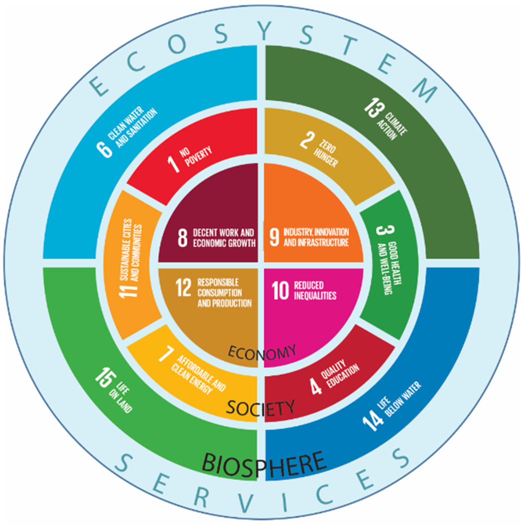
An Ecosystem Services framework connects all spheres of sustainability: Biosphere, Society and Economy. Targets in 14 of the 17 Sustainable Development Goals relate to an ecosystem services framework and can be addressed by or connected with ecosystem services indicators.

So far, Geijzendorffer et al. (2017) find that the ecosystem services indicators considered in the SDGs are biased toward ecosystem services supply, failing to incorporate socio-economic aspects of demand, use, and governance. EO data for land use and land cover change are commonly used for generating environmental indicators of ecosystem services supply. When combined with socio-economic data, ecosystem services demand can be determined, and integrated indicators created. These indicators can be translated to monetary and non-monetary benefits through surveys, interviews, and models. Integrating environmental and socio-economic data produces the strongest indicators for evaluating both ecosystem services and SDGs (Cord et al., 2017; Geijzendorffer et al., 2017; Griggs et al., 2014).

However, spatial and temporal resolutions of socio-economic data can be barriers to producing integrated indicators for ecosystem services and SDGs. National socio-economic data often have coarser spatial and temporal resolution than EO data. While some EO data are now produced in near-real-time, socio-economic data at subnational scales continue to be collected and compiled on multi-year or decadal timeframes (e.g., annual American Community Survey data released in 3- to 5-year summaries, decadal US census), thus impeding integration despite the availability of high-quality EO data.

1.2. EnviroAtlas

As part of the United States (US) Environmental Protection Agency’s (EPA’s) Sustainable and Healthy Communities research program, EnviroAtlas was created by the EPA and partners to provide nationally consistent geospatial indicators of ecosystem goods and services for the US. Data related to ecosystem services supply, demand, and drivers of change are available for the conterminous US (i.e. lower 48 states) via interactive mapping technology that allows for viewing, manipulating, and downloading data at multiple spatial resolutions by ecosystem services and geographic area (Pickard et al., 2015). Compared to other ecosystem services indicator tools, like parameterized models and libraries, EnviroAtlas is a web resource supported by a government agency for exploring ecosystem services maps and viewing ecosystem services case studies that address multiple policy sectors (Grêt-Regamey et al., 2017). Of the 68 ecosystem services tools reviewed by Grêt-Regamey et al. (2017), EnviroAtlas is one of only five tools that addresses air quality as an ecosystem service. EnviroAtlas allows users with no more than an internet browser to access a wealth of spatially explicit data that are readily reconfigurable and usable for measuring progress toward SDGs.

EnviroAtlas indicators rely heavily on EO to map components of ecosystem functions and services. The geospatial resource combines EO-based data with other biophysical and socio-economic variables to derive high resolution ecosystem services indicators across the conterminous US for two main extents: 1) national and 2) featured community. At the national extent, EnviroAtlas research relies on the Landsat-based National Land Cover Database (NLCD) (Homer et al., 2015), a 30-m resolution EO product developed every five years by the Multi-Resolution Land Cover Characteristics Consortium. The 2011 NLCD has a single-date overall accuracy of 82% for Level II classification and 88% for Level I (Wickham et al., 2017). EnviroAtlas also uses other EO-derived national products including elevation data (Archuleta et al., 2017), Cropland Data Layer (CDL) (USDA, 2018), and United States Geological Survey (USGS) Gap Analysis Program (GAP) Land Cover (i.e., National Terrestrial Ecosystems) (USGS, 2011).

At the featured-community extent, EnviroAtlas research uses aerial photography from United States Department of Agriculture’s (USDA) National Agricultural Imagery Program (2010-2016), supported by LiDAR and other data, to create the Meter-scale Urban Land Cover (MULC) with nine classes including impervious surface, trees and forest, and wetlands (Pilant et al., 2016). Community-level indicators draw from this 1-m land cover, as well as data from the Census, local infrastructure, and environmental and health models.

Developing the 1-m land cover data for all US communities would be cost-prohibitive so communities were strategically selected to ensure gradients in demographic (e.g., small cities versus large metropolitan areas), environmental (e.g., industrial versus not) and geographic (e.g., adequate representation from different regions of the nation, coastal versus non-coastal) factors. Availability of existing complementary data such as LiDAR also factored into the selection process. Communities ranked higher for inclusion if participatory or collaborative research opportunities were likely. Lastly, EPA programmatic priorities, which tend to change over time, impacted community selection. Community data layers produced include indicators of the built environment, which factor into the accessibility and utility of local environmental assets, as well as information about the critical role that the local, natural environment plays in physical and mental well-being (Jackson, 2003; Kondo et al., 2018). (See Fig. 2.)

Figure 2.

EnviroAtlas featured communities across the US.

Overall, the EnviroAtlas geospatial data and tools provide: (1) a resource with consistent information to support US national, regional, and local decision-making, policies, and regulations across political boundaries with applicability to multiple frameworks (e.g., SDG, ecosystem services); (2) a robust tool set with data for research and educational purposes; and (3) a mechanism to assess equity and disproportionate impacts.

1.3. EnviroAtlas EO-based Indicators for SDGs

To contribute to the efforts of the US National Statistics for the SDGs National Reporting program (https://sdg.data.gov/), the EnviroAtlas team developed a crosswalk of EnviroAtlas indicators and SDGs by examining EnviroAtlas data through the lens of SDG goals, targets, and indicators. They found that EnviroAtlas indicators often related to more than one SDG goal or target, illustrating the broad influence and potential impact of ecosystem services on SDGs. Most EnviroAtlas indicators based on EO filled gaps in environmental or integrated indicators within SDG 6 for clean water, SDG 11 for sustainable cities and communities, and SDG 15 for life on land, while others filled gaps in less obvious goals such as SDG 4 for quality education. Though the entire crosswalk is out of scope and too extensive to discuss in detail in this paper, national EnviroAtlas indicators (including some Census data) relate to 27 of 169 SDG targets: 1.2, 2.3, 2.4, 2.5, 3.3, 3.9, 4.1, 4.2, 6.3, 6.4, 6.5, 6.6, 7.2, 8.5, 9.1, 11.1, 11.2, 11.3, 11.4, 11.6, 12.2, 12.4, 13.1, 13.2, 14.1, 15.1, 15.5, 15.8; and featured community EnviroAtlas metrics relate to 20 of 169 SDG targets: 1.2, 2.4, 3.4, 3.9, 4.a, 6.3, 6.4, 6.6, 9.1, 10.2, 11.3, 11.4, 11.5, 11.6, 11.7, 13.1, 13.2, 15.1, 15.5, 15.9. The objective of this paper is to demonstrate how a few EnviroAtlas, EO-based indicators could inform specific SDG goals and targets.

2. Methods

Table 1 provides examples of the EnviroAtlas indicators we are proposing as SDG indicators and illustrates how each indicator relates to current SDG goals, targets and indicators. The colors in the first three columns are the standard SDG colors adopted by the UN for each goal. The Earth observation (EO) data and products from which the EnviroAtlas indicators were derived are found in the righthand columns. A link to an EnviroAtlas fact sheet describing the data and the methods is also provided for each indicator. The following sections describe the indicators we selected.

Table 1.

EnviroAtlas indicators and how they relate to current SDG goals, targets and indicators.

SDG Goal	SDG Target	SDG Indicator(s)	EnviroAtlas Indicator(s) / Proposed SDG Indicator(s)	EO Data	EO Product
Goal 6 - Ensure availability and sustainable management of water and sanitation for all	6.3 By 2030, improve water quality by reducing pollution, eliminating dumping and minimizing release of hazardous chemicals and materials, halving the proportion of untreated wastewater and substantially increasing recycling and safe reuse globally	6.3.1 Proportion of wastewater safely treated 6.3.2 Proportion of bodies of water with good ambient water quality	Percent forest and woody wetlands in stream, river, and other hydrologically connected waterbody buffers Fact Sheet: https://enviroatlas.epa.gov/enviroatlas/DataFactSheets/pdf/ESN/Percentforestandwoodywetlandsinstreambuffer.pdf Percent of stream and shoreline with 5% or more impervious cover within 30 meters Fact Sheet: https://enviroatlas.epa.gov/enviroatlas/DataFactSheets/pdf/ESN/Percstreamw5percentimperviousin30meters.pdf	Landsat 5, 7	NLCD (2006, 2011) NLCD Percent Developed Imperviousness (2006, 2011)
Goal 15 - Protect, restore and promote sustainable use of terrestrial ecosystems, sustainably manage forests, combat desertification, and halt and reverse land degradation and halt biodiversity loss	15.5 Take urgent and significant action to reduce the degradation of natural habitats, halt the loss of biodiversity and, by 2020, protect and prevent the extinction of threatened species	15.5.1 Red List Index	Morphological Spatial Pattern Analysis (MSPA) based natural landcover connectivity with water as foreground and 30-meter edge width Fact Sheet: https://enviroatlas.epa.gov/enviroatlas/DataFactSheets/pdf/Supplemental/MSPAconnectivitywaterasforeground30meteredgewidth.pdf	Landsat 5, 7	NLCD (2006, 2011)
Goal 11 - Make cities and human settlements inclusive, safe, resilient and sustainable	11.3 By 2030, enhance inclusive and sustainable urbanization and capacity for participatory, integrated and sustainable human settlement planning and management in all countries	11.3.1 Ratio of land consumption rate to population growth rate 11.3.2 Proportion of cities with a direct participation structure of civil society in urban planning and management that operate regularly and democratically	Percent green space within 1/4 square kilometer Fact Sheet: https://enviroatlas.epa.gov/enviroatlas/DataFactSheets/pdf/ESC/Percentgreenspacewithinonequartersquarekilometer.pdf	NAIP (leaf-on imagery from 2010-2016) LiDAR (2006-2015)	MULC
Goal 11 - Make cities and human settlements inclusive, safe, resilient and sustainable	11.6 By 2030, reduce the adverse per capita environmental impact of cities, including by paying special attention to air quality and municipal and other waste management	11.6.1 Proportion of urban solid waste regularly collected and with adequate final discharge out of total urban solid waste generated, by cities 11.6.2 Annual mean levels of fine particulate matter (e.g. PM2.5 and PM10) in cities (population weighted)	Percent residential population within 300m of busy roadways with > 25% tree buffer Fact Sheet: https://enviroatlas.epa.gov/enviroatlas/DataFactSheets/pdf/ESC/Residentialpopulationwithin300mofbusyroadwaywithgt25percenttreebuffer.pdf	NAIP (leaf-on imagery from 2010-2016) LiDAR (2006-2015)	MULC
Goal 4 - Ensure inclusive and equitable quality education and promote lifelong learning opportunities for all	4.a Build and upgrade education facilities that are child, disability and gender sensitive and provide safe, non-violent, inclusive and effective learning environments for all	4.a.1 Proportion of schools with access to: (a) electricity; (b) the Internet for pedagogical purposes; (c) computers for pedagogical purposes; (d) adapted infrastructure and materials for students with disabilities; (e) basic drinking water; (f) single-sex basic sanitation facilities; and (g) basic handwashing facilities	K-12 schools with < 25% green space in viewshed Fact Sheet: https://enviroatlas.epa.gov/enviroatlas/DataFactSheets/pdf/ESC/K12schoolswithlt25percentgreenspaceinviewshed.pdf	NAIP (leaf-on imagery from 2010-2016) LiDAR (2006-2015)	MULC

2.1. Forest, woody wetland and impervious surface in riparian buffers - SDG 6.3

SDG 6.3 (Table 1) addresses multiple aspects of improving water quality, including reducing pollution and the release of hazardous chemicals and materials into waterbodies. Vegetation in riparian buffers can mitigate pollution for improved water quality, while impervious surfaces in riparian buffers are a potential source of pollution (Aponte Clark et al., 1999; Baker et al. 2006; Bentrup 2008; Palone and Todd, 1997; Schueler, 2003). Forested riparian buffers protect water quality and aquatic habitat by slowing and storing stormwater runoff, effectively removing sediment (Nowak et al. 2007) and excess nitrogen (Mayer et al. 2006) from surrounding agricultural fields and urban surfaces. Woody wetlands in riparian buffers also reduce floodwater velocity and provide saturated organic soils for filtering sediment, nutrients, and heavy metals in stormwater runoff (Bentrup 2008). Conversely, impervious surfaces within riparian buffers can be a source of pollutants that have accumulated on those surfaces until runoff from a precipitation event carries them into stormwater drains and waterbodies. Higher percentages of impervious surfaces in riparian buffers in a watershed lead to an increase in runoff quantity, speed, temperature, and pollutant load (Arnold and Gibbons, 1996; May et al., 2003; Paul and Meyer, 2001). Poor water quality impacts not only SDG 6.3, but any SDG target related to biodiversity, water recreation or tourism, or human health.

EnviroAtlas has created multiple indicators related to stream and lake buffers across the conterminous US. One of them is percent forest and woody wetlands in stream, river, and other hydrologically connected waterbody buffers. These waterbody buffer data are based on NHDPlusV2 (1:100,000) National Hydrography Data (NHD) (McKay et al., 2012) for streams and lake features and 2011 30-meter resolution raster NLCD for the land cover. Forty-five-meter stream buffers were created using the Analytical Tools Interface for Landscape Assessments (ATtILA), an Esri ArcMap extension created by EPA (Ebert and Wade, 2004), by delineating polygons from either side of a stream represented as a single arc (line feature) or outward from edges of a stream/river represented as a polygon or from the perimeter of hydrologically connected lakes or ponds. The percentages of NLCD forest and woody wetland pixels within these buffers were summarized within 12-digit hydrologic unit code (HUC) boundaries obtained from the NHDPlusV2 Watershed Boundary Dataset (WBD Snapshot). For reference, a typical 12-digit HUC averages approximately 104 km².

Another national EnviroAtlas indicator for monitoring and assessing water quality impacts due to land cover near streams is the percentage of stream and waterbody shoreline (within 30 meters of the bank) with 5% or more impervious surface cover (Wickham et al., 2016). This indicator was created with the 2011 NLCD Percent Developed Imperviousness layer (Xian et al., 2011), which provides percent estimates of impervious surface within each 30-m pixel and was re-classed into five impervious classes: 0%, 1 - 4%, 5 - 14%, 15 - 24%, and > 25%. The class thresholds were selected based on their associations with levels of impervious cover for which adverse impacts on surface waters are reported (Wickham et al., 2016). Combined with the NHDPlusV2 (1:100,000) streams and waterbodies data, the percentages of shoreline lengths with impervious cover ≥ 5% within 30 meters (equivalent to one NLCD pixel) were summarized by 12-digit HUC. Additional details for each of the waterbody buffer indicators described above can be found in the metadata (website links to metadata can be found in fact sheets from Table 1).

2.2. Natural land cover connectivity - SDG 15.5

A measure of natural land cover connectivity can contribute to monitoring the loss of natural habitat and corresponding impact on biodiversity and species survival addressed in SDG 15.5 (Table 1). Adequate connectivity, provided by naturally vegetated corridors between core natural areas, allows for the free movement of species and helps maintain biodiversity, whereas low connectivity isolates species and threatens biodiversity including genetic diversity (Bennett, 2003; Tischendorf and Fahrig, 2000). EnviroAtlas connectivity data are comprised of core areas of natural land cover, core fragmentation, and bridges or connectivity between core patches (Bennett, 2003; Tischendorf and Fahrig, 2000; Wickham et al., 2010; Vogt et al., 2009; Belisle, 2005; Hess and Fischer, 2001). EnviroAtlas connectivity data are considered structural, not functional, because they do not consider structural characteristics or condition of the habitat (Tischendorf and Fahrig, 2000).

To create the natural land cover connectivity data layer for the conterminous US, the 2011 30-meter resolution NLCD was reclassified into foreground and background classes before applying the European Union Joint Research Centre’s Morphological Spatial Pattern Analysis (MSPA) tool within the Graphical User Interface for the Description of image Objects and their Shapes (GUIDOS) toolbox (Vogt and Riitters, 2017). Natural landcover classes (31, 41, 42, 43, 52, 71, 90 and 95) and water classes (11 and 12) make up the foreground, and developed classes (21, 22, 23, 24, 81 and 82) are the background. Connectivity of the foreground classes was derived using MSPA from the GUIDOS 1.3 raster image processing toolbox (Vogt and Riitters, 2017). Using an edge width of one pixel (30 m) and considering all eight neighboring pixels, we classified every pixel as background, core (pixels surrounded by 8 other foreground pixels), bridge (pixels connecting two or more core areas, edge (pixels that form the transition zone between foreground and background), perforation (pixels that form the transition zone between foreground and background for interior regions of foreground), branch (pixels extending from core but not connecting to other core area), loop (pixels extending out from core and looping back to same core area), and islet (foreground pixels that do not constitute core). More detailed information on the data set and methods can be found in the fact sheet (see Table 1). EnviroAtlas connectivity data were also produced including water as background instead of foreground and with a 90 m edge width instead of 30 m.

2.3. Green space in featured communities - SDG 11.3, 11.6, and 4.a

SDG 11.3 aims to “enhance inclusive and sustainable urbanization and capacity for participatory, integrated and sustainable human settlement planning and management” (Table 1). In urban areas, green space provides health promotional opportunities for social interaction, physical activity, and engagement with nature (Giles-Corti et al., 2005; Kuo et al., 1998; Kweon et al., 1998; Ulrich, 1984; Wells, 2000). Urban tree and herbaceous cover also provide hazard buffering services like urban shading and cooling, air pollution reduction, and water flow and flood mitigation (Armson et al., 2012; Bowler et al, 2010; McPherson et al., 2005; Solecki et al. 2005).

One EnviroAtlas indicator of green space is percent of total land within ¼ square kilometer covered by green space, which includes trees, lawns and gardens, agricultural land, and wetlands. To create this indicator, described in detail in the fact sheet (see Table 1), 1 m land cover was classified for each EnviroAtlas featured community across the conterminous US. The MULC (Pilant et al., 2016) classes for all communities are Water, Impervious Surface, Soil and Barren, Trees and Forest, Grass and Herbaceous, and Agriculture. In addition, Shrubland, Woody Wetland, and Emergent Wetland are classified for certain communities where these land cover types exist. For every 30-m pixel of NLCD, MULC provides 900 pixels for a much higher resolution of urban landscapes.

MULC data were generated from aerial photography, LiDAR data, and relevant ancillary datasets, like roads and building footprints, using supervised machine learning and rule-based classification methods. The aerial photography is from USDA NAIP 3, and includes four spectral bands (blue, green, red, and near infrared) with nationwide availability every three years. NAIP strives for no more than 10% cloud cover in any quarter quad tile (https://www.fsa.usda.gov/programs-and-services/aerial-photography/imagery-programs/naip-imagery/). The dates of NAIP imagery and LiDAR acquisition vary among EnviroAtlas featured communities. In general, MULC classifications are derived from leaf-on NAIP imagery collected in 2010-2016 and from LiDAR imagery in 2006-2015. Raster data layers computed from the LiDAR point cloud used to develop MULC data include: digital elevation model (DEM), digital surface model (DSM), height above ground (HAG), and intensity of the return pulses. NAIP and LiDAR data were band stacked and classified in a geographic information system (GIS) using ArcGIS (multiple versions) or QGIS (multiple versions). Workflows for supervised classification used machine learning algorithms in Genie Pro 3.3/3.4 software. Object-based image analysis (OBIA) methods used ENVI FX 5.2, eCognition 9.0., and R statistical package (Random Forest algorithm). For supervised machine learning classification, an analyst performed on-screen selection of training pixels of homogenous, representative land cover selected from the NAIP imagery. Then, the software generated derivative bands (e.g., texture, edges, band ratios) to expand data dimensionality, and used a genetic algorithm approach to evolve a solution algorithm, which was then applied to the entire band-stacked image. The OBIA classification method involved segmenting the band-stacked image into polygons (segments) of spectrally and texturally similar pixels, then assigning labels to the segments based on rules applied to the original bands and derived attributes (e.g., roundness, texture).

The accuracy of MULC classification for each community was assessed quantitatively by photo-interpreting 500 to 800 randomly selected reference points from the original NAIP imagery. Errors of omission and commission (producer’s and user’s accuracy) between the original NAIP imagery and the MULC data were evaluated for each community. The EnviroAtlas team established a quality assurance standard requiring land cover classification accuracy of greater than 85%. If needed, manual on-screen editing of errors was performed using Google satellite view, horizontal Google Street View, Esri imagery, Bing Imagery or low altitude, aerial oblique four-directional Bing Birdseye View, and local sub-meter resolution aerial imagery provided by cities and counties. A full description of the remote sensing classification techniques for MULC in each community is given in the metadata (US EPA, 2018).

A second EnviroAtlas green space indicator is percent residential population within 300 m of busy roadways with > 25% tree buffer. This indicator can contribute to the monitoring of SDG target 11.6 and the reduction of “the adverse per capita environmental impact of cities, including by paying special attention to air quality.” Elevated levels of air pollutants, like airborne particles, carbon monoxide, and nitrogen dioxide, can persist up to 300 m and sometimes more from the edges of busy roads. Near-road air pollution has been associated with adverse health impacts including asthma, poor birth outcomes, and premature mortality in people who live, work or go to school near busy roadways. Depending on tree species, height, and density, tree cover along busy roadways has been shown to help buffer the hazard of air pollutants from traffic by filtering or diverting and diluting the polluted airstream (Baldauf, 2017).

To calculate percent residential population within 300 m of busy roadways with > 25% tree buffer, MULC was used to identify areas with 25% or greater tree cover within a circular area with a 29-m diameter along busy roadways using a moving-window analysis (see URL for fact sheet in Table 1). Neft et al. (2016) found that most studies showed decreased near-road air pollutant concentration given a 10-m vegetation buffer, equivalent to approximately 25% tree cover within the moving window. Busy roadways were defined as interstates, arterial roads, and collector roads, and retrieved from the best available national roads database (NAVTEQ, 2012). When missing from the road segment attribute data, number of lanes or surface width was estimated from Google Earth imagery to determine edge location. The percent of the population living within 300 m of a busy roadway was estimated using EnviroAtlas’ dasymetrically mapped population product, created at 30-m resolution from the 2010 Census block-level population sum. Dasymetrically mapped population is obtained by distributing the Census-area population sum across the physical attributes of the landscape to better represent the areas people inhabit (Mennis and Hultgren, 2006). For example, water bodies, roadways, and protected areas would be excluded from geographical areas where people reside. Population is proportionally allocated depending on the NLCD landcover class. The estimate of population residential location is crucial to determining exposure to pollutants along busy roadways, particularly where people reside within 300 m of a source and there is not a buffer of 25% or greater tree cover to help reduce air pollutant concentrations. The percent residential population within 300 m of busy roadways with > 25% tree buffer was aggregated to US Census Block Groups (CBG).

A third EnviroAtlas green space indicator that adds an environmental component to SDG 4a (Table 1) is the number of K-12 schools with < 25% green space in a 100-meter radius around schools. This indicator is an estimate of minimal hazard buffering and health promotional services provided by green space as described above, including window views of green space that can lead to a more effective learning environment. Views of green space from school windows have been associated with increased attention and cognitive functioning resulting in better student performances and test scores (Heschong Mahone Group, 2003; Tennessen and Cimprich, 1995; Ulrich, 1981; Wells, 2000).

The percent of green space within the 100-m radius around a school was determined based on MULC data, and the location of schools was obtained from the US Homeland Security Infrastructure Program (HSIP) database. The number of K-12 schools with less than 25% green space in the surrounding buffer area was summarized by 2010 US CBG boundaries as shown in Figure 8 found at the end of the Results section.

Figure 8.

The number of K-12 schools with less than 25% surrounding green space is a good environmental indicator for SDG 4.a. Here the indicator is shown aggregated to the Census Block Group (CBG) in a) downtown Baltimore, MD, and b) the Bronx borough of New York City, NY.

3. Results

Here we present the results for each EO-based indicator and discuss how each indictor could potentially be used in the SDG framework both for reporting nation-specific values and for investigating sub-national variation.

3.1. Forest, woody wetland and impervious surface in riparian buffers - SDG 6.3

For SDG 6.3, the indicators we focus on in this paper relate to buffer areas along the shorelines of streams and hydrologically connected waterbodies. As seen in Table 1, the two current indicators for 6.3 are 6.3.1 proportion of wastewater safely treated, and 6.3.2 proportion of bodies of water with good ambient water quality. Neither of these is reported for the US in the 2018 SDG Index and Dashboards Report (Sachs et al., 2018). The indicators relating to water quality and availability reported for all of SDG 6 in the US are population using safely managed water services, freshwater withdrawal as % total renewable water resources, and imported groundwater depletion (m³/year/capita). However, no environmental measure of how green infrastructure may be contributing to the safe management of freshwater and groundwater resources within subnational geographic boundaries, like subwatersheds, is included. The EO-based riparian buffers from EnviroAtlas could, therefore, fill a gap by providing environmental indicators available at multiple spatial scales. These indicators may also be a good proxy for SDG 6.3.2 until exact data on this indicator are available.

As expected, the percent of forest and woody wetlands land cover in stream and waterbody buffers for the conterminous US is higher in humid continental and subtropical climates compared to arid regions (Figure 3a). When summarized by county or state instead of subwatershed unit (Figure 4), the loss of spatial resolution and the associated problems with the Modifiable Areal Unit Problem (MAUP) (Gotway and Young, 2002; Duque et al., 2018) may be offset by the advantages of reporting subnationally using geopolitical units. For example, the use of geopolitical boundaries may take advantage of funding mechanisms in place for certain states or regions (e.g., EPA regions) to promote local action for assessing or monitoring this indicator and improving SDG 6.3 in both rural and urban areas. Nevertheless, because of the potential loss of information associated with MAUP, especially when there is low spatial autocorrelation to begin with (Gotway and Young, 2002; Duque et al., 2018), we recommend considering the information at the finest scale (i.e., subwatershed, Figure 4a) even when reporting at coarser scales like the state level (Figure 4c).

Figure 3.

EnviroAtlas indicators relevant to SDG 6.3, a) percent of forest and woody wetlands in stream and waterbody buffers, and b) percent of stream and waterbody shorelines with 5% or more impervious surface cover

Figure 4.

The EnviroAtlas indicator of percent forest and woody wetlands in stream and waterbody buffers, relating to SDG 6.3, can be aggregated and mapped to multiple extents including a) subwatershed (HUC 12), b) county, and c) state boundaries within the U.S.

The second EnviroAtlas indicator highlighted for SDG 6.3 illustrates the issue of imperviousness along waterbody shorelines (Figure 3b). To improve SDG 6.3, city and regional governments could work with planners, parks and recreation departments, and private land owners to monitor this indicator and make changes along shorelines to minimize or eliminate impervious surfaces. While the data could be aggregated to county and state extents, the finer resolution of the subwatershed units would likely assist decision-makers in focusing their efforts on local needs for water quality.

3.2. Natural land cover connectivity - SDG 15.5

Whereas the current indicator SDG 15.5.1 Red List Index of species survival (Table 1) is reported for the US in the 2018 SDG Index and Dashboards Report (Sachs et al., 2018), adding a spatial indicator of natural land cover connectivity could provide a tangible pathway for local stakeholders and decision-makers to take the “significant action” called for in SDG 15.5. The natural land cover connectivity indicator maps in Figure 5 exemplify the impact of large-scale agriculture on the degradation of core natural habitat in areas like the US Corn Belt and California’s Central Valley. Though this indicator may illustrate a tradeoff with SDG 2 for food provision at the national scale, it is important to think about how indicator values might vary if summarized at county and state levels (not shown). Ideally, states would have opportunities for both biodiversity and species conservation as well as food production. For example, natural land cover connectivity data in Kansas compared to Iowa show more core natural habitat mixed with known agricultural lands (Figure 5a). EO data offer opportunities for high spatial-resolution monitoring of the spatial inequalities in these conflicting goals and targets around the world

Figure 5.

Natural land cover connectivity is an EnviroAtlas indicator relating to SDG 15.5, here shown across the a) Midwest states, and b) zooming in over northeastern Kansas. The northwestern corner of b) is part of Fort Riley, 1^st Infantry Division Headquarters and Military Base, and the southeastern corner is part of the Konza Prairie Biological Station, a native tallgrass prairie preserve.

3. 3. Green space in featured communities - SDGs 11.3, 11.6, and 4.a

In Figure 6, the percent of green space within ¼ km is shown for select EnviroAtlas featured communities. Areas with lower values for this indicator are shown in yellow and may be associated with neighborhoods that are more impervious, and potentially at risk for hazards like flooding and urban heat stress. Likewise, opportunities for health promotional activities such as outdoor physical fitness and social interactions may be decreased in areas with less green space. For these reasons, we believe this to be a good environmental indicator for examining spatial inequalities in areas that have had increased or decreased opportunities for inclusive, resilient, and sustainable urbanization. In the 2018 SDG Index and Dashboards Report, the only environmental indicator for SDG 11 included was annual mean concentration of particulate matter of less than 2.5 microns of diameter (PM 2.5) in urban areas (μg/m3), and no indicators for 11.3 were reported (Sachs et al., 2018).

Figure 6.

The EnviroAtlas indicator of green space within a ¼ km relates to SDG 11.3 and is mapped here for areas around a) Portland, Oregon, b) Chicago, Illinois, c) Austin, Texas, and d) Pittsburgh, Pennsylvania.

It is important to point out here that, although green space is generally associated with cooling effects in urban areas, the varying structure of urban vegetation combined with the surrounding gray infrastructure may result in different microclimates (Lehmann et al., 2014). Cooling processes of shading and evapotranspiration, which may be species specific, interact with wind speed, relative humidity, solar radiation, and building thermal properties in urban canyons and vary spatially and temporally. For example, in a recent modeling study, shading from a single row of trees was shown to contribute more to thermal comfort than transpirative cooling (Manickathan et al., 2018). Therefore, the research community should continue obtaining, processing, and modeling additional EO data to characterize vegetation types and canopy heights for specific assessments of urban microclimates, especially in large metropolitan areas where urban heat islands may be especially impactful.

In addition, the environmental justice concept of ‘just green enough’ (Curran and Hamilton, 2012; Wolch et al., 2014) should be at the forefront of urban green space planning to avoid gentrification and adopt parallel housing and zoning policies that support current residents. Although there is no consensus yet on the adequate biophysical proportion of green space in neighborhoods, Szulczewska et al. (2014) have estimated that approximately 45% is needed to support good environmental performance. However, residential needs for recreation and social interaction within given population densities, and the variation in green space proportions that might be ecologically feasible in more arid environments, also need to be considered. Future green space indicators could be adjusted by ecoregion or using climatic (e.g., precipitation and soil moisture) data obtained from EO to avoid the risks of water resource depletion resulting from urban ecological homogenization (Groffman et al., 2014).

The above considerations for adjusting green space indicators by ecoregion and other EO data apply to percent residential population within 300 m of busy roadways with > 25% tree buffer (Figure 7). Whereas it may be feasible for many cities to aim for 100% of their populations living within 300 m of a busy roadway to have a tree buffer of at least 25%, cities in arid ecoregions may be at a disadvantage using this indicator and will need to find other solutions for air pollution and noise buffering (e.g., physical barriers, incentivize local investment in electric vehicles).

Figure 7.

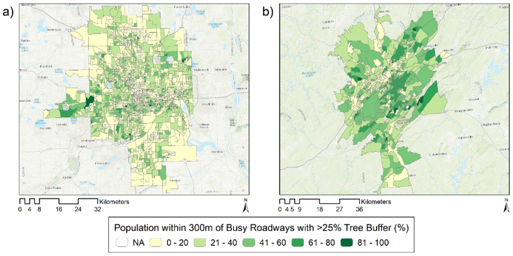
The EnviroAtlas indicator of percent residential population within 300 m of busy roadways with > 25% tree buffer relates to SDG 11.6 and is mapped here by Census block groups for areas around a) Minneapolis and St. Paul, Minnesota, and b) Birmingham, Alabama.

As previously mentioned, annual mean concentration of particulate matter of less than 2.5 microns of diameter (PM 2.5) in urban areas (μg/m3) was reported in the 2018 SDG Index and Dashboards Report for SDG 11.6.2 Annual mean levels of fine particulate matter (e.g. PM2.5 and PM10) in cities (population weighted). Although the former is a good environmental indicator of air quality for SDG 11, it falls short of the latter because it does not integrate a population component. One of the big advantages of incorporating an indicator like percent residential population within 300 m of busy roadways with > 25% tree buffer for monitoring SDG target 11.6 is the fully integrated nature of the green and gray infrastructure with the dasymetrically mapped population. When we can address biophysical and socio-economic aspects of a target in a single geospatial indicator, we may glimpse the pathways for reducing spatial inequalities. In this sense, not only are we monitoring the outcomes of a system, we are illustrating changes in infrastructure that may be altered in space and time to advance sustainable development.

The internationally agreed upon indicator SDG 4.a.1 (shown in Table 1) addresses many social and economic aspects of target SDG 4.a, yet fails to address the biophysical aspect of the learning environment. The EnviroAtlas indicator, number of K-12 schools with < 25% green space in viewshed, can contribute to evaluating whether a school facility is an inclusive and effective learning environment. Figure 8 shows the number of schools summarized to CBGs in downtown Baltimore, Maryland (Figure 8a) and the Bronx borough of New York City, New York (Figure 8b). CBGs in yellow or light green have the greatest number of K-12 schools needing additional green space to provide ecosystem services and an improved learning environment for school children.

The number of K-12 schools with < 25% green space in a 100-meter radius is another good example of an integrated indicator for both ecosystem services and SDGs. Ecosystem services supply (green space) and ecosystem services demand (school children) are incorporated into one indicator based on research of ecosystem services benefits in the scientific and public health literature. Although the incorporation of an environmental indicator from EO data may not have been considered to address this SDG target, most K-12 schools would benefit from being built or upgraded with at least 25% surrounding green space to “ensure inclusive and equitable education and promote lifelong learning opportunities for all.” Exceptions could occur for using such an indicator in national or subnational reporting where schools are in water-limited ecoregions or nations where other socio-economic priorities take precedence. This indicator currently exists only for EnviroAtlas featured communities, but available and emerging global products like Landsat and Copernicus Sentinel imagery could be used to assess the percentage of green space around georeferenced schools across the US and worldwide. Sentinel products include imagery with a 10 m resolution and a 5 day return period.

4. Discussion

EO-based indicators, like the EnviroAtlas ecosystem services indicators we have explored in this paper, are poised to help fill gaps in multi-resolution spatial, environmental, and integrated indicators in the SDG framework. Existing online geospatial portals such as EnviroAtlas that host EO-based data may be leveraged worldwide to expand the identification, creation, and use of additional SDG indicators and allow for multi-scale assessments. Given that Strengthening Actions for Nature to Achieve the Sustainable Development Goals is the selected theme of the Fifth Session of the UN Environment Assembly (UNEA-5), propounding these indicators and others like them is timely. These indicators are presented as examples of the types of SDG indicators that could be fully developed, validated, and vetted through the SDG indicator development process.

EnviroAtlas provides an example geospatial portal where decision-makers can evaluate and visualize spatial inequalities in indicators related to SDG targets. Some unique environmental and integrated indicators, where both ecosystem services supply and demand are incorporated into one indicator, have been highlighted. The percent residential population within 300 m of busy roadways with > 25% tree buffer and the number of K-12 schools with < 25% green space are two examples provided in this paper. In percent residential population within 300 m of busy roadways with > 25% tree buffer, EnviroAtlas has overcome a common integration barrier between environmental and socio-demographic data resolutions through dasymetrically mapped population that represents ecosystem services demand. Though EnviroAtlas has made great strides in utilizing EO data for evaluation of ecosystem services, we agree with Cord et al. (2017) that the full potential of EO for ecosystem services, as well as for SDGs, has yet to be realized.

As new and updated EO data become available, opportunities arise for expanding spatial extents and adding temporal resolution. The recent release of 2011 NLCD products for Alaska, Hawaiì, and Puerto Rico allows EnviroAtlas to calculate ecosystem services indicators for these locations (currently in progress). According to the Multi-Resolution Land Characteristics (MRLC) consortium, NLCD and imperviousness products are or will soon be available for 2001, 2004, 2006, 2008, 2011, 2013, and 2016 (Yang et al. 2018). The availability of comparable products across these years advances EnviroAtlas possibilities for adding temporal monitoring of ecosystem services indicators beneficial for the SDGs. If EnviroAtlas indicators are to be adopted for use in the SDG framework and subnational reporting system, another next step would be to collaborate with communities adopting SDG subnational reporting to conduct analyses and verification of proposed indicators.

With open-source/publicly available EO, geospatial data, metadata and methods, other nations may replicate these indicators and employ them for national and subnational SDG reporting. The EnviroAtlas framework, methods for indicator creation, and code are freely available for other countries to adapt for their own needs. Many of the national geospatial layers are derived from NLCD products based on Landsat data, which are also freely available around the globe. To create geospatial data layers similar to those in EnviroAtlas, nations could use one of the global land cover products derived from Landsat at 30-m resolution or from MODIS, ENVISAT MERIS, or AVHRR sensors at coarser resolutions. Data processing limitations, and periodicity of data requirements can dictate which EO product makes the most sense to use. Land cover products could then be combined with socio-economic statistics from international or national censuses, field-based observations, and other ancillary data. Although beyond the scope of this paper to investigate further, other global EO-based datasets and products that could be leveraged for indicator creation include global ecological units (Sayre et al., 2014) and Hydrosheds, a global watershed resource (Lehner et al., 2008). Additional global data can be found by searching NASA’s Global Change Master Directory (https://globalchange.nasa.gov/), the UN’s Food and Agriculture Organization’s Data Resource (http://www.fao.org/statistics/en/), and data.gov.

International censuses that can contribute socio-economic data for SDG indicators will occur in 2020 and 2030. However, the scalar disconnect between EO and socio-economic data may continue to challenge monitoring efforts for SDGs. Geographic information science offers solutions for combining datasets in transparent and robust ways to provide best-available estimates. Continued research is needed to collect and identify data and develop additional methods for creating integrated indicators for ecosystem services (Cord et al. 2015) and SDGs (Griggs et al., 2014; Scot and Rajabifard, 2017).

In addition to offering data for SDG indicators, geospatial portals offer an integrated workspace for SDG reporting where environmental, social, economic, and integrated indicators can be mapped, modeled, analyzed, and readily visualized at global, national and subnational scales/extents (Scot and Rajabifard, 2017). For proper EO and geospatial data management, we recommend following the five global statistical geospatial framework guiding principles by the United Nations Expert Group on the Integration of Statistical and Geospatial Information (outlined in Scott and Rajabifard, 2017), the priorities by Cord et al. (2017), and the proposed solutions of Lehmann et al. (2017), all found in Table 2. EnviroAtlas has been successful in following recommendations 1-4 from Scott and Rajabifard (2107); 1-2 and 4 from Cord et al. (2017); and A-C from Lehmann et al. (2017).

Table 2.

Guiding principles, priorities, and proposed solutions for managing EO-based geospatial resources for sustainable development.

Efforts	Principles/Priorities/Solutions	Reference
Guiding principles for the implementation of a global statistical-geospatial framework	1) Use of fundamental geospatial infrastructure and geocoding  2) Geocoded unit to record data in a data management environment  3) Common geographies for dissemination of statistics  4) Interoperable data and metadata standards  5) Accessible and usable geospatially enabled statistics	Scott, G. and A. Rajabifard (2017). Sustainable development and geospatial information: a strategic framework for integrating a global policy agenda into national geospatial capabilities. Geo-spatial Information Science 20(2): 59-76. (UN-GGIM 2016a) United Nations Expert Group on the Integration of Statistical and Geospatial Information
Priorities to advance monitoring of ecosystem services using earth observations	1) Defining standardized and monitorable essential ecosystem services variables  2) Advancing methods for integrating EO and socio-economic data  3) Ensuring open access, maintenance and interoperability of EO products for ecosystem services assessments  4) Utilizing EO to assess spatial disconnects between service supply and demand, trade-offs across regions and global teleconnections  5) Providing long-term opportunities for collaboration and synthesis across disciplines	Cord, A. F., et al. (2017). Priorities to Advance Monitoring of Ecosystem Services Using Earth Observation. Trends Ecol Evol 32(6): 416-428.
Proposed solutions for lowering information barriers to support sustainable development	A) Interoperability is the most important quality for improving accessibility to data, and this can be achieved through standardized protocols, data harmonization, and a sharing culture  B) Scalability is the most important quality for improving the ability to process data, and this can be achieved through grid computing  C) Openness is the most important quality for improving the ability to convey results, and this can be achieved through APIs  D) Collaboration is the most important quality for improving discussion among and between the public, scientists, and decision-makers	Lehmann, A., et al. (2017). Lifting the Information Barriers to Address Sustainability Challenges with Data from Physical Geography and Earth Observation. Sustainability 9(5): 858

Since the adoption of the 2030 Agenda and the SDGs, multiple efforts have been underway to create an international, web-based geospatial resource. The most promising product from these efforts is the Open SDG Data Hub (http://www.sdg.org/) created by Esri and the United Nations Statistics Division (UNSD). For now, the site displays maps with national SDG indicator values. The real challenge is to create an internationally agreed upon and standardized resource where both national and subnational reporting are possible. Since one of the fundamental geospatial themes of the Open SDG Data Hub is functional areas, we encourage the consideration of geopolitical and statistical boundaries, ecoregions, and watersheds, like those used by EnviroAtlas, that can be consistently mapped around the world. EO products are key for providing a source of consistent global data that can support indicator creation and aggregation to these functional areas.

Like other geospatial data and resources, EnviroAtlas was developed as a research and development (R&D) effort, and new entities may need to step up to provide long-term functionality. Online informational tools that use EO-based indicators can support national and subnational reporting efforts for the SDGs only if the tools themselves have sufficient resources to remain sustainable (Lehmann et al., 2017). Funding mechanisms to maintain infrastructure and personnel must be in place to update ecosystem services indicators with newly available EO data products for long-term monitoring and application to the SDGs.

Highlights.

• EnviroAtlas provides multi-resolution spatial indicators related to the SDGs.

• Existing EO-based data on geospatial platforms can be leveraged for SDG monitoring.

• EO-based indicators from EnviroAtlas fill gaps in environmental indicators.

• Integrated indicators are created combining land cover and demographic data.

• Addressing spatial inequalities at local levels contributes to national SDGs.

References

- Albert C, Aronson J, Fürst C, Opdam P (2014). Integrating ecosystem services in landscape planning: requirements, approaches, and impacts. Landscape Ecology, 29(8), 1277–1285. [Google Scholar]
- Aponte Clark GP, Lehner PH, Cameron DM, Frank AG (1999). Stormwater strategies: Community responses to runoff pollution. Sixth Biennial Stormwater Research & Watershed Management Conference Proceedings, 14-17 September 1999, Tampa, Florida. [Google Scholar]
- Archuleta CM, Constance EW, Arundel ST, Lowe AJ, Mantey KS, Phillips LA (2017). The National Map seamless digital elevation model specifications: U.S. Geological Survey Techniques and Methods, Book 11, Chap. B9, 39 p., 10.3133/tm11B9. [DOI] [Google Scholar]
- Armson D, Stringer P, and Ennos R (2012). The effect of tree shade and grass on surface and globe temperatures in an urban area. Urban Forestry & Urban Greening, 11(3), 245–255. [Google Scholar]
- Arnold CL, and Gibbons CJ (1996). Impervious surface coverage: the emergence of a key environmental indicator. Journal of the American Planning Association, 62, 243–258. [Google Scholar]
- Baldauf R (2017). Roadside vegetation design characteristics that can improve local, near-road air quality. Transportation Research Part D: Transport and Environment, 52, 354–361, 10.1016/j.trd.2017.03.013. [DOI] [PMC free article] [PubMed] [Google Scholar]
- Baker ME, Weller DE, Jordan TE 2006. Improved methods for quantifying potential nutrient interception by riparian buffers. Landscape Ecology, 21 (8), 1327–1345. [Google Scholar]
- Bélisle M (2005). Measuring landscape connectivity: The challenge of behavioral landscape ecology. Ecology, 86(8), 1988–1995. [Google Scholar]
- Bennett AF (2003). Linkages in the landscape: The role of corridors and connectivity in wildlife conservation. International Union for Conservation of Nature, Gland, Switzerland and Cambridge, United Kingdom: 254 p. [Google Scholar]
- Bentrup G (2008). Conservation buffers: Design guidelines for buffers, corridors, and greenways General Technical Report SRS-109, U.S. Forest Service, Southern Research Station, Asheville, North Carolina: 110 p. [Google Scholar]
- Bowler DE, Buyung-Ali L, Knight TM, Pullin AS (2010). Urban greening to cool towns and cities: A systematic review of the empirical evidence. Landscape and Urban Planning, 97, 147–155. [Google Scholar]
- Boyd J and Banzhaf S (2007). What are ecosystem services? The need for standardized environmental accounting units. Ecological economics, 63(2–3), 616–626. [Google Scholar]
- Brown C, Reyers B, Ingwall-King L, Mapendembe A, Nel J, O’Farrell P, Dixon M and Bowles-Newark NJ (2014). Measuring ecosystem services: Guidance on developing ecosystem service indicators. UNEP-WCMC, Cambridge, UK. [Google Scholar]
- Gotway CA and Young LJ (2002). Combining Incompatible Spatial Data. Journal of the American Statistical Association, 97:458, 632–648, DOI: 10.1198/016214502760047140. [DOI] [Google Scholar]
- Cord A, Seppelt R, Turner W (2015). Monitor ecosystem services from space. Nature, 523, 27–28. [DOI] [PubMed] [Google Scholar]
- Cord AF, Brauman KA, Chaplin-Kramer R, Huth A, Ziv G, Seppelt R (2017). Priorities to Advance Monitoring of Ecosystem Services Using Earth Observation. Trends Ecol Evol, 32(6), 416–428. [DOI] [PubMed] [Google Scholar]
- Curran W, and Hamilton T (2012). Just Green Enough: Contesting Environmental Gentrification in Greenpoint, Brooklyn. Local Environment, 17(9), 1027–1042. [Google Scholar]
- de Araujo Barbosa CC, Atkinson PM, Dearing JA (2015). Remote sensing of ecosystem services: A systematic review. Ecological Indicators, 52, 430–443. [Google Scholar]
- Dizdaroglu D (2017). The Role of Indicator-Based Sustainability Assessment in Policy and the Decision-Making Process: A Review and Outlook. Sustainability, 9 (6), p. 1018. [Google Scholar]
- Duque JC, Laniado H, Polo A, 2018. S-maup: Statistical test to measure the sensitivity to the modifiable areal unit problem. PLOS ONE 13 (11), e0207377. doi: 10.1371/journal.pone.0207377. [DOI] [PMC free article] [PubMed] [Google Scholar]
- Ebert DW, Wade TG (2004). Analytical Tools Interface for Landscape Assessments (ATtILA) User Manual, U.S. Environmental Protection Agency, Las Vegas, Nevada USA, 34 pp. [Google Scholar]
- Geijzendorffer IR, Cohen-Shacham E, Cord AF, Cramer W, Guerra C, Martín-López B (2017). Ecosystem services in global sustainability policies. Environmental Science & Policy, 74, 40–48. [Google Scholar]
- Giles-Corti B, Broomhall MH, Knuiman M, Collins C, Douglas K, Ng K, Lange A, Donovan RJ (2005). Increasing walking: How important is distance to, attractiveness, and size of public open space? American Journal of Preventive Medicine, 28(2, Supplement 2), 169–176. [DOI] [PubMed] [Google Scholar]
- Grêt-Regamey A, Sirén E, Brunner SH, Weibel B (2017). Review of decision support tools to operationalize the ecosystem services concept. Ecosystem Services, 26 (B), 306–315, 10.1016/j.ecoser.2016.10.012. [DOI] [Google Scholar]
- Griggs D, Smith MS, Rockström J, Öhman MC, Gaffney O, Glaser G, Kanie N, Noble I, Steffen W, Shyamsundar P (2014). An integrated framework for sustainable development goals. Ecology and Society, 19(4). [Google Scholar]
- Groffman PM, Cavender-Bares J, Bettez ND, Grove JM, Hall SJ, Heffernan JB, Hobbie SE, Larson KL, Morse JL, Neill C, Nelson K (2014). Ecological homogenization of urban USA. Front Ecol Environ, 12(1), 74–81. [Google Scholar]
- Heschong Mahone Group (2003). Windows and classrooms: Student performance and the indoor environment Technical Report P500-03-082-A-7, State of California Energy Commission, Sacramento, California. [Google Scholar]
- Hess GR, and Fischer RA (2001). Communicating clearly about conservation corridors. Landscape and Urban Planning, 55,195–208. [Google Scholar]
- Homer CG, Dewitz JA, Yang L, Jin S, Danielson P, Xian G, Coulston J, Herold ND, Wickham JD, and Megown K, 2015, Completion of the 2011 National Land Cover Database for the conterminous United States-Representing a decade of land cover change information. Photogrammetric Engineering and Remote Sensing, 81(5), 345–354 [Google Scholar]
- Jackson LE (2003). The relationship of urban design to human health and condition. Landscape and Urban Planning, 64(4), 191–200. [Google Scholar]
- Kondo MC, Fluehr JM, McKeon T, Branas CC (2018). Urban Green Space and Its Impact on Human Health. Int. J. Environ. Res. Public Health, 15(3), p. 445. [DOI] [PMC free article] [PubMed] [Google Scholar]
- Kuo F, Sullivan WC, Coley RL, Brunson L (1998). Fertile ground for community: Inner-city neighborhood common spaces. American Journal of Community Psychology, 26(6), 823–851. [Google Scholar]
- Kweon BS, Sullivan WC, Wiley AR (1998). Green common spaces and the social integration of inner-city older adults. Environment and Behavior, 30(6), 832–858. [Google Scholar]
- Lehmann A, Chaplin-Kramer R, Lacayo M, Giuliani G, Thau D, Koy K and Goldberg G (2017). Lifting the Information Barriers to Address Sustainability Challenges with Data from Physical Geography and Earth Observation. Sustainability, 9(5), p. 858 [Google Scholar]
- Lehmann I, Mathey J, Rößler S, Bräuer A, Goldberg V (2014). Urban vegetation structure types as a methodological approach for identifying ecosystem services – Application to the analysis of micro-climatic effects. Ecological Indicators, 42, 58–72. [Google Scholar]
- Lehner B, Verdin K, Jarvis A (2008). New global hydrography derived from spaceborne elevation data. Eos, Transactions, AGU, 89(10), 93–94. [Google Scholar]
- Lucci P (2015). ‘Localising’ the Post-2015 agenda: What does it mean in practice? Overseas Development Institute, London: https://www.odi.org/sites/odi.org.uk/files/odi-assets/publications-opinion-files/9395.pdf. [Google Scholar]
- Mayer PM, Reynolds SK, McCutchen MD, Canfield TJ (2006). Riparian buffer width, vegetative cover, and nitrogen removal effectiveness: A review of current science and regulations EPA/600/R-05/118. U.S. Environmental Protection Agency, Cincinnati, Ohio. [Google Scholar]
- Manickathan L, Defraeye T, Allegrini J, Derome D, Carmeliet J (2018). Parametric study of the influence of environmental factors and tree properties on the transpirative cooling effect of trees. Agricultural and Forest Meteorology, 248, 259–274. [Google Scholar]
- May CW, Horner RR, Karr JR, Mar BW, Welch EB (2003). The cumulative effects of urbanization on small streams in the Puget Sound Lowland ecoregion. University of Washington, Seattle, Washington. 26 p. [Google Scholar]
- McKay L, Bondelid T, Dewald T, Johnston J, Moore R, Rea A, (2012). NHDPlus Version 2: User Guide. U.S. Environmental Protection Agency, Washington, D.C. USA: 173 pp. [Google Scholar]
- McPherson G, Simpson JR, Peper PJ, Maco SE, Xiao Q (2005). Municipal forest benefits and costs in five US cities. Journal of Forestry, 103, 411–416. [Google Scholar]
- Millennium Ecosystem Assessment (2005). Ecosystems and Human Well-Being: Wetlands and Water Synthesis. Washington, DC, 80 pp. [Google Scholar]
- Mennis J, Hultgren T (2006). Intelligent dasymetric mapping and its application to areal interpolation. Cartography and Geographic Information Science 33(3):179–194. [Google Scholar]
- Müller F, Burkhard B (2012). The indicator side of ecosystem services. Ecosystem Services, 1 (1), 26–30, 10.1016/j.ecoser.2012.06.001 [DOI] [Google Scholar]
- NAVTEQ. NAVTEQ’s NAVSTREETS Street Data Reference Manual v4.4; NOKIA: Chicago, IL, USA, 2012. [Google Scholar]
- Neft I, Scungio M, Culver N, Singh S (2016). Simulations of aerosol filtration by vegetation: validation of existing models with available lab data and application to near-roadway scenario. Aerosol Sci. Technol, 50 (9), 937–946. [Google Scholar]
- Nowak DJ, Wang J, and Endreny T. 2007. Chapter 4: Environmental and economic benefits of preserving forests within urban areas: air and water quality Pages 28–47 in de Brun CTF (ed.), The economic benefits of land conservation. The Trust for Public Land, San Francisco, California. [Google Scholar]
- Palone RS, and Todd AH (eds.) (1997). Chesapeake Bay riparian handbook: A guide for establishing and maintaining riparian forest buffers NA-TP-02–97, U.S. Forest Service, Radnor, Pennsylvania. [Google Scholar]
- Paul MJ, and Meyer JL (2001). Streams in the urban landscape. Annual Reviews of Ecological Systems, 32, 333–365. [Google Scholar]
- Pickard BR, Daniel J, Mehaffey M, Jackson LE, Neale A (2015). EnviroAtlas: A new geospatial tool to foster ecosystem services science and resource management. Ecosystem Services, 14, 45–55. [Google Scholar]
- Pilant AN, Endres KE, Pardo S, Khopkar A, Rosenbaum D, Fizer C, Panlasigui S, Neale AC, (2016). Meter-Scale Urban Land Cover in EPA EnviroAtlas: Data, Methods and Applications for Assessing Ecosystem Services in Urban Landscapes. Presentation at American Geophysical Union Fall Meeting, Dec. 2016, San Francisco, CA. [Google Scholar]
- Sachs J, Schmidt-Traub G, Kroll C, Lafortune G, Fuller G (2018). SDG Index and Dashboards Report 2018. New York: Bertelsmann Stiftung and Sustainable Development Solutions Network (SDSN). [Google Scholar]
- Sayre R, Dangermond J, Frye C, Vaughan R, Aniello P, Breyer S, Cribbs D, Hopkins D, Nauman R, Derrenbacher W, Wright D, Brown C, Convis C, Smith J, Benson L, Paco VanSistine D, Warner H, Cress J, Danielson J, Hamann S, Cecere T, Reddy A, Burton D, Grosse A, True D, Metzger M, Hartmann J, Moosdorf N, Dürr H, Paganini M, DeFourny P, Arino O, Maynard S, Anderson M, Comer P (2014). A New Map of Global Ecological Land Units—An Ecophysiographic Stratification Approach: Washington, DC, Association of American Geographers, 46 p. [Google Scholar]
- Schueler TR (2003). Impacts of impervious cover on aquatic systems Watershed Protection Research Monograph No. 1. Center for Watershed Protection, Ellicott City, Maryland. [Google Scholar]
- Scott G and Rajabifard A (2017). Sustainable development and geospatial information: a strategic framework for integrating a global policy agenda into national geospatial capabilities. Geo-spatial Information Science, 20(2), 59–76. [Google Scholar]
- Solecki WD, Rosenzweig C, Parshall L, Pope G, Clark M, Cox J, Weinke M (2005). Mitigation of the heat island effect in urban New Jersey. Environmental Hazards, 6(1), 39–49. [Google Scholar]
- Szulczewska B, Giedych R, Borowski J, Kuchcik M, Sikorski P, Mazurkiewicz A, Stańczyk T (2014). How much green is needed for a vital neighbourhood? In search for empirical evidence. Land Use Policy, 38, 330–345. [Google Scholar]
- Tennessen CM, and Cimprich B (1995). Views to nature: Effects on attention. Journal of Environmental Psychology, 15(1), 77–85. [Google Scholar]
- Tischendorf L, and Fahrig L (2000). On the usage and measurement of landscape connectivity. Oikos, 90, 7–19. [Google Scholar]
- Ulrich RS (1981). Natural versus urban scenes. Environment and Behavior, 13(5), 523–556. [Google Scholar]
- Ulrich RS (1984). View through a window may influence recovery from surgery. Science, 224(4647), 420–421. [DOI] [PubMed] [Google Scholar]
- USDA National Agricultural Statistics Service (NASS) Cropland Data Layer. Accessed 13 September 2018, https://nassgeodata.gmu.edu/CropScape/
- US Environmental Protection Agency (EPA), EnviroAtlas One Meter Resolution Urban Land Cover Data (2008-2012) Web Service; Accessed 15 September 2018, https://edg.epa.gov/metadata/catalog/search/resource/details.page?uuid=%7Badf673a0-11b4-40d6-befd-8bf75b370cba%7D [Google Scholar]
- US Geological Survey (USGS) (2011). Gap Analysis Program (GAP), National Land Cover, Version 2.
- Vogt P, Ferrari JR, Lookingbill TR, Gardner RH, Riitters KH, Ostapowicz K (2009). Mapping functional connectivity. Ecological Indicators, 9, 64–71. [Google Scholar]
- Vogt P, Riitters K (2017). GuidosToolbox: universal digital image object analysis, European Journal of Remote Sensing, 50:1, 352–361, DOI: 10.1080/22797254.2017.1330650 [DOI] [Google Scholar]
- Wells NM (2000). At home with nature: Effects of “greenness” on children’s cognitive functioning. Environment and Behavior, 32(6), 775–795. [Google Scholar]
- Wickham J, Neale A, Mehaffey M, Jarnagin T, and Norton D, 2016. Temporal Trends in the Spatial Distribution of Impervious Cover Relative to Stream Location. Journal of the American Water Resources Association (JAWRA) 52(2): 409–419. DOI: 10.1111/1752-1688.12393 [DOI] [Google Scholar]
- Wickham JD, Wade TG, Riitters KH, Vogt P (2010). A national assessment of green infrastructure and change for the conterminous United States using morphological image processing. Landscape and Urban Planning, 94, 186–195. [Google Scholar]
- Wickham J, Stehman SV, Gass L, Dewitz JA, Sorenson DG, Granneman BJ Poss RV, Baer LA (2017). Thematic accuracy assessment of the 2011 National Land Cover Database (NLCD). Remote Sensing of Environment, 191, 328–341, DOI: 10.1016/j.rse.2016.12.026. [DOI] [PMC free article] [PubMed] [Google Scholar]
- Wolch JR, Byrne J, Newell JP (2014). Urban green space, public health, and environmental justice: The challenge of making cities ‘just green enough’. Landscape and Urban Planning, 125, 234–244. [Google Scholar]
- Wood SLR, Jones SK, Johnson JA, Brauman KA, Chaplin-Kramer R, Fremier A, Girvetz E, Gordon LJ, Kappel CV, Mandle L, Mulligan M (2018). Distilling the role of ecosystem services in the Sustainable Development Goals. Ecosystem Services, 29, 70–82. [Google Scholar]
- Wu J (2013). Landscape sustainability science: ecosystem services and human well-being in changing landscape. Landscape Ecol, 28, 999–1023. [Google Scholar]
- Xian G, Homer C, Dewitz J, Fry J, Hossain N, Wickham J (2011). The change of impervious surface area between 2001 and 2006 in the conterminous United States. Photogrammetric Engineering and Remote Sensing, 77(8): 758–762. [Google Scholar]
- Yang L, Jin S, Danielson P, Homer C, Gass L, Bender S, Case A, Costello C, Dewitz J, Fry J, Funk M, Granneman B, Liknes G, Rigge M, Xian G (2018). A new generation of the United States National Land Cover Database: Requirements, research priorities, design, and implementation strategies, ISPRS Journal of Photogrammetry and Remote Sensing, 146, 108–123. [Google Scholar]