Abstract
In this paper, we construct a stochastic model of the 2019-nCoV transmission in a confined space, which gives a detailed account of the interaction between the spreading virus and mobile individuals. Different aspects of the interaction at mesoscopic level, such as the human motion, the shedding and spreading of the virus, its contamination and invasion of the human body and the response of the human immune system, are touched upon in the model, their relative importance during the course of infection being evaluated. The model provides a bridge linking the epidemic statistics to the physiological parameters of individuals and may serve a theoretical guidance for epidemic prevention and control.
Keywords: 2019-nCoV, Stochastic model, Epidemic prevention and control, Confined space
Introduction
The novel coronavirus (2019-nCoV) was first widely known after the detection of unexplained pneumonia in the early 2020. Due to the lack of knowledge on this newly emerging virus, the 2019-nCoV began to spread rapidly and a large outbreak of the disease was globally reported. As the research goes on, a serious yet common scenario is the possibility of the aerial spreading in a relatively closed environment. Today’s world is characterized with large traffic flows at all scales. As a result, a large number of people stay in a closed space like cars, trains and airplanes often for quite long. Even if there is no contact between people, the airborne virus may still cause infection. For example, the Diamond Princess, the world’s most luxurious ocean liner, had on board more than 3700 people. A passenger was confirmed the 2019-nCoV infection on February 1st, which was followed with a total of 691 infections by the date of February 24th, with an infection rate of 18.6% [1].
With the pandemic inflicting the globe, a large number of passengers return home by air or other means of transportation. Due to the strict prevention and control measures of many governments, local traffic flows of people are restricted and residential areas become relatively isolated. According to statistics [2], humans spend 87% of their time indoors and 6% in confined microenvironments, e.g., vehicles. Therefore, living and working in a closed environment constitutes the main scene in our everyday life. Studying the dynamics of infection in a closed or semi-enclosed environment is of great significance for the ongoing and future epidemic prevention and control.
After the outbreak of the epidemic, much research [3–5] has been done to describe its development and containment, many of which are based on the susceptible–exposed–infected–removed (SEIR) compartment model, incorporating data from different temporal and spatial regions [6]. Through large-scale data analysis and extensive numerical simulation, the basic regeneration numbers of 2019-nCoV [7–10] are estimated, according to which appropriate measures may be planned and implemented for an efficient prevention and control. As a typical example, according to the latest data, Zifeng Yang [11] plotted the future development curve of the pandemic, based on an artificial intelligence (AI) approach, to estimate the parameters for large-scale simulations of phenomenological models such as the SEIR, similar to what has been done in many other works.
However, little has been done to model the viral spreading in a confined space and check how physiological specifics of individuals interact with ambient viruses. Here, we build a fully stochastic model, trying to answer some of these questions. The contamination, shedding and spreading of the virus are modeled in detail for each agent. All the stochastic simulation is done based on the Gillespie algorithm [12]. The results obtained are highly consistent with the statistics procured from the real data [13, 14].
In this study, a new model is built to simulate the dynamics of the 2019-nCoV infection in a confined space, which includes different characteristics of individuals during the transmission of 2019-nCoV and in the immune response. We estimate various parameters in our model in view of the data in news reports and published articles. Finally, by comparing results in different conditions, reasonable suggestions are made for the actual epidemic prevention and control.
Model
According to the characteristics of human infection, in the susceptibility–exposure–infection–recover (SEIR) compartment model, each individual can be in one of the five states : susceptible (S), exposed (E, infected without symptoms), hidden (H, infected without symptoms for a very long incubation period compared to the exposed), infected (I, with symptoms and infectiousness) and recover (R, never susceptible anymore). In our new model, we do not explicitly classify people into these five categories and the state of each individual is determined by two variables , being, respectively, the concentration of the 2019-nCoV in his body and the body tolerance to this virus. A person with can be regarded as a susceptible person (S). For , where is a given threshold which satisfies a uniform distribution in the interval [0, 8]; the virus carrier can be regarded as being in an incubation period (E). As the concentration of virus increases, in general, symptoms such as cough, fever, or slow movement, become more and more obvious. However, a high tolerance will exempt a person from these symptoms. As different people have different tolerances, for convenience, we assume that the tolerance to the 2019-nCoV satisfies a uniform distribution in the interval [0, 10]. We do not know how and are distributed in the crowd, so a uniform distribution is assumed in the model. However, the simulation results do not seem to depend sensitively on the exact functional form of these distributions. Since it is hard to directly measure at this time, we assume that the moving speed of a person , where m/day, such that may be used to map the tolerance. For but where T ( m/day) is another given threshold, the person is deemed to be infected (I) with symptoms (slow movement). However, for and , the person would be identified as asymptomatic (H) with no obvious symptoms. In our model, states of individuals with diverse physiological conditions are subject to dynamic changes according to their interaction with viruses in a closed environment, where spatial factors play an essential role in that the spreading of the virus and the infection of human are tightly correlated in both space and time.
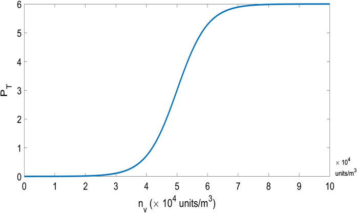
Even if a susceptible individual is exposed to the virus, he may not become infected, since a small number of viruses invading the human body can be completely degraded and eliminated by our immune system. Only when the virus concentration accumulates to a point that defies the immune system, the virus starts to proliferate exponentially. In the model, the rate of virus reproduction in the body is assumed to be sigmoidal , where is a basic production rate and z controls the steepness of the switch function. The parameter N is the previously mentioned threshold with an average value of 4. As shown in Fig. 1, when the virus concentration in the body exceeds units/m [15], the rate of virus reproduction will be greatly increased.
Fig. 1.
The rate of virus reproduction vs the virus concentration .
In the simulation, each individual will be infected with certain probability after contacting with the virus environment. Here we distinguish the virus inside the body of concentration from that on the body surface, characterized by the surface contamination degree . Each grid point (m, n) can only be occupied by at most one person and the change of the virus concentration could be described by the following reactions
where units/day is the contamination rate, is the rate at which the virus peels off into the air from the body surface and units/day is the rate of viral invasion into the human body.
Since individuals in the asymptomatic incubation period are already infectious, they can release the virus to the environment at a rate , so does the individual in state I. The changes of the virus concentration in the body and the antibody concentration secreted by immune cells are described by the reactions below
where with the basic rate, and is the rate of virus reproduction in the body. is the rate of virus being killed by antibody, and is the antibody concentration in the body, which is produced at the rate being assumed to have a uniform distribution in the interval . With the increase of virus concentration in the body, the epidemic symptoms like coughing is turning obvious, so the releasing of the virus to the environment is getting fast. However, we assume that when each infected individual releases the virus to the environment in this way, the body virus concentration does not change.
The diffusion and decay of virus concentration in the environment is modeled by the following reactions
Since the coronavirus can survive in the air for almost 3 hours [16], its decay rate is . The diffusion coefficient of virus is very weak [11]. However, due to the movement of individuals in space and sneezing to the air, the small-scale air flow increases effectively the diffusion and an effective coefficient may be set as . In total, the concentration change in a time interval is
| 1 |
where D is the virus diffusion coefficient and is the coordination number of the simulation lattice. The summation is over the adjacent lattice points.
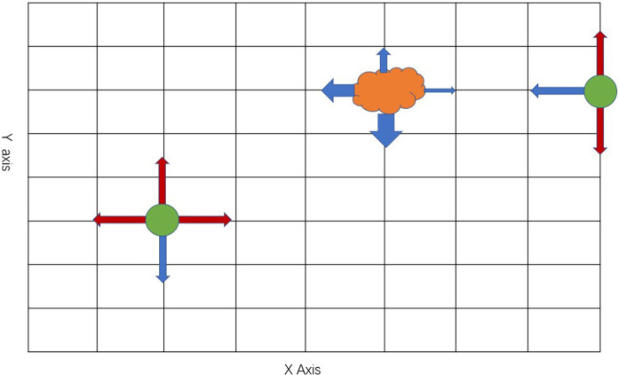
We use Gillespie algorithm to carry out the simulation of the stochastic dynamics. Information vectors are used for each individual and each grid point and get updated in each time step. The closed space is modeled as a square grid with a side length of 100 m, where the distance of adjacent grid points is 5 m. These individuals are homogeneously mixed in the space, and no attention in the model is paid to his or her own social contact network. Due to the epidemic, in a typical situation, everyone’s activities are restricted and most people spend 90% of their time in a more or less stationary state [2] and 10% in active motion. We treat each movement of an individual as a reaction. If the reaction occurs, the person can move to a randomly chosen adjacent grid point. The spreading of 2019-nCoV is a random motion in which not all viruses move together to one adjacent grid point. Only half of the viruses move to the neighboring points, such that concentration on the grid point (m, n) is reduced by half, and the other half is randomly distributed to the four adjacent grid points (Fig. 2).
Fig. 2.
Schematic representation of human movement and virus spreading: people (green circles), viruses (yellow blob), and the width of the blue arrow signals the probability of diffusion. (Color figure online)
Results
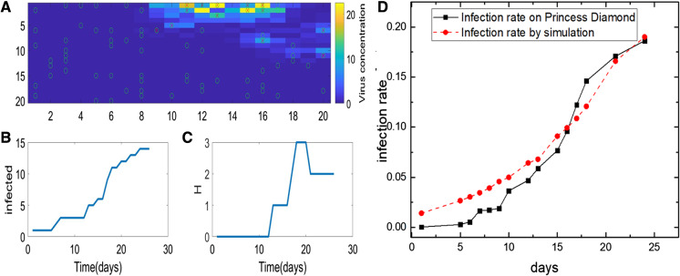
At the initial moment, we have 74 susceptible (S) individuals in a closed environment among which one is infected. The initial concentration of the virus in the infected (I) individual is . As shown in Fig. 3, after 24 days in the simulation, 14 people become infected in the confined space. The highest concentration at some grid point can reach almost . The number of people infected has been increasing over time. There are two asymptomatic infections. After averaging through multiple simulations, as shown in Fig. 3d, we display the evolution of the infection rate within 24 days, and compare it with the real data on the Diamond Princess. The curves seem to be in good agreement. The first day of the horizontal axis represents February 1, 2020, with the first confirmed case among tourists. On February 24, an average of 13.4 people were infected with the 2019-nCoV in our model, and the infection rate was 18.1%, which was basically the same as the infection rate of 18.6% on the Diamond Princess.
Fig. 3.
Plot of the simulation results. a The spatial distribution of individuals in different states, and the virus concentration in space, with the infected individual (I, red X) and the susceptible (S, green circle). The time course of the number of I (b) and H (c). d The simulated infection rate vs the real infection rate on the Princess Diamond. (Color figure online)
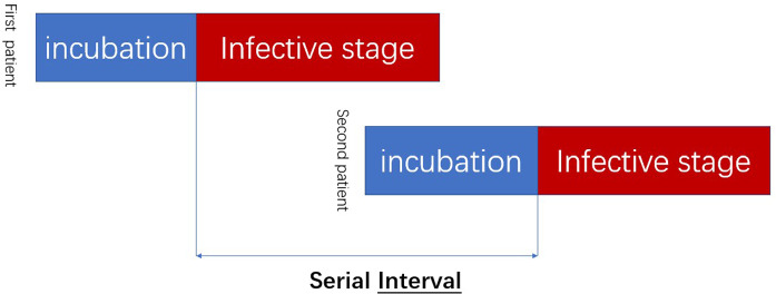
The basic reproduction number depends on the exponential growth rate of the outbreak, as well as the serial interval (SI), which is defined as the time duration between a primary and a secondary case-patient (infector) having symptom onset [17] (Fig. 4). In the model, because no epidemic prevention measures are taken, the number of infected people is growing exponentially, so we calculate the exponential growth rate as , where I(t) is the number of infected people by time t [8]. Taking the average value over a few realizations, the exponential growth rate is estimated to be 0.1081/day (the corresponding doubling time was 6.19 days). Based on the SEIR model, Joseph T Wu [7] estimated the basic regeneration number as 2.68 and the doubling time as 6.4 days; Qun Li [18] analyzed data on the first 425 confirmed cases in the early stage and found that the epidemic is doubled in size every 7.4 days with a mean serial interval of 7.5 days. According to the definition of SI, we can calculate the mean and standard deviation of the SI in our model which is considerably shorter than that of SARS (8.4 days) or MERS (14.6 days), but close to the SI estimated by Qun Li [18] and greater than the SI from the 468 confirmed cases by Zhanwei Du [19] and Nishiura [17]. Now that we have the exponential growth rate () and the SI , we can calculate the basic reproductive number of the model [20],
| 2 |
and obtain lower than previous estimates [8, 21]. If the infection threshold N of the population is uniformly distributed with a mean value of 4, the average incubation time in our model would be 4.16 days, which is the same as the one estimated by Nanshan et al [11] based on extensive on-site data. If the distribution of the infection threshold adopts an exponential form with an average value of 4, the mean incubation time obtained would be 3.08 days. Therefore, the precise distribution of the population infection threshold N is a very important factor, which can determine how quickly the virus spreads in the population.
Fig. 4.
Schematic indication of the serial interval. There are two stages for an infected person: the incubation period (blue) and the infection period (red). (Color figure online)
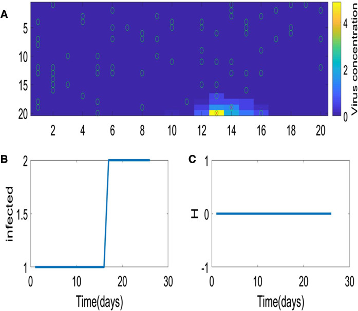
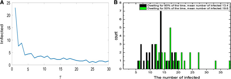
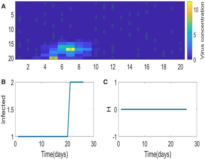
One effective way to contain the infection is to reduce the rate at which the infected individuals (I) spread the virus into the air, which cuts down the source of the virus. As shown in Fig. 5, if we change the basic rate from to , there would be only two infected person, which is hard to initiate an outbreak. It can be seen from the comparison between Figs. 3a and 5a that the highest virus concentration in the space is reduced from units/m to only about units/m. In Fig. 6a, if varies from 1 to 30, the infection rate will be greatly reduced, so limiting the amount of virus released to the environment is very effective. Another equally effective way is to reduce the contamination rate of the susceptible, as shown in Fig. 6 when is reduced from units/day to units/day. From Fig. 6b, it can also be concluded that taking measures to make people stay in their dwelling position as much as possible also helps reduce the risk of infection (Fig. 7).
Fig. 5.
The result of reducing the rate of virus release from the human body. a The spatial distribution of individuals in different states, and the distribution of virus concentration in space, with the infected (I, red X) and the susceptible (S, green circle). The time course of the number of I (b) and H (c). (Color figure online)
Fig. 6.
Influence of two different measures on the infection rate. a The number of the infected vs . b The distribution of the number of the infected with people dwelling for 90% of the time (black) and for 50% of the time (green), in 30 repeated simulation. (Color figure online)
Fig. 7.
Simulation results with . a the spatial distribution of individual in different states, and the distribution of virus concentration in space, with the infected individual (I, red X) and the susceptible (S, green circle). The time course of the number of I (b) and H (c). (Color figure online)
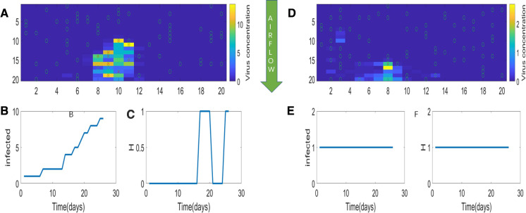
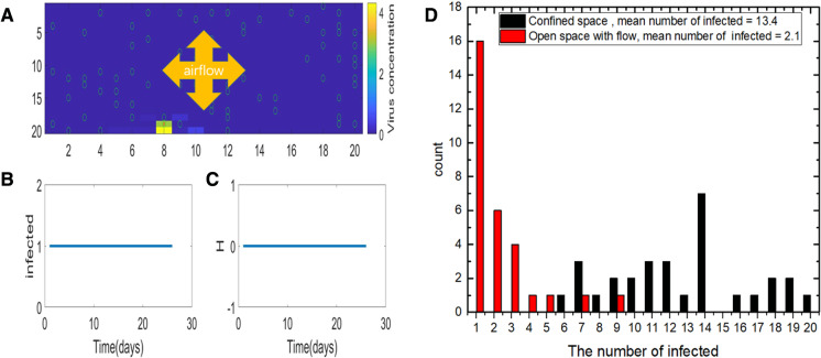
With windows being open to ventilation in this confined space, the virus will slowly float out of the boundary. In the model, we add a directional ( m/day) component to the virus velocity, aligned with the airflow. When the upper and lower boundaries of the space are open, as shown in Fig. 8, compared with the enclosed space in Fig. 3a, the virus concentration is much lower. However, in Fig. 8a, the number of infected people is not much lower than that in the enclosed space, mainly because the infected individual is in the upstream of the airflow, which exposes a lot of susceptibles to the virus. As can be seen from Fig. 8d, if instead the infected is put downstream of the airflow and next to the open boundary, the infection will decrease significantly. With all four boundaries being removed and the airflow blowing from the center, as shown in Fig. 9a, the virus is hardly concentrated. In Fig. 9d, a total of 30 simulations are conducted to find out how many people were infected 24 days later in a closed environment with the air blowing from the center. In the simulation, the initial location of the infected person is random. It is easy to see that in this condition, the number of infected people is considerably reduced when having airflow from center.
Fig. 8.
Simulation for different virus source locations. The infected individual (I) is in the center of the space (a), and at the bottom of the space (d). The airflow is blowing down. The time course of the number of I (b, e) and H (c, f)
Fig. 9.
The impact of the airflow. a The distribution of people (circles) and viruses (encoded with bar colors). The air is blowing from the center. The time course of the number of I (b) and H (c). d The distribution of the number of the infected in a confined space vs that in an open space from 30 realizations. (Color figure online)
Discussion
Through the newly constructed virus infection model, we provide useful guidance for effective prevention and control of the COVID-19 spreading, such as restricting the movement of people and placing the ventilation opening in the right position, reducing the releasing of the virus and the contact of susceptibles with unfriendly environment. All the measures will reduce the infection rate and prevent the virus from spreading to various extents. Even very simple practice such as wearing a mask could be a very effective prevention measure, especially in confined spaces. In the presence of ventilation, if the airflow is slow and only in one direction, it does not necessarily reduce the infection rate. On the contrary, it helps spread the virus and makes people downstream of the airflow more prone to viruses. To reduce the infection rate, proper arrangement of the ventilation is needed, for example, open the boundary of the space as much as possible and send fresh air from its center.
In the model, each individual has its own immunity and tolerance to the virus. We express it by the virus concentration threshold N, the virus concentration tolerance , and the human antibody growth rate . Currently, there is not enough data to take sensible statistics for these parameters and hence their exact distributions are unknown. In the current paper, a convenient form of these distributions is assumed and the plausibility is verified by comparing the simulation results with clinical data. Nevertheless, it seems that the results do not depend sensitively on the exact functional form of the distributions. It is very desirable to excavate more information from the data on these parameters.
In the future, we should start an extensive investigation of the interaction between the virus and the human immune system to microscopically compute various simulation parameters for different people to see how they are related to human genetic features. From a physicist’s point of view, it is also very interesting to construct a more realistic model to more accurately simulate different airflows from different ventilation facilities, and check the passive motion of the virus under different air conditions. Expectedly, human social networks also play a very important role in the spreading of the disease, which should be carefully considered in the study of the large-scale infection.
Acknowledgements
This work was supported by the National Natural Science Foundation of China under Grants Nos. 11775035 and 11375093, and also by the Fundamental Research Funds for the Central Universities with contract number 2019XD-A10.
Conflict of interest
The authors declare that they have no conflict of interest.
Footnotes
Publisher's Note
Springer Nature remains neutral with regard to jurisdictional claims in published maps and institutional affiliations.
Contributor Information
Zishuo Yan, Email: 13031061966@163.com.
Yueheng Lan, Email: lanyh@bupt.edu.cn.
References
- 1.What’s going on with the diamond princess? https://www.ximalaya.com/toutiao/33310347/253996510
- 2.Klepeis NE, Nelson WC, Ott WR, et al. The National Human Activity Pattern Survey (NHAPS): a resource for assessing exposure to environmental pollutants. J. Expo. Anal. Environ. Epidemiol. 2001;11(3):231–252. doi: 10.1038/sj.jea.7500165. [DOI] [PubMed] [Google Scholar]
- 3.Pastor-Satorras R, Castellano C, Van Mieghem P, et al. Epidemic processes in complex networks. Rev. Mod. Phys. 2015;87(3):925. doi: 10.1103/RevModPhys.87.925. [DOI] [Google Scholar]
- 4.Zhou Y, Ma Z. A discrete epidemic model for SARS transmission and control in China. Math. Comput. Model. 2002;40(13):1491–1506. doi: 10.1016/j.mcm.2005.01.007. [DOI] [PMC free article] [PubMed] [Google Scholar]
- 5.Ghosh, S., Samanta, G.P., Mubayi, A.: Regression approaches of survival data in the presence of competing risks: an application to COVID-19. Lett. Biomath. (2020)
- 6.He S, Tang S, Rong L. A discrete stochastic model of the COVID-19 outbreak: Forecast and control. Math. Biosci .Eng. 2020;17:2792–2804. doi: 10.3934/mbe.2020153. [DOI] [PubMed] [Google Scholar]
- 7.Wu JT, Leung K, Leung GM. Nowcasting and forecasting the potential domestic and international spread of the 2019-nCoV outbreak originating in Wuhan, China: a modelling study. Lancet. 2020;395(10225):689–697. doi: 10.1016/S0140-6736(20)30260-9. [DOI] [PMC free article] [PubMed] [Google Scholar]
- 8.Zhou T, Liu Q, Yang Z, Liao J, Yang K, Bai W, Xin L, Zhang W. Preliminary prediction of the basic reproduction number of the Wuhan novel coronavirus 2019-nCoV. J. Evid. Based Med. 2020;13:3–7. doi: 10.1111/jebm.12376. [DOI] [PMC free article] [PubMed] [Google Scholar]
- 9.Park, S.W. et al.: Reconciling early-outbreak estimates of the basic reproductive number and its uncertainty: framework and applications to the novel coronavirus (SARS-CoV-2) outbreak. MedRxiv (2020) [DOI] [PMC free article] [PubMed]
- 10.Tang B, Wang X, Li Q, et al. Estimation of the transmission risk of the 2019-nCoV and its implication for public health interventions. J. Clin. Med. 2020;9(2):462. doi: 10.3390/jcm9020462. [DOI] [PMC free article] [PubMed] [Google Scholar]
- 11.Zifeng Y, Zhiqi Z, Ke W, Sook-San W, Wenhua L, Mark Z, Peng L, Xudong C, Zhongqiang G, Zhitong M, Jingyi L, Xiaoqing L, Shiyue L, Yimin L, Feng Y, Weijie G, Yifan Y, Fei L, Shengmei L, Yuqi X, Bin L, Zhoulang W, Shaobo Z, Yaonan W, Nanshan Z, Jianxing H. Modified SEIR and AI prediction of the epidemics trend of COVID-19 in China under public health interventions. J. Thorac .Dis. 2020;12(3):165–174. doi: 10.21037/jtd.2020.02.64. [DOI] [PMC free article] [PubMed] [Google Scholar]
- 12.Gillespie DT. Exact stochastic simulation of coupled chemical reactions. J. Phys. Chem. Lett. 1977;81(25):2340–61. [Google Scholar]
- 13.Inspiration from “Diamond Princess” in science and Technology Daily: high population density and high risk of infection. https://tech.gmw.cn/2020 02/21/content_33576640.html
- 14.Real Time Updates With Credible Sources. https://coronavirus.1point3acres.com/
- 15.Shlychkov VA, Borodulin AI, Desyatkov BM, et al. Personal sampler for monitoring of viable viruses; modeling of indoor sampling conditions. Aerosol Sci. Technol. 2006;2:169–178. doi: 10.1016/j.atmosenv.2006.06.006. [DOI] [PMC free article] [PubMed] [Google Scholar]
- 16.Van Doremalen N, Bushmaker T, Morris DH, Holbrook MG, Gamble A, Williamson BN, Tamin A, Harcourt JL, Thornburg NJ, Gerber SI, Lloyd-Smith JO, de Wit E, Munster VJ. Aerosol and surface stability of SARS-CoV-2 as compared with SARS-CoV-1. New. Engl. J. Med. 2020;382(16):1564–1567. doi: 10.1056/NEJMc2004973. [DOI] [PMC free article] [PubMed] [Google Scholar]
- 17.Nishiura, H., Linton, N.M., Akhmetzhanov, A.R.: Serial interval of novel coronavirus (COVID-19) infections. Int. J. Infect. Dis. (2020) (prepublish) [DOI] [PMC free article] [PubMed]
- 18.Li Q, Guan X, Wu P, Wang X, Zhou L, Tong Y, et al. Early transmission dynamics in Wuhan, China, of novel coronavirus-infected pneumonia. N. Engl. J. Med. 2020;382(13):1199–1207. doi: 10.1056/NEJMoa2001316. [DOI] [PMC free article] [PubMed] [Google Scholar]
- 19.Du, Z., Xu, X., Wu, Y., Wang, L., Cowling, B.J., Meyers, L.A.: Serial interval of COVID-19 among publicly reported confirmed cases. Emerg. Infect. DIS. bf 26(6) (2020) [DOI] [PMC free article] [PubMed]
- 20.Wallinga J, Lipsitch M. How generation intervals shape the relationship between growth rates and reproductive numbers. Proc. Biol. Sci. 2007;274(1609):599–604. doi: 10.1098/rspb.2006.3754. [DOI] [PMC free article] [PubMed] [Google Scholar]
- 21.Zhao S, Lin Q, Ran J, Musa SS, Yang G, Wang W, Lou Y, Gao D, Yang L, He D, Wang MH. Preliminary estimation of the basic reproduction number of novel coronavirus (2019-nCoV in China, from 2019 to 2020: a data-driven analysis in the early phase of the outbreak. Int. J. Infect. Dis. 2020;92:214–217. doi: 10.1016/j.ijid.2020.01.050. [DOI] [PMC free article] [PubMed] [Google Scholar]


