The energy cost and optimal design for synchronization of coupled molecular oscillators

Abstract

A model of coupled molecular biochemical oscillators is proposed to study nonequilibrium thermodynamics of synchronization. We find that synchronization of nonequilibrium oscillators costs addition energy to drive the exchange reaction (chemical interaction) between individual oscillators. By solving the steady state of the many-body system analytically, we show that the system goes through a nonequilibrium phase transition driven by energy dissipation, and the critical energy dissipation depends on both the frequency and strength of the exchange reaction. Moreover, our study reveals the optimal design for achieving maximum synchronization with a fixed energy budget. We apply our general theory to the Kai system in Cyanobacteria circadian clock and predict a relationship between the KaiC ATPase activity and synchronization of the KaiC hexamers. The theoretical framework can be extended to study thermodynamics of collective behaviors in other extended nonequilibrium active systems.

I. INTRODUCTION

Synchronization among a population of interacting single oscillators is ubiquitous in nature [1, 2], e.g., Josephson junctions [3], circadian clocks [4], physiological rhythms [5], neurons firing [6, 7], and communication in cell populations [8, 9]. Synchronization dynamics have been well studied by using theoretical models, in particular, the Kuramoto model [10–13]. However, relatively little is known about synchronization of molecular oscillators in cellular systems where the underlying mechanism is governed by biochemical reactions with a small number of molecules and large fluctuations.

Recently, several studies were published on understanding the energetics of individual biochemical oscillators (clocks) for maintaining their phase accuracy and sensitivity [14–18]. Here, we investigate whether and how much additional energy is required to drive interaction (coupling) among individual molecular oscillators to achieve their collective behavior, i.e., synchronization. We find that exchange reactions (chemical interactions) between individual oscillators, in combination with the phase dynamics of individual oscillators, break detailed balance and thus continuous energy dissipation is needed to drive the oscillator-oscillator coupling contrary to previous thought [13, 19]. In a general model of coupled molecular clocks, we show that synchronization is achieved only when the energy dissipation reaches a critical value that depends on both the strength and frequency of oscillator-oscillator exchange reactions. Our theory further reveals the optimal choice (design) of the exchange reaction frequency and strength that leads to the maximum synchronization with a given energy budget. Finally, we apply our theory to the Kai system in the circadian clock of S. elongatus to understand its molecular mechanism for synchronization.

II. MODELS AND RESULTS

A. A model of coupled molecular clocks: the global and local dissipative cycles

We consider m interacting molecular clocks, each with N microscopic states labeled by n = 1, 2, …, N. As shown in Fig. 1A, these microscopic states can be arranged on a ring with a periodic boundary condition, i.e., state N + 1 is the same as state 1, and a phase variable ϕ ≡ n∆ϕ is defined. In this paper, we study the simple “Poisson” clock model where both the forward (clockwise) and backward (counterclockwise) transitions between two neighboring states n and n + 1 are Poisson processes with the forward rate $k_n^{+}=k$ and the backward rate $k_n^{-}=\gamma k$.

FIG. 1:

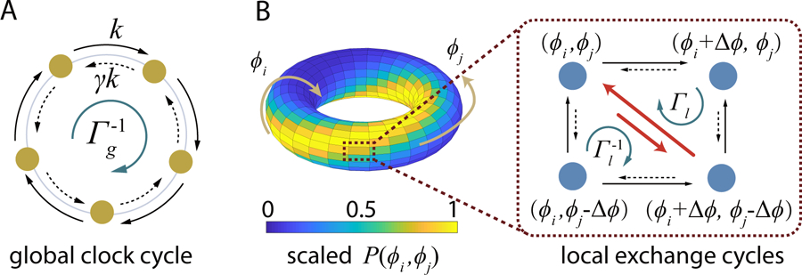
Nonequilibrium cycle dynamics of Poisson clock(s). (A) A clock steps between 2 neighboring states by Poisson processes with rates k for clockwise transitions and γk for counterclockwise transitions (γ < 1). The global clock cycle is characterized by ${\Gamma }_g={\gamma }^N$. (B) The distribution function P (ϕ_i, ϕ_j) of the phases ϕ_i and ϕ_j of two interacting Poisson clocks are shown on a torus. The transitions among 4 neighboring states in the dotted box are shown with the exchange reactions labeled by red arrows. The two local exchange cycles are characterized by ${\Gamma }_l\left(=e^{-\Delta E_{ij}}\right)$ and ${\Gamma }_l^{-1}$ with ∆E_ij the exchange reaction potential between states (ϕ_i, ϕ_j) and (ϕ_i + ∆ϕ, ϕ_j − ∆ϕ).

When $\gamma \ne 1$, detailed balance is broken as the products of reaction rates in the counterclockwise and clockwise directions in the full global clock cycle 1 → 2 → ⵈ → N → 1 become unequal as shown in Fig. 1A:

$${\Gamma }_g\equiv \prod _n{k}_n^{-}/\prod _n{k}_n^{+}={\gamma }^N\ne 1,$$ (1)

which means that time reversal symmetry is broken in the system and a sustained oscillation is possible. Driven by free energy dissipation, reactions along the ring advance the phase of the oscillator [14–16], and are thus called the processive reactions in this paper.

However, spending free energy to keep $\gamma \ne 1$ is only a necessary condition for oscillation in a single clock. Due to large fluctuations in the molecular level chemical reactions (Poisson processes), individual clocks quickly become asynchronous and macroscopic (averaged) oscillatory behavior disappears. To achieve synchronous oscillation, we introduce coupling between two individual clocks i and j as shown in Fig. 1B (red reaction arrows in the right panel). Specifically, we introduce exchange reactions between the two-clock states (ϕ_i, ϕ_j) and (ϕ_i + ∆ϕ, ϕ_j − ∆ϕ). Since the phase of an oscillator molecule (e.g., KaiC hexamer in the Kai system) is given by its chemical property such as its phosphorylation level, the total phase is conserved during the exchange reaction. The exchange reactions introduce chemical interactions between individual oscillators. These chemical interactions are different from physical interactions in the sense that they only act during the exchange reactions and they are independent of and thus do not affect the processive reactions of individual oscillators.

Without loss of generality, the forward and backward exchange reaction rates can be written as:

$$k_{ex}^{-}\left(\left({\varphi }_i+\Delta \varphi ,{\varphi }_j-\Delta \varphi \right)\to \left({\varphi }_i,{\varphi }_j\right)\right)=\frac{{\Omega }_{ij}}{m}{R}_{ij}^{-\frac{1}{2}},$$

$$k_{ex}^{+}\left(\left({\varphi }_i,{\varphi }_j\right)\to \left({\varphi }_i+\Delta \varphi ,{\varphi }_j-\Delta \varphi \right)\right)=\frac{{\Omega }_{ij}}{m}{R}_{ij}^{\frac{1}{2}},$$

where $\frac{{\Omega }_{ij}}{m}\equiv {\left[\begin{array}{cc}{k}_{ex}^{+}& k_{ex}^{-}\end{array}\right]}^{1/2}$ is the mean exchange frequency per oscillator and $R_{ij}\equiv k_{ex}^{+}/k_{ex}^{-}$ is the ratio of the two exchange reaction rates. We can define a reaction potential difference $\Delta E_{ij}\equiv \ln \left(R_{ij}\right)$. Assuming the exchange reaction rates only depend on the phase difference of the two oscillators involved, we can further express $\Delta E_{ij}=E\left({\varphi }_i-{\varphi }_j\right)-E\left({\varphi }_i-{\varphi }_j+2\Delta \varphi \right)$ where E(ϕ), a periodic function of ϕ with period 2π, characterizes the exchange reaction potential of the oscillator pair (ϕ_i, ϕ_j). For theoretical convenience, we study the case with a constant Ω_ij = Ω and a simple cosine form for E(ϕ) in this paper. Other choices of the exchange reaction rates do not change the main conclusion of this study (see SI for details).

Although the ratio of the forward and backward exchange reaction rates is written formally here as $e^{-\Delta E_{ij}}$ as in an equilibrium system, the exchange reactions cost energy in the final nonequilibrium steady state (NESS) due to the presence of the independent processive reactions of individual clocks that are not governed by ∆E_ij. This additional energy cost has an intuitive origin as we take a close look at the triangular local exchange cycle formed by the combination of two processive reactions and one exchange reaction: (ϕ_i, ϕ_j) → (ϕ_i + ∆ϕ, ϕ_j) → (ϕ_i + ∆ϕ, ϕ_j − ∆ϕ) → (ϕ_i, ϕ_j) as shown in Fig. 1B. It is easy to show the ratio of the products of the reaction rates in the clockwise and counter-clockwise directions for this local cycle is:

$${\Gamma }_l=\frac{k_{ex}^{-}}{k_{ex}^{+}}\times {\gamma }^{-1}\times \gamma =e^{-\Delta E_{ij}},$$ (2)

and ${\Gamma }_l^{-1}$ for the accompanying sister local cycle: (ϕ_i, ϕ_j) → (ϕ_i + ∆ϕ, ϕ_j − ∆ϕ) → (ϕ_i, ϕ_j − ∆ϕ) → (ϕ_i, ϕ_j). The existence of this dipole of cycles with ${\Gamma }_l\ne 1$ indicates violation of detailed balance at the local level when $\Delta E_{ij}\ne 0$ (for any oscillator pair) in addition to the global violation due to full period phase procession (Eq. 1). Since synchronization requires the exchange reactions to favor the pair of oscillators with a smaller phase difference, i.e, ∆E_ij < 0 if the pair (ϕ_i, ϕ_j) has a smaller phase difference than that of (ϕ_i + ∆ϕ, ϕ_j − ∆ϕ), Eq. 2 indicates that additional energy (in excess of those used for driving individual clocks) must be dissipated to power the exchange reactions for synchronization.

B. An analytical solution for the many-oscillator phase distribution

In the limit N → ∞, the phase of each oscillator can be described by a continuous phase variable ${\varphi }_i\equiv n_i\Delta \varphi$. By rescaling reaction rates with ∆ϕ accordingly: k(∆ϕ)² → k, Ω(∆ϕ)² → Ω, we obtain the Fokker-Planck equation for the joint distribution function of all the oscillator phases P (ϕ₁, ϕ₂, …, ϕ_m, t) :

$$\frac{\partial P}{\partial t}=k\sum _i\frac{\partial }{\partial {\varphi }_i}\left(-e_g+\frac{\partial }{\partial {\varphi }_i}\right)P+\frac{\Omega }{m}\sum _{i<j}\frac{\partial }{\partial {\phi }_{ij}}\left(2E^{\prime }\left({\phi }_{ij}\right)+\frac{\partial }{\partial {\phi }_{ij}}\right)P,$$ (3)

where φ_ij = ϕ_i − ϕ_j is the relative phase variable and ∂/∂φ_ij = ∂/∂ϕ_i − ∂/∂ϕ_j. In the continuous limit, the net speed of phase procession is ke_g with $e_g={\lim }_{N\to \infty }\ln \left({\gamma }^{-1}\right)/\Delta \varphi =-\ln {\Gamma }_g/2\pi$.

The physical meaning of the Fokker-Planck equation, Eq. 3, is clear. The first term on the right hand side (RHS) is due to the processive reactions of individual clocks, while the 2nd term on the RHS is due to the clock-clock interaction. Remarkably, the steady state distribution of the coupled many-oscillator system can be obtained analytically with a simple solution (see Methods for derivation):

$$P_s\left(\overrightarrow{\varphi }\right)=Z^{-1}\exp \left(-\beta E_t\left(\overrightarrow{\varphi }\right)\right),$$ (4)

where $E_t=\frac{2}{m}{\sum }_{\left(i<j\right)}E\left({\varphi }_i-{\varphi }_j\right)$ is the effective total interaction potential during exchange reactions, Z is the normalization constant (or the partition function), and the parameter $\beta =\frac{\Omega }{\Omega +k}$ serves as an effective inverse temperature.

It is important to point out that even though the steady state phase distribution given in Eq. 4 follows a Boltzmann distribution, the system is in a nonequilibrium steady state (NESS) with an effective nonequilibrium temperature:

$$T_{eff}={\beta }^{-1}=1+k/\Omega ,$$ (5)

which is higher than the thermal equilibrium temperature (set to unity in our study). The nonequilibrium processive reactions increase the effective temperature by k/Ω without changing the exchange interaction strength E_t.

From the steady state distribution P_s given by Eq. 4, we can compute the probability flux in the phase space of the coupled clock system. There are two types of fluxes:

$$J_i=k\left[e_g+\frac{2\beta }{m}\sum _j{E}^{\prime }\left({\phi }_{ij}\right)\right]P_s,$$ (6)

$$J_{ij}=-\frac{2\Omega }{m}\left[E^{\prime }\left({\phi }_{ij}\right)-\frac{\beta }{m}\sum _k\left(E^{\prime }\left({\phi }_{jk}\right)-E^{\prime }\left({\phi }_{jk}\right)\right)\right]P_s,$$ (7)

where J_i is the processive flux for the i-th clock; J_ij is the exchange flux between clock-i and clock-j. Both fluxes are nonzero, which means that continuous energy dissipation is needed to maintain the NESS. The free energy dissipation rate per oscillator is given by the entropy production rate [20] (see SI for derivation):

$$\dot{W}=\frac{1}{m}\int \left[\sum _i\frac{J_i^2}{k{P}_s}+\sum _{i<j}\frac{J_{ij}^2}{\frac{\Omega }{m}{P}_s}\right]d\overrightarrow{\varphi },$$ (8)

where the two terms in the RHS of Eq. 8 correspond to the dissipation for phase procession and phase exchange, respectively.

C. The energy cost for driving the nonequilibrium transition to synchronization

Following standard convention [12], we define the synchronization order parameter 0 ≤ r < 1 by

$$r{e}^{i\psi }\equiv \frac{1}{m}\sum _{j=1}^m{e}^{i{\varphi }_j},$$

where ψ is the phase of the collective oscillation. We define the phase fluctuation of oscillator i from that of the mean oscillation as:${\theta }_i\equiv {\varphi }_i-\psi$, which can be described by a distribution ρ(θ). In the asynchronous phase, ρ(θ) is uniform and r = 0; in the synchronous phase, ρ(θ) peaks at θ = 0 and r becomes finite (0 < r < 1).

For simplicity, we study a “ferromagnetic” interaction potential function $E\left({\varphi }_i-{\varphi }_j\right)=-\frac{E_0}{2}\cos \left({\varphi }_i-{\varphi }_j\right)$, with E₀(> 0) the coupling strength. By using the exact solution Eq. 4, we obtain the steady state distribution for ρ(θ) in the mean-field limit m = ∞ (see SI and Fig. S1 for simulation results for finite m):

$$\rho \left(\theta \right)=Z^{-1}\exp \left(r\beta E_0\cos \theta \right).$$ (9)

By using the above distribution function ρ(θ) in the definition for r, we obtain the self-consistent equation for the order parameter r(E₀, Ω) for any given E₀ and Ω:

$$r={\int }_0^{2\pi }\cos \theta \rho \left(\theta \right)\text{d}\theta =\frac{I_1\left(\beta E_{0}r\right)}{I_0\left(\beta E_{0}r\right)},$$ (10)

where I₀(x) and I₁(x) are the modified Bessel functions.

It can be derived from Eq. 10 (see SI for details) that the oscillators are asynchronous, i. e., r = 0 when βE₀ < 2. A phase transition to a synchronous state with r ≥ 0 occurs when βE₀ ≥ 2 or equivalently when the exchange frequency Ω is larger than a critical frequency Ω_c(E₀):

$$\Omega \ge {\Omega }_c\left(E_0\right)\equiv \frac{2k}{E_0-2}.$$ (11)

As shown in the phase diagram Fig. 2A, the synchronization transition depends on both the strength and frequency of the exchange reactions. A necessary condition for synchronization is for the exchange strength to be higher than a critical value $E_0>E_{0,c}\equiv 2$, which is analogous to the critical coupling strength in phase transitions in equilibrium systems such as the Ising model. However, this condition is not enough as synchronization also requires the exchange frequency (rate) to be larger than a critical value Ω > Ω_c(E₀). Unlike previously studied cases where nonequilibrium phase transitions are driven by varying temperature [21] or thermal force [22], this requirement for kinetic rates studied here is unique to nonequilibrium systems and has no counter part in equilibrium phase transitions.

FIG. 2:

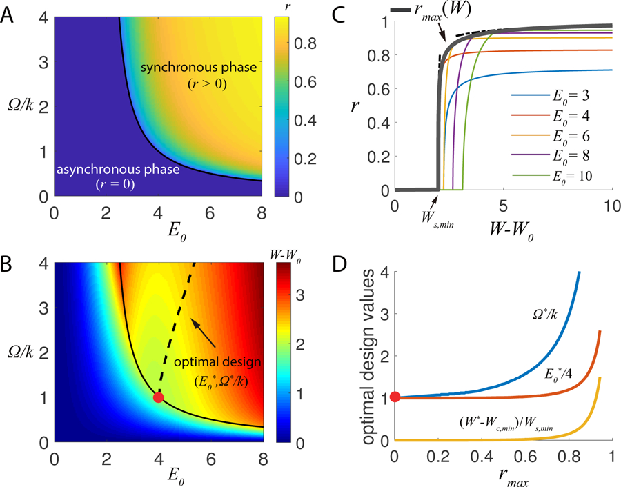
Phase diagram and optimal design for synchronization. (A) The synchronization order parameter r, and (B) the energy dissipated for the exchange reactions, W − W₀, in parameter space (E₀, Ω/k). The solid line in (A)&(B) is the phase transition line. (C) r versus the exchange energy cost (W − W₀) for different values of E₀. The thick gray line shows the envelop r_max(W), i.e., the maximum r for a given W with its asymptotic behaviors given in Eqs. (14)&(15) shown by the dotted lines. (D) The optimal choices Ω* and $E_0^{\ast }$, and the corresponding energy cost per period W* to reach the maximum performance r_max. The optimal design line $\left(E_0^{\ast },{\Omega }^{\ast }/k\right)$ is also shown in (B). Parameter e_g = 4π.

One hallmark of a nonequilibrium system is that it continuously dissipates energy even in its steady state. But what does it dissipate energy for? Here, we relate the synchronization performance characterized by its order parameter r with the free energy dissipation. By using the phase fluctuation distribution (Eq. 9) in Eq. 8, the dissipation rate per oscillator $W=\dot{W}{T}_p$ in a period T_p = 2π/(ke_g) (note that the period is independent of the exchange reactions because the total phase is preserved during an exchange reaction), can be determined analytically in the limit m → ∞:

$$W\left(E_0,\Omega \right)=W_0+\frac{2\pi \Omega \beta E_0^2}{k{e}_g}(\frac{A_2}{2\beta }-A_3),$$ (12)

where W₀ = 2πe_g is the free energy cost per period for an independent clock, $A_3\langle \sin \left({\varphi }_1-{\varphi }_2\right)\sin \left({\varphi }_1-{\varphi }_3\right)\rangle =r^2/\left(\beta E_0\right)$ and $A_2=\langle {\sin }^2\left({\varphi }_1-{\varphi }_2\right)\rangle =\frac{2}{\beta E_0}\left(1-\frac{1}{\beta E_0}\right)$ for βE₀ ≥ 2 are the two- and three-point correlation functions (see SI for derivation). The second term in the RHS of Eq.(12), $W_{ex}\left(E_0,\Omega \right)\equiv W\left(E_0,\Omega \right)-W_0$, represents the energy cost to power the exchange reactions. The dependence of W_ex on E₀ and Ω is shown in Fig. 2B.

It is clear from Eq. 12 that a finite additional energy cost is needed to increase Ω to reach the onset of synchronization at Ω = Ω_c = 2k/(E₀ − 2). This additional energy cost at the onset of collective oscillation can be defined as the synchronization energy:

$$W_s=W\left(\Omega ={\Omega }_c\right)-W_0=\frac{\pi E_0^2}{\left(E_0-2\right)e_g}.$$ (13)

Near the synchronization transition, the order parameter depends on the energy dissipation W in a power-law: $r\approx a_w{\left(W-W_c\right)}^{\frac{1}{2}}$ with a mean-field exponent 1/2 and a constant prefactor $a_w={\left[2e_g/\left(\pi E_0\right)\right]}^{\frac{1}{2}}\left(E_0-2\right)/\left|E_0-4\right|$. The critical energy cost $W_c\equiv W_0+W_s$ contains two parts, W₀ and W_s, which are responsible for the oscillation of individual clocks and their synchronization, respectively.

D. Maximizing synchronization with a ftxed energy budget

Given the dependence of r and W on Ω and E₀, we next ask what is the maximum achievable synchronization r_max(W) for a given energy budget W, and what is the optimal design of E₀ and Ω that lead to this maximum performance.

From the dependence of W_s on E₀ given by Eq. 13, there exists a minimum synchronization energy W_s,min = 8π/e_g at E₀ = 4 with the corresponding critical exchange frequency equal to the clock frequency Ω = 2k/(E₀ − 2) = k. For $W<W_{c,min}\equiv W_0+W_{s,min}$, synchronization is impossible, i.e., r_max = 0, for any coupling interaction. For W ≥ W_c,min, r_max ≥ 0, synchronization becomes possible for certain choices of E₀ and Ω.

In Fig. 2C, the dependence of r on W for different choices of E₀ are shown. The (upper) envelop of these r(W, E₀) curves defines r_max(W), which is also shown. Near the onset of synchronization $0<W/W_{c,min}-1\ll 1$, r_max follows a power law:

$$r_{max}\left(W\right)\approx c_w{\left(W-W_{c,min}\right)}^{\frac{1}{4}}$$ (14)

with a nontrivial exponent 1/4 and $c_w={\left[3e_g/\left(2\pi \right)\right]}^{\frac{1}{4}}$. For $W/W_{c,min}\gg 1$, r_max approaches 1 (perfect synchronization) with the difference (1 − r_max) inversely proportional to the energy dissipation (see SI for derivations):

$$r_{max}\left(W\right)\approx 1-\frac{\pi }{e_g\left(W-W_0\right)}.$$ (15)

The optimal choices of $E_0^{\ast }\left(W\right)$ and Ω*(W) that leads to the optimal performance for a given W are also determined. In Fig. 2D, we show the optimal exchange reactions ($E_0^{\ast }$ and Ω*) and the corresponding energy cost (W*) versus the achieved maximum synchronization r_max. For up to a modestly high level of synchronization ∼ 0.7, the optimal design for the exchange reaction is to have a roughly constant E₀ (slightly higher than 4) and to tune Ω higher for higher synchronization. This weak dependence of r_max on $E_0^{\ast }$ (as long as it is larger than a critical value) is related to the small exponent 1/4 in Eq. 14 (see Methods for a brief discussion and SI for a detailed derivation). This design for efficient synchronization is consistent with biological constraints as the reaction strength E₀ may be hard to vary in biochemical systems, but the kinetic rate Ω can be modulated by enzymes.

E. Synchronization in the Kai system

Our theoretical work is inspired by the Kai system underlying the Cyanobacteria circadian clock. The key molecules in the Kai system are the KaiC proteins that form hexamers under physiological conditions. Each KaiC monomer has two autophosphorylation sites (S-431 and T-432) in its CII domain and the different phosphorylation states of the KaiC hexamer constitute the different phases of the oscillation [23, 24]. The processive transitions between these phosphorylation states (phases) are driven by phosphorylation and dephosphorylation reactions that are controlled by two proteins, KaiA and KaiB, and by transitions between a phosphorylation (P) conformation and a dephosphorylation (dP) conformation of the hexamer [25–29]. A simple model for a single KaiC hexamer is characterized by rates of these reactions as shown in Fig. 3A (see Methods for details of the model).

FIG. 3:

The cost of monomer-shuffling for synchronization in the Kai system. (A) Scheme of single hexamer dynamics (top) and monomer shuffling between two hexamers (bottom). The red dot represents the two phosphorylation sites on each KaiC monomer. Shuffling is allowed to happen between two hexamers with the same conformation (P or dP). (B) The amplitude and period of macroscopic oscillation versus the shuffling rate R. A finite critical R, labeled by the dotted line (the same as in (C)), is required for the collective oscillation while the period (∼ 24hr) is roughly independent of R. (C) Dissipation rate per Kai monomer versus R for different values of E_s. The two gray lines correspond to the minimum energy cost per KaiC monomer for the phosphorylation-dephosphorylation cycle (2ATP/day) and the experimentally measured dissipation rate (∼ 16ATP/day), respectively. 1ATP ≈ 20k_BT is used here.

The molecular mechanism of synchronization in the Kai system is not fully understood. One possibility is the experimentally observed monomer-shuffling phenomenon that allows two KaiC hexamers to exchange monomers when the hexamers are in certain phases of their oscillation [30–35], which we focus on in this study. It is known that KaiC hexamerization requires ATP and thus it is highly plausible that ATP hydrolysis leads to KaiC hexamer disassembly [36, 37] which allows monomer-shuffling between different hexamers. Monomer-shuffling can lead to averaging of phases of the two hexamers involved, which can be described by the phase exchange reaction introduced in our coupled molecular clock model. Explicitly, for any allowed monomer-shuffling reaction H_i + H_j → H_k + H_l with i + j = k + l, where the subscript “x” is the phosphorylation level of the hexamer H_x, the reaction rate is $R\times p_{ij\to kl}$, where R is the shuffling rate per hexamer and $p_{ij\to kl}\propto \exp \left[-E_s\left(\left|k-l\right|-\left|i-j\right|\right)\right]$ with E_s(> 0) a phenomenological energy parameter. We study the effect of monomer shuffling by varying the monomer shuffling rate R. In Fig. 3B, we plot the amplitude (defined as averaged phosphorylation level) of the oscillation versus R. It is clear that synchronization, i.e., macroscopic oscillation with a non-zero amplitude appears when the shuffling rate exceeds a critical value R_c. We have also considered the cases where the shuffling rate depends on the conformational state (“P” and “dP”), which do not change the main conclusions (see SI and Fig. S2&S3 for details).

As shown in Fig. 3C, energy cost increases with the shuffling rate R and the minimum energy cost for synchronization W_s (defined the same as in Eq. 13 depends on E_s and can be bigger than the energy W₀ needed for driving oscillation of an individual hexamer. Indeed, an average of ∼ 16 ATP molecules are hydrolyzed per KaiC monomer during one period [26] while only 2 ATP molecules per KaiC are needed for the phosphorylation-dephosphorylation clock cycle for the two autophosphorylation sites in KaiC. What are the additional ATP molecules used for? It is known that they are hydrolyzed by KaiC’s ATPase activity, whose function remains a major mystery in the field. Here, our theory suggests that the KaiC ATPase activity, powered by the additional ATP molecules, may be responsible for driving synchronization in the Kai system. This additional energy cost for synchronization is not only needed for the monomer-shuffling mechanism as shown here, it also holds true for the other possible synchronization mechanism in the Kai system, i.e., the KaiA differential binding mechanism (see SI and Fig. S4&S5 for details). One immediate consequence of this general result is that a reduction in the ATPase activity will suppress any possible energy-consuming synchronization mechanism and lead to a reduced synchronization. This prediction should be tested experimentally to help reveal the underlying molecular mechanism for synchronization in the Kai system.

III. DISCUSSION

In this paper, we found that coupling mechanisms such as exchange reactions that favor the clocks with a smaller phase difference violate detailed balance and additional free energy must be spent to maintain synchronization of individual clocks. This is a general result independent of individual clock dynamics and the specific coupling mechanism. The additional energy is used to drive the coupling mechanism to correct the phase error (difference) between noisy clocks. In a simple model where individual clocks interact through exchange reactions, we showed that a finite critical amount of energy dissipation, which depends on both the frequency and the strength of the coupling mechanism, is needed to drive the non-equilibrium phase transition from a disordered (asynchronous) state to a ordered (synchronous) state. We also determined the maximum possible synchronization with a fixed energy budget as well as the optimal design of the exchange reaction for achieving the maximum synchronization efficiently.

There have been some recent studies of synchronization in simple coupled three-state-oscillator systems [38–40]. Similar to our model, these three-state-oscillator models exhibit a second-order phase transition at the onset of synchronization. However, there are two important differences. First, since the focus here is to study nonequilibrium thermodynamics in synchronization, our model is built on a thermodynamically consistent framework, which is absent in these previous studies. Second, the synchronization (coupling) mechanism directly affects the processive dynamics in these previous three-state-oscillator models, whereas they are independent reactions in our study. As a consequence, the period in these previous models varies with the coupling strength while the period is not affected by the exchange reaction strength, which is a desirable feature for biochemical oscillators. Due to the difference in oscillator-oscillator interaction, we found that synchronization is only possible in our model when the number of states in an individual oscillator N ≥ 5 (see SI and Fig. S6) whereas synchronization exists for N = 3 in these previous models.

Our theoretical results have important implications for studying biological systems. In particular, the insight on energetics of synchronization makes a previously unsuspected connection between the energy source such as the ATPase activity and the observed synchronization behavior. This connection opens up a new direction to search for possible molecular mechanisms for synchronization in specific systems such as the Kai system, which we are currently pursuing. Finally, our work provides a framework to study thermodynamics of collective behaviors in other extended nonequilibrium systems, such as the flocking dynamics [41–43], where global order arises through local interactions between active agents.

IV. METHODS

Derivation of the many-oscillator steady state phase distribution.

As the interaction potential E(ϕ_i, ϕ_j) only depends on the phase difference $\left|{\varphi }_i-{\varphi }_j\right|$, we would expect the steady state of the system to have rotational invariance, i.e. $P_s\left({\varphi }_1+\varphi ,{\varphi }_2+\varphi ,\dots ,{\varphi }_m+\varphi \right)=P_s\left({\varphi }_1,{\varphi }_2,\dots ,{\varphi }_m\right)$ for arbitrary ϕ. Consequently, we have ${\sum }_i\partial P_s/\partial {\varphi }_i=0$, which could simplify Eq.(3) to: ${\partial }_t{P}_s={\sum }_i{\partial }_{{\varphi }_i}\left[2\Omega {\sum }_{j\ne 1}{E}^{\prime }\left({\varphi }_i-{\varphi }_j\right)/m+\left(\Omega +k\right){\partial }_{{\varphi }_i}\right]P_s]=0$. The solution is $P_s\left({\varphi }_1,{\varphi }_2,\dots ,{\varphi }_m\right)=Z^{-1}\exp \left(-\beta E_t\left({\varphi }_1,{\varphi }_2,\dots ,{\varphi }_m\right)\right)$, with $\beta =\Omega /\left(\Omega +k\right)$, $E_t=\frac{2}{m}{\sum }_{i<j}E\left({\varphi }_i-{\varphi }_j\right)$, and Z the normalization constant (partition function).

The optimal design and its asymptotic behavior.

For a given energy budget W* ≥ W_c,min, the maximum possible synchronization r_max(W*) is defined by $r_{max}\left(W^{\ast }\right)\equiv {\max }_{\left(E_0,\Omega \right)\in \left\{\left(E_0,\Omega \right)|W\left(E_0,\Omega \right)=W^{\ast }\right\}}r\left(E_0,\Omega \right)$, and the corresponding optimal design values are $\left(E_0^{\ast },{\Omega }^{\ast }\right)$. Considering r increases monotonically with ΩE₀/(Ω + k), the optimal values $\left(E_0^{\ast },{\Omega }^{\ast }\right)$ are unique. $\left(E_0^{\ast },{\Omega }^{\ast }\right)$ can be determined numerically and they are plotted in Fig. 2D.

The asymptotic behavior of r_max(W) when W is near W_c,min and r_max is small can be determined as below (see SI for more details). Denoting the small deviations δE = E₀ − 4, δΩ = Ω − k and δW = W − W_c,min, in the limit of βE₀ → 2, we obtain an equation for r combining Eq.(10)&Eq.(12), from which we solve r as a function of δE and δW (neglecting higher order terms): $r\left(\delta W,\delta E\right)={\left[3e_g/\left(2\pi \right)\right]}^{\frac{1}{4}}{\left(\delta W^{\frac{1}{2}}+\delta W^{\frac{1}{2}}\delta E/2-\pi \delta W^{-\frac{1}{2}}\delta E^2/4e_g\right)}^{\frac{1}{2}}$. For a given δW, r reaches its maximum when $\delta E=e_g\delta W/\pi$. Thus we have $r_{max}\left(W\right)\approx {\left[3e_g/\left(2\pi \right)\right]}^{\frac{1}{4}}{\left(W-W_{c,min}\right)}^{\frac{1}{4}}$ as given in Eq. 14, and correspondingly $E_0^{\ast }=4+\frac{2}{3}{r}_{max}^4$ with the high power 4 given by the small exponent $\frac{1}{4}$ in Eq. 14. As a result, $E_0^{\ast }$ is insensitive to r_max(< 1) – it only increases by ∼ 8% as r_max changes from 0 to 0.7.

Details of the model for the Kai system.

As illustrated in Fig. 3A, there are two kinds of reactions: the processive reactions and monomer shuffling reactions. The processive reactions include phosphorylation, dephosphorylation, and conformational change processes. In our simplified model, a KaiC hexamer has 2 conformations: P and dP,and 7 possible phosophorylation states corresponding to the 7 possible numbers (from 0 to 6) of fully phosphorylated KaiC monomers in the hexamer. In its P-conformation, the hexamer favors the phosphorylation reactions with the forward and reverse rates for phosphorylation $\left(H_i^p\to H_{i+1}^p\right)$ given by k_p and γ₁k_p, respectively (γ₁ < 1). In its dP-conformation, the hexamer favors the dephosphorylation reactions with the forward and reverse rates for dephosphorylation $H_{i+1}^{dp}\to H_i^{dp}$ given by k_dp and γ₂k_dp, respectively (γ₂ < 1). The transitions between P and dP conformations only occur with reaction $H_6^p\to H_6^{dp}$ and $H_0^{dp}\to H_0^p$ with forward and reverse rates given by g and γ₃g, respectively (γ₃ < 1). This phosphorylation-dephosphorylation cycle (PdP cycle) and the conformational change process constitute the (global) processive cycle similar to the Poisson clock shown in Fig. 1A.

Following [35], we assume monomer shuffling happens between hexamers with the same conformation (P or dP). After shuffling, the two hexamers tend to reduce their difference of phosphorylation levels. We explicitly model this process by taking the rate of monomer shuffling reaction H_i + H_j → H_k + H_l with rate $R{p}_{ij\to kl}$, where R is the shuffling rate, and $p_{ij\to kl}=Z^{-1}\exp \left[-E_s\left(\left|k-l\right|-\left|i-j\right|\right)\right]$, with $Z={\sum }_{k,l}\exp \left[-E_s\left(\left|k-l\right|-\left|i-j\right|\right)\right]$ and E_s a phenomenological energy parameter. The reverse rate is simply $R{p}_{kl\to ij}$.

Given all these reactions, the concentration of KaiC hexamers in each state (14 states in total) is governed by a set of ordinary differential equations. From simulations of these ODEs, we can compute the amplitude and period of the collective oscillation (Fig. 3B) as well as the dissipation rate of the whole system (Fig. 3C). More technical details and parameters used for Fig. 3B&C are given in the SI.

References

- [1].Pikovsky A, Rosenblum M & Kurths J Synchronization: a universal concept in nonlinear sciences, vol. 12 (Cambridge university press, 2003). [Google Scholar]
- [2].Strogatz SH Sync: The Emerging Science of Spontaneous Order (Hyperion, 2003). [Google Scholar]
- [3].Josephson B Coupled superconductors. Reviews of Modern Physics 36, 216 (1964). [Google Scholar]
- [4].Winfree AT Biological rhythms and the behavior of populations of coupled oscillators. J. Theor. Biol 16, 15–42 (1967). [DOI] [PubMed] [Google Scholar]
- [5].Glass L Synchronization and rhythmic processes in physiology. Nature 410, 277 (2001). [DOI] [PubMed] [Google Scholar]
- [6].Pazó D & Montbrió E Low-dimensional dynamics of populations of pulse-coupled oscillators. Physical Review X 4, 011009 (2014). [Google Scholar]
- [7].Montbrió E, Pazó D & Roxin A Macroscopic description for networks of spiking neurons. Physical Review X 5, 021028 (2015). [Google Scholar]
- [8].Gregor T, Fujimoto K, Masaki N & Sawai S The onset of collective behavior in social amoebae. Science 328, 1021–1025 (2010). [DOI] [PMC free article] [PubMed] [Google Scholar]
- [9].Danino T, Mondragón-Palomino O, Tsimring L & Hasty J A synchronized quorum of genetic clocks. Nature 463, 326 (2010). [DOI] [PMC free article] [PubMed] [Google Scholar]
- [10].Kuramoto Y Self-entrainment of a population of coupled non-linear oscillators In International symposium on mathematical problems in theoretical physics, 420–422 (Springer, 1975). [Google Scholar]
- [11].Kuramoto Y Chemical Oscillations, Waves and Turbulence, vol. 19 of Springer Series in Synergetics (Springer, 1984). [Google Scholar]
- [12].Acebrón JA, Bonilla LL, Vicente CJP, Ritort F & Spigler R The kuramoto model: A simple paradigm for synchronization phenomena. Reviews of modern physics 77, 137 (2005). [Google Scholar]
- [13].Pinto PD, Penna AL & Oliveira FA Critical behavior of noise-induced phase synchronization. EPL (Europhysics Letters) 117, 50009 (2017). [Google Scholar]
- [14].Cao Y, Wang H, Ouyang Q & Tu Y The free-energy cost of accurate biochemical oscillations. Nat. Phys 11, 772–778 (2015). [DOI] [PMC free article] [PubMed] [Google Scholar]
- [15].Barato AC & Seifert U Cost and precision of brownian clocks. Phys. Rev. X 6, 041053 (2016). [Google Scholar]
- [16].Barato AC & Seifert U Coherence of biochemical oscillations is bounded by driving force and network topology. Phys. Rev. E 95, 062409 (2017). [DOI] [PubMed] [Google Scholar]
- [17].Gingrich TR & Horowitz JM Fundamental bounds on first passage time fluctuations for currents. Physical review letters 119, 170601 (2017). [DOI] [PubMed] [Google Scholar]
- [18].Fei C, Cao Y, Ouyang Q & Tu Y Design principles for enhancing phase sensitivity and suppressing phase fluctuations simultaneously in biochemical oscillatory systems. Nature communications 9, 1434 (2018). [DOI] [PMC free article] [PubMed] [Google Scholar]
- [19].Lee S, Hyeon C & Jo J Thermodynamic uncertainty relation of interacting oscillators in synchrony. Phys. Rev. E 98, 032119 (2018). [Google Scholar]
- [20].Lan G, Sartori P, Neumann S, Sourjik V & Tu Y The energy–speed–accuracy trade-off in sensory adaptation. Nat. Phys 8, 4228 (2012). [DOI] [PMC free article] [PubMed] [Google Scholar]
- [21].Herpich T, Thingna J & Esposito M Collective power: Minimal model for thermodynamics of nonequilibrium phase transitions. Physical Review X 8, 031056 (2018). [Google Scholar]
- [22].Nguyen B, Seifert U & Barato AC Phase transition in thermodynamically consistent biochemical oscillators. The Journal of Chemical Physics 149, 045101 (2018). [DOI] [PubMed] [Google Scholar]
- [23].Nakajima M et al. Reconstitution of circadian oscillation of cyanobacterial kaic phosphorylation in vitro. Science 308, 414–415 (2005). [DOI] [PubMed] [Google Scholar]
- [24].Rust MJ, Markson JS, Lane WS, Fisher DS & O’shea EK Ordered phosphorylation governs oscillation of a three-protein circadian clock. Science 318, 809–812 (2007). [DOI] [PMC free article] [PubMed] [Google Scholar]
- [25].van Zon JS, Lubensky DK, Altena PR & ten Wolde PR An allosteric model of circadian kaic phosphorylation. Proceedings of the National Academy of Sciences 104, 7420–7425 (2007). [DOI] [PMC free article] [PubMed] [Google Scholar]
- [26].Terauchi K et al. Atpase activity of kaic determines the basic timing for circadian clock of cyanobacteria. Proceedings of the National Academy of Sciences 104, 16377–16381 (2007). [DOI] [PMC free article] [PubMed] [Google Scholar]
- [27].Lin J, Chew J, Chockanathan U & Rust MJ Mixtures of opposing phosphorylations within hexamers precisely time feedback in the cyanobacterial circadian clock. Proceedings of the National Academy of Sciences 111, E3937–E3945 (2014). [DOI] [PMC free article] [PubMed] [Google Scholar]
- [28].Abe J et al. Atomic-scale origins of slowness in the cyanobacterial circadian clock. Science 349, 312–316 (2015). [DOI] [PubMed] [Google Scholar]
- [29].Chang Y-G et al. A protein fold switch joins the circadian oscillator to clock output in cyanobacteria. Science 1260031 (2015). [DOI] [PMC free article] [PubMed] [Google Scholar]
- [30].Kageyama H et al. Cyanobacterial circadian pacemaker: Kai protein complex dynamics in the kaic phosphorylation cycle in vitro. Molecular cell 23, 161–171 (2006). [DOI] [PubMed] [Google Scholar]
- [31].Emberly E & Wingreen NS Hourglass model for a protein-based circadian oscillator. Physical review letters 96, 038303 (2006). [DOI] [PMC free article] [PubMed] [Google Scholar]
- [32].Ito H et al. Autonomous synchronization of the circadian kaic phosphorylation rhythm. Nature structural & molecular biology 14, 1084–1088 (2007). [DOI] [PubMed] [Google Scholar]
- [33].Mori T et al. Elucidating the ticking of an in vitro circadian clockwork. PLoS biology 5, e93 (2007). [DOI] [PMC free article] [PubMed] [Google Scholar]
- [34].Yoda M, Eguchi K, Terada TP & Sasai M Monomer-shuffling and allosteric transition in kaic circadian oscillation. PloS one 2, e408 (2007). [DOI] [PMC free article] [PubMed] [Google Scholar]
- [35].Eguchi K, Yoda M, Terada TP & Sasai M Mechanism of robust circadian oscillation of kaic phosphorylation in vitro. Biophysical journal 95, 1773–1784 (2008). [DOI] [PMC free article] [PubMed] [Google Scholar]
- [36].Mori T et al. Circadian clock protein kaic forms atp-dependent hexameric rings and binds dna. Proceedings of the National Academy of Sciences 99, 17203–17208 (2002). [DOI] [PMC free article] [PubMed] [Google Scholar]
- [37].Akiyama S Structural and dynamic aspects of protein clocks: how can they be so slow and stable? Cellular and Molecular Life Sciences 69, 2147–2160 (2012). [DOI] [PMC free article] [PubMed] [Google Scholar]
- [38].Prager T, Naundorf B & Schimansky-Geier L Coupled three-state oscillators. Physica A: Statistical Mechanics and its Applications 325, 176–185 (2003). [Google Scholar]
- [39].Wood K, Van den Broeck C, Kawai R & Lindenberg K Continuous and discontinuous phase transitions and partial synchronization in stochastic three-state oscillators. Physical Review E 76, 041132 (2007). [DOI] [PubMed] [Google Scholar]
- [40].Assis VR, Copelli M & Dickman R An infinite-period phase transition versus nucleation in a stochastic model of collective oscillations. Journal of Statistical Mechanics: Theory and Experiment 2011, P09023 (2011). [Google Scholar]
- [41].Vicsek T, Czirók A, Ben-Jacob E, Cohen I & Shochet O Novel type of phase transition in a system of self-driven particles. Physical review letters 75, 1226 (1995). [DOI] [PubMed] [Google Scholar]
- [42].Toner J & Tu Y Flocks, herds, and schools: A quantitative theory of flocking. Physical review E 58, 4828 (1998). [Google Scholar]
- [43].Toner J & Tu Y Long-range order in a two-dimensional dynamical xy model: how birds fly together. Physical review letters 75, 4326 (1995). [DOI] [PubMed] [Google Scholar]
Associated Data
This section collects any data citations, data availability statements, or supplementary materials included in this article.