Abstract
The latest Coronavirus (COVID-19) has become an infectious disease that causes millions of people to infect. Effective short-term prediction models are designed to estimate the number of possible events. The data obtained from 30th January to 26 April, 2020 and from 27th April 2020 to 11th May 2020 as modelling and forecasting samples, respectively. Spatial distribution of disease risk analysis is carried out using weighted overlay analysis in GIS platform. The epidemiologic pattern in the prevalence and incidence of COVID-2019 is forecasted with the Autoregressive Integrated Moving Average (ARIMA). We assessed cumulative confirmation cases COVID-19 in Indian states with a high daily incidence in the task of time-series forecasting. Such efficiency metrics such as an index of increasing results, mean absolute error (MAE), and a root mean square error (RMSE) are the out-of-samples for the prediction precision of model. Results shows west and south of Indian district are highly vulnerable for COVID-2019. The accuracy of ARIMA models in forecasting future epidemic of COVID-2019 proved the effectiveness in epidemiological surveillance. For more in-depth studies, our analysis may serve as a guide for understanding risk attitudes and social media interactions across countries.
Keywords: COVID-19, Spatio-temporal analysis, Weighted overlay, ARIMA, Disease forecasting
Introduction
Coronaviruses (CoV), which are the major source of diseases ranging from mild colds to more acute diseases such as Middle East Respiratory Syndrome (MERS-CoV) and Severe Acute Respiratory Syndrome (SARS-CoV), according to the World Health Organisation (WHO 2020). A new coronavirus (nCoV) is a new strain not identified in humans in the past. Infections are usually seen as signs of the skin, fever, cough, shortness of breath and trouble breathing. In more serious cases, influenza, severe acute respiratory syndrome, organ failure, or even death may be caused by infection (Sohrabi et al. 2020).
Surveillance and early notice were important for the prevention of infectious disease outbreaks. Therefore, developing epidemiological models and making forecasts are useful for the prevention and management of COVID-19. Due to their impact on the public health system, the prediction of diseases is important as accurate as possible. AI models are commonly used to forecast epidemiological time series over the years to ensure this accuracy (Davis et al. 2019). Autoregressive Integrated Moving Average (ARIMA) models are time domain tools of time-series analysis which have been extensively used of infectious diseases forecasting (Liu et al. 2011; Zeng et al. 2016).
To assess, interpret and respond to any disease epidemic, especially in pandemics like coronavirus 2019 (COVID-19), geographical knowledge is important (Murugesan et al. 2020). To identify the sources of the outbreaks, their distribution trend and their severity and take precautions, preventative steps and tracking steps, Geographic Information System (GIS) allows epidemiologists and chart epidemic incidents across various criteria, including population, the climate, geographies, historical occurrences. To recognize at-risk communities in real-time epidemic models and prepare tailored initiatives, such as evaluating existing services or developing capacity for healthcare, GIS public authorities, policymakers and managers need GIS (Boulos 2004). Furthermore, good contact with other assisting organizations and people is required to ensure a cohesive response. Time-enabled maps demonstrate how pathogens propagate over time and where health planners or administrators may want to go for action. COVID-19 has adverse impacts on other demographic groups, such as the elderly and the underlying health problems (Zhou et al. 2020). The detection of social gaps, age and other variables help you track target categories and serving areas. Current and potential impacts of COVID-19 can be understood and addressed via map, employees or citizens, medical resources, equipment, goods and services.
In this context, the purpose of this article is to explore and compare predictive potential in the sense of cumulative weekly forecasting COVID-19 cases in India using machine learning regression and statistical models. In addition, we analysed the spatio-temporal pattern of COVID-19 distribution at regional level.
Materials and methods
Data collection and integration into GIS database
The data collected relates to the total reported cases of COVID-19 in India between 30th January and 26 April, 2020. The dataset was obtained from the application programming interface (https://www.covid19india.org/), which gathers, extracts and publishes daily information from all 28 Indian State Health Offices about COVID-19 events. Excel 2013 is used to build a time-series database. The dataset was split into two areas: a training set and a test set. The training range for model design was observed from 30th January to 26 April, 2020 and testing tests were carried out from 27th April 2020 to 11th May 2020. The district boundary of India is collected from http://www.covid19india.org. The raw file is converted into shapefile in QGIS software version 3.0 and topological error has been removed. The shapefile is registered into Universal Transverse Mercator (UTM) projection and World Geodetic System (WGS) 84 datum. Total number of confirmed cases, deaths and restorations are recorded every day and arrange into Microsoft excel. After that, districtwise epidemiological data is integrated into GIS layer for further analysis. Moreover, total number of population and population density of each district is collected separately and integrated into GIS layer. Subsequently, incidence rate is calculated for each district. Alternatively, regional status (metropolitan, sub-urban, satellite town and others) of each district is collected and integrated into GIS database.
Spatial analysis
Spatial distribution of COVID-19 outbreak has been analysed at district level by considering number of cases (as on 09th May, 2020), population density, and regional status of 734 districts of India. The above parameters are analysed in GIS environment. Each aspect is divided into five categories based on the geometric interval and the weightages are assigned into four categories as (i) 4 for ‘very high risk’, (ii) 3 for ‘high risk’, (iii) 2 as ‘medium risk’, and (iv) 1 as ‘low risk’. Finally, weightage overlay analysis is performed to demarcated COVID-2019 risk zone of India.
ARIMA model
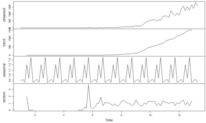
The ARIMA model comprises the Autoregressive (AR) model and Moving Average (MA) with integration based on the decomposition method (Fig. 1). ARMA model is a mixture of AR and MA models, in which all current and historical residual series values in the present time series are expressed linearly (Zhang et al. 2014). This is as follows:
Fig. 1.
Decomposition of Multiplicative time-series data and ARIMA forecast graph for 2019-nCoV prevalence. From top to bottom, the lines represent actual observations, the trend, seasonal, and random components
The ARIMA model is usually referred to as ARIMA (p, d, q) × (P, D, Q)S. P is the seasonal order of autoregressive, p is the non-seasonal order of autoregressive, Q is the seasonal moving average, q is the non-seasonal moving average order, d is the order of regular differentiation and D is the order of seasonal differentiation. The letter “s” in the subscription shows the seasonal period. In the present analysis, for instance, the occurrence of infectious diseases varies over the weekly period, s = 7. In the present study auto ARIMA has used to forecast COVID-19 outbreak.
The ADF (Augmented Dickey–Fuller) has performed to check either the data is stationary or not, as well as log transformation and differences were calculated to stabilize the time-series data (Cheung and Lai 1995). The data has no seasonal effects; therefore, it has considered as non-seasonal stationary data. Although, in the present study auto ARIMA has used to select p, d, q values to define model order, where ARIMA (2, 2, 2) has been considered as best fit, hence the order has taken to forecast.
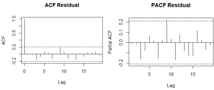
Auto-correlation function (ACF) graph and partial auto-correlation (PACF) correlogram were calculated for the ARIMA model parameters (Fig. 2). ACF helps the researchers to classify knowledge related to the concurrent finding in the previous time. The partial ACF (PACF) is used to calculate the degree of interaction between observation and observation made within two intervals of the time of elimination. PACF helps to determine with its preceding values the correctness degree of current variables while retaining certain constant values (Makridakis et al. 1998). Stationary data, along with ACF and PACF, are considered over time. Time diagram shows that the data are distributed in a horizontal way, the ACF and PACF values decline fairly fast close to zero.
Fig. 2.
Auto-correlation function (ACF) graph and partial auto-correlation (PACF) correlogram
Data validation
To assess the efficacy of the two prediction methods used in this study, contrasts between the raw series observed and the predicted values obtained through the two methods were compared. The mean absolute error (MAE) and Root mean square error (RMSE) have been chosen as measurements, since the combined and chosen estimates for calculating bias and model accuracy as analytical methods have been used widely (Christodoulos et al. 2011):
where Pt is the predicted value at time t, Zt is the observed value at time t and T is the number of predictions.
Where n is the number of observations, yi and the ith values, respectively, are measured and predicted. The Mc and Mb also represent the measurement of the performance of comparative and best models.
Results and discussion
During the period between 30th January and 26th April 2020, 62,865 number of COVID cases have been recorded and 2101 number of deaths is reported. Out of 734 districts, 188 districts have no COVID case and 48 districts have single number of cases. Mumbai District in Maharashtra is recorded the highest number of cases (14,521), followed by Gujrat district in Ahmedabad (6086), Tamilnadu in Chennai (4372) and Pune in Maharashtra (2789). Based on the incidence rate, India is divided into 6 classes, namely (i) no cases (48 districts) (ii) 1–10 (221 districts), (iii) 11–25 (91 districts), (iv) 26–50 (86 districts), (v) 51–100 (62 districts) and (vi) more than 101 (85). The maximum number of cases is considered as high risk for disease transmission and vice versa. Based on the population density, the district is classified as (i) less than 100 (122 districts), (ii) 101–250 (158 districts), (iii) 251–500 (178 districts), (iv) 501–1000 (161 districts) and (v) more than 1000 (115 districts). In this analysis, the maximum population density is considered for high risk of CoV and vice versa (Table 1). By considering urbanization pattern and movement of population, India is divided into 4 major categories, such as (i) metropolitan (22 districts), (ii) sub-urban (38 districts), (iii) satellite town (13 districts) and (iv) others (661 districts).
Table 1.
Weighted overlay analysis for COVID-19
| Parameter | Sub-parameter | Rank | Weighted value |
|---|---|---|---|
| Confirmed case (number) | < 1 | 0 | 50% |
| 1–10 | 1 | ||
| 11–25 | 2 | ||
| 26–50 | 3 | ||
| 51–100 | 4 | ||
| > 100 | 5 | ||
| Population density (Pop/sq km) | < 100 | 1 | 25% |
| 101–250 | 2 | ||
| 251–500 | 3 | ||
| 501–1000 | 4 | ||
| > 1000 | 5 | ||
| Regional status | Metro | 5 | 25% |
| Sub-urban | 4 | ||
| Non-metro | 3 | ||
| Others | 2 |
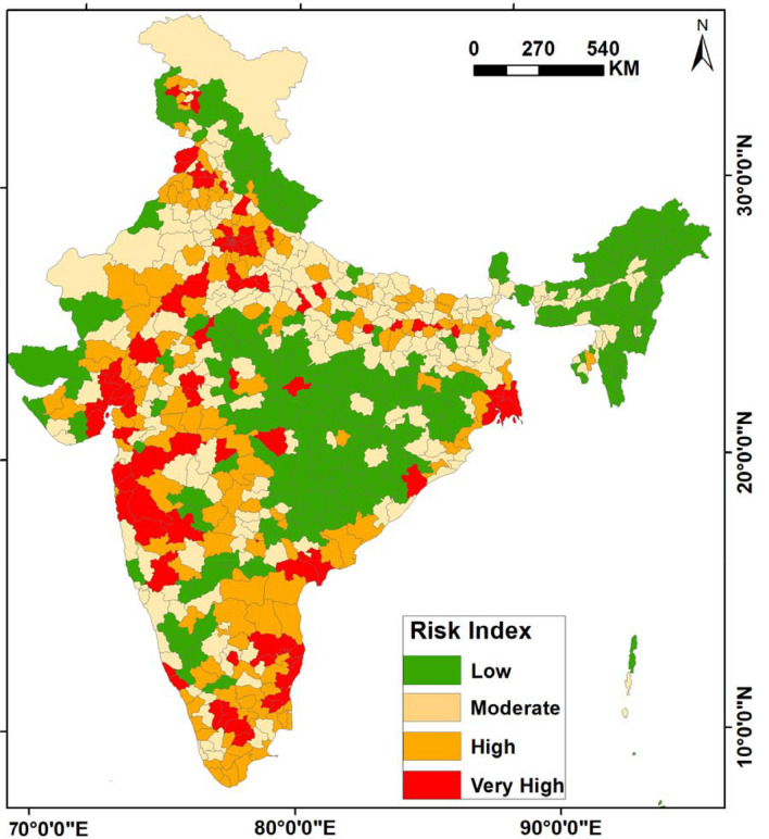
Based on the weighted overlay analysis, the district is classified into four major categories (i) less than 1.25 (257 districts), (ii) 1.26–2.25 (225 districts), (iii) 2.26–3.25 (154 districts), and (iv) more than 3.26 (98 districts) (Fig. 3). Results also showed most of the ‘low risk zone’ are distributed in central-east, north-east and small pockets of north in India. The high-risk zone is distributed in the west, south, south-west and central-north districts of India. Remaining districts are considered as moderate risk zone for COVID-19.
Fig. 3.
Spatial distribution of COVID-2019 risk zone in India (during the period between 26th January and 09th May 2020)
ARIMA models are fitted to the COVID-2019 diseases from 26th January 2020 to 09th May 2020. Table 1 presents the results of the estimations using ARIMA processes for the COVID-2019 diseases incidence time series. The selections of the best model are performed according to the principle of AIC and BIC. Descriptive data analyses were carried out to determine the occurrence of the latest COVID-2019 reported cases and to avoid potential prejudices. The ACF and PACF correlogram revealed that both the prevalence and the occurrence of COVID-2019 had no seasonality impact (Benvenuto et al. 2020). Results present the projections of incidence data with relative confidence intervals of 95%.
Table 2 indicates a rising tendency towards the peak of epidemics as a whole due to prevalence of COVID-2019. The incidence exhibited an increasing short-term trend during these 3 month period. The disparity between 1-day cases and (Xn – Xn − 1) cases of the previous day showed that the number of confirmed cases was constantly rising. Moreover, a distinct seasonality pattern is also exhibited.
Table 2.
ARIMA p, d, q (2, 2, 2) model parameter for COVID-19 forecasting
| AR1 | AR2 | MA1 | MA2 | AIC | AICc | BIC | |
|---|---|---|---|---|---|---|---|
| Co-efficient | 0.0276 | 0.2439 | − 1.8344 | 0.8818 | 1032.94 | 1033.7 | 1045.16 |
| Standard error | 0.1303 | 0.1289 | 0.0713 | 0.0675 |
Although further data are needed for a more detailed prediction, the dissemination of the virus seems to decrease significantly. Furthermore, the frequency is marginally decreased, although the number of confirmed cases continues to rise. The number of cases will hit a peak if the virus does not produce new mutations (Fig. 4).
Fig. 4.
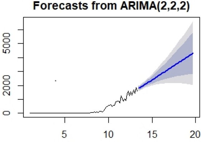
Correlogram and ARIMA forecast graph for the 2019-nCoV incidence
The prediction and estimation obtained depend on the “event” description and data collection modality. Case definition and data collection must be maintained in real time for further comparisons or for future perspectives. Generally, the fitting values and predicted values obtained by two methods (MAE, MASE) reasonably matched the real incidence of the COVID-2019 diseases. The standard errors of the MAE and RMSE are quite small, indicating that these MAE and RMSE index values are quite stable (Table 3).
Table 3.
Statewise prediction at 95% confidence level (major outbreaks has considered)
| Name of the state | 03-05-2020 | 10-05-2020 | 17-05-2020 | 24-05-2020 | 31-05-2020 | 06-06-2020 |
|---|---|---|---|---|---|---|
| Maharashtra | 15,329 | 23,084 | 31,918 | 41,794 | 52,651 | 64,456 |
| Gujrat | 6479 | 10,072 | 14,182 | 18,719 | 23,627 | 28,869 |
| Madhya Pradesh | 4405 | 7131 | 10,304 | 13,845 | 17,706 | 21,855 |
| Delhi | 5117 | 7223 | 9503 | 11,957 | 14,585 | 17,385 |
| Rajasthan | 3527 | 5021 | 6719 | 8585 | 10,596 | 12,739 |
| Tamilnadu | 2959 | 4181 | 5591 | 7158 | 8861 | 10,688 |
| Uttar Pradesh | 2869 | 3857 | 4955 | 6162 | 7478 | 8904 |
| Andhra Pradesh | 1666 | 2251 | 2912 | 3650 | 4464 | 5354 |
| West Bengal | 1181 | 1780 | 2464 | 3232 | 4081 | 5012 |
| Karnataka | 770 | 1152 | 1628 | 2182 | 2803 | 3485 |
| Bihar | 653 | 1020 | 1416 | 1839 | 2285 | 2753 |
| Jammu and Kashmir | 788 | 1052 | 1344 | 1665 | 2016 | 2396 |
| Telangana | 1175 | 1326 | 1477 | 1627 | 1778 | 1929 |
| Punjab | 522 | 712 | 914 | 1126 | 1349 | 1582 |
| Haryana | 469 | 638 | 813 | 992 | 1175 | 1361 |
| Kerala | 525 | 574 | 623 | 672 | 721 | 771 |
| Orissa | 202 | 292 | 385 | 479 | 576 | 674 |
MAE measures the average magnitude of errors in forecast sets, without considering their direction. The RMSE (95.322) always should be grater or equal to MAE (50.109), more difference between them indicates more individual errors in the variance (Fig. 5).
Fig. 5.
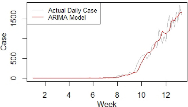
Time-series graph with ARIMA model for the 2019-nCoV incidence
Late epidemic behaviour identification is important for monitoring and preventing infectious diseases. The effectiveness of predictive models in predicted incidences of infectious disease has proven useful (Zhang et al. 2014). Figure 6 shows the modelling and predictions performances of ARIMA model. Generally, the fitting values and predicted values obtained by this analysis are matched the real incidence of COVID-19. Table 2 shows the weekly predicted values of COVID-2019 of major outbreaks state of India during the period between 03rd May 2020 and 07th June 2020. Prediction has been done for the 18 states of India which are worstly affected by COVID-19. Results showed maximum number of cases are recorded from Maharashtra state, followed by Gujrat, Madhya Pradesh and Delhi.
Fig. 6.
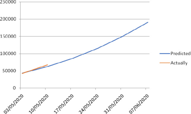
Forecasting at 95% confidence level COVID-2019 cases based on the daily incidence report using ARIMA model
Conclusion
In the present study, we conducted an experimental study in the forecasting of the COVID-2019 epidemic pattern and have also compared the differences of actual and predicted values in both principle and practical aspects. Moreover, the based on weighted overlay, the district are classified into very high, high, medium and low risk zone of COVID-2019. The ARIMA model can acquire (1) AR for considering past values and (2) MA to consider current and preceding residual series historical knowledge. An efficient linear model to efficiently capture a linear pattern of the COVID-19 disease series was demonstrated in the ARIMA model. In general, decomposition methods operate best when the sequence is compatible with the hypothesis for decomposition. The drawback of the model is that only the data from the time series can derive linear relationships. With events which may be influenced by multiple factors, including several meteorological and specific social influences, this does not work well. When used on other cases, the findings based on a particular disease may not be repeatable. Moreover, there are several other theories about the long-term trend in methods of decomposition, such as generalized models and Support Vector Machine (SVM), which assume a nonlinear function in the time series.
Compliance with ethical standards
Conflict of interest
There is no conflict of interest between the authors.
Footnotes
Publisher's Note
Springer Nature remains neutral with regard to jurisdictional claims in published maps and institutional affiliations.
Contributor Information
Santanu Roy, Email: roysantanu.rs@gmail.com.
Gouri Sankar Bhunia, Email: rsgis6gouri@gmail.com.
Pravat Kumar Shit, Email: pravatgeo2007@gmail.com.
References
- Benvenuto D, Giovanetti M, Vassallo L, Angeletti S, Ciccozzi M. Application of the ARIMA model on the COVID-2019 epidemic dataset. Data Brief. 2020;29:105340. doi: 10.1016/j.dib.2020.105340. [DOI] [PMC free article] [PubMed] [Google Scholar]
- Boulos MNK. Towards evidence-based, GIS-driven national spatial health information infrastructure and surveillance services in the United Kingdom. Int J Health Geogr. 2004 doi: 10.1186/1476-072X-3-1. [DOI] [PMC free article] [PubMed] [Google Scholar]
- Cheung Y-W, Lai KS. Lag order and critical values of the augmented Dickey–Fuller test. J Bus Econ Stat. 1995;13:277–280. [Google Scholar]
- Christodoulos C, Michalakelis C, Varoutas D. On the combination of exponential smoothing and diffusion forecasts: an application to broadband diffusion in the OECD area. Technol Forecast Soc Change. 2011;78:163–170. doi: 10.1016/j.techfore.2010.08.007. [DOI] [Google Scholar]
- Davis JK, Gebrehiwot T, Worku M, Awoke W, Mihretie A, Nekorchuk D, et al. A genetic algorithm for identifying spatially-varying environmental drivers in a malaria time series model. Environ Model Softw. 2019;119:275–284. doi: 10.1016/j.envsoft.2019.06.010. [DOI] [PMC free article] [PubMed] [Google Scholar]
- Liu Q, Liu X, Jiang B, Yang W. Forecasting incidence of hemorrhagic fever with renal syndrome in China using ARIMA model. BMC Infect Dis. 2011;11:218. doi: 10.1186/1471-2334-11-218. [DOI] [PMC free article] [PubMed] [Google Scholar]
- Makridakis S, Wheelwright SC, Hyndman RJ. Forecasting methods and applications. 3. New York: Wiley; 1998. [Google Scholar]
- Murugesan B, Karuppannan S, Mengistie AT, Ranganathan M, Gopalakrishnan G. Distribution and trend analysis of COVID-19 in India: geospatial approach. J Geogr Stud. 2020;4(1):1–9. doi: 10.21523/gcj5.20040101. [DOI] [Google Scholar]
- Sohrabi C, Alsafi Z, O’Neill N, Khan M, Kerwan A, Al-Jabir A, et al. World Health Organization declares global emergency: a review of the 2019 novel coronavirus (COVID-19) Int J Surg. 2020;76:71–76. doi: 10.1016/j.ijsu.2020.02.034. [DOI] [PMC free article] [PubMed] [Google Scholar]
- World Health Organization (WHO) Coronavirus (COVID-19) (2020). https://covid19.who.int/. Accessed 22 Apr 2020
- Zeng Q, Li D, Huang G, Xia J, Wang X, Zhang Y, Tang W, Zhou H. Time series analysis of temporal trends in the pertussis incidence in mainland China from 2005 to 2016. Sci Rep. 2016;6:32367. doi: 10.1038/srep32367. [DOI] [PMC free article] [PubMed] [Google Scholar]
- Zhang X, Zhang T, Young AA, Li X. Applications and comparisons of four time series models in epidemiological surveillance data. PLoS ONE. 2014;9(2):e88075. doi: 10.1371/journal.pone.0088075. [DOI] [PMC free article] [PubMed] [Google Scholar]
- Zhou C, Suace F, Pei T, Zhang A, Du Y, Luo B, et al. COVID-19: challenges to GIS with big data. Geogr Sustain. 2020;1(1):77–87. [Google Scholar]


