Abstract
After the outbreak of Corona virus pandemic in Italy, the government has taken extraordinary measures, including a national lockdown, to prevent the spread of the infection. This extraordinary situation has led to a reduction in air pollution levels measured in the whole Po Valley, usually known as one of the most polluted areas in Europe in terms of particulate matter (PM) and nitrogen dioxide (NO) concentrations. The main aim of this paper is to evaluate the effectiveness of the lockdown on the air quality improvement. In particular, an interrupted time series modelling approach is employed to test if a significant change in the level and the trend of the pollutant time series has occurred after the lockdown measure. The case study regards the city of Brescia (Northern Italy) and focuses on the comparison of the period before (January 1st–March 7th, 2020) and after (March 8th–March 27th, 2020) the lockdown. By adjusting for meteorology and Sunday effect, the results show that a significant change in air quality occurring in the post intervention period was observed only for a single NO station located in a heavy traffic zone. In particular, the estimate of the time series slope, i.e. the expected change in the concentration associated with a time unit increase, decreases from -0.25 to -1.67 after the lockdown. For the remaining stations, no significant change was found in the concentration time series when comparing the two periods. This confirms the complexity of air pollutant concentration dynamics for the considered area, which is not merely related to emission sources but depends also on other factors as, for example, (micro and macro) meteorological conditions and the chemical and physical processes in the atmosphere, which are all independent of the lockdown measure.
Keywords: Po Valley, Interrupted time series regression, ARMAX model, PM10 and NO2 concentrations, Change in level and trend, Counterfactual
1. Introduction
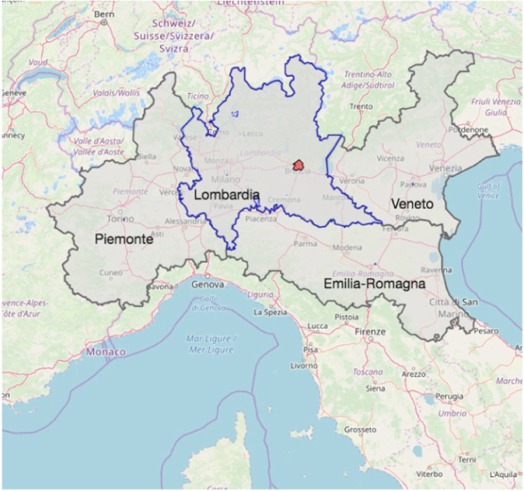
Po Valley in Northern Italy is known as one of the most polluted areas in Europe in terms of particulate matter (PM) and nitrogen dioxide (NO) concentration (EEA, 2019). This is due to the peculiar geographical structure of the area and the exceptional meteorological conditions that do not favour the pollutant dispersion. At the same time the four regions of Po Valley (Lombardia, Emilia Romagna, Piemonte and Veneto, see Fig. 1) are densely populated (with about 23.8 millions inhabitants1 representing about 40% of the total Italian population), heavily industrialised and with a strongly developed agricultural sector. Due to these particular conditions, the air quality thresholds set for human protection are frequently exceeded: the European Environment Agency (EEA) estimates for 2016 that 3.3% of the Po Valley population live in areas where standard levels for three different pollutant were not respected (i.e. PM10 daily limit value, ozone target value and NO2 annual limit value) (EEA, 2019). This has a consequent g impact on human health in terms of premature mortality and morbidity, mainly related to respiratory and cardiovascular diseases. For this reason, air pollution represents the single largest environmental risk in Europe today (Lim et al., 2012) and different statistical approaches can be used for measuring the effects of air pollution exposure on health outcomes (see e.g. Bruno et al., 2016, Blangiardo et al., 2016, Cameletti et al., 2019).
Fig. 1.
The Po Valley regions: Piemonte, Lombardia (with blue borders), Veneto and Emilia-Romagna. The city of Brescia is represented by the red area. (For interpretation of the references to colour in this figure legend, the reader is referred to the web version of this article.)
The earliest cases of Corona virus (COVID-19) occurred in Italy on 31st January 2020,2 followed by a rapid spread of the pandemic starting from the end of February which has led to about 120 thousand cases on 03/04/2020.3 Lombardia has represented the main hotspot being the region with the highest number of infected and dead people with about 47.5 thousand total cases on 03/04/2020. 3 In order to control the COVID-19 spread and the resulting pressure on the healthcare system, on March 8th 2020 the Italian Prime Minister decided the lockdown for the entire Lombardia region, extended to all Italy on the following day. The lockdown decree provides for the closure of schools and universities, for the stop of the non-essential work activities and for ban on people gatherings. Stronger restrictions have been introduced later with subsequent decrees of the Italian government (see the link in footnote 2 for a timeline of the measures taken to manage the Corona virus pandemic).
The lockdown has proved to have a positive effect on air quality in Europe and in the Po Valley in particular. From the analysis of air pollutant concentrations from the 3000 monitoring stations across European countries, the EEA found evidence of a large decrease in air pollutant concentrations.4 Two recent reports by the Copernicus Atmosphere Monitoring Service5 and the Sistema nazionale di protezione ambientale,6 based on the analysis of satellite data, ground observations and numerical modelling outputs, confirm a reduction in the surface concentration of NO in the main European cities and all over the Po Valley. All these reports provide a simple descriptive analysis of an unprecedented situation of low air pollution, without however considering the possible effect of meteorology. For this reason, a statistically robust analysis of the decreasing trend in pollutant concentrations is still missing.
The main aim of this short communication is to evaluate the effectiveness of the lockdown measure (in force since March 8th 2020) on the improvement of air quality. As a particular case study the city of Brescia is considered: it is the second most populated city of the region after Milano, located in the eastern side of Lombardia region (see Fig. 1). Air quality has always been an issue for Brescia who registered in 2018 the unpleasant record of the highest number of exceedances: 47 days of PM10 levels over /m (24-hour mean) and 103 days of ozone concentration over /m (daily maximum 8-hour mean).
The PM10 and NO concentrations recorded from January 1st 2020 to March 27th 20207 by the monitoring stations located in the municipality of Brescia are analysed in order to understand if a significant reduction in air pollution occurred thanks to the lockdown intervention. In this regard, an interrupted time series (ITS, or segmented regression) model is employed (Wagner et al., 2002). This kind of modelling approach is widely used for the evaluation of the longitudinal impact of public interventions or important population related actions. For example, Grundy et al. (2009) quantify the effect of the introduction of 20 mph traffic speed zones on road collisions, injuries, and fatalities in London; Bernal et al. (2016) analyse the effect of the late 2000s financial crisis on suicides in Spain; similarly, Lopez Bernal et al. (2013) study the effects of the Italian smoking ban in public places on hospital admissions for acute coronary events. In the considered case study, the change in the level and/or the trend of PM10 and NO concentrations is modelled by including in a linear regression model a dummy variable and an interaction term. Moreover, to adjust for seasonality and autocorrelation in the response variable, meteorological variables are included in the model and an Autoregressive Moving Average (ARMA) structure for the error term is assumed. In the time series literature this kind of model is also known as ARMAX model (Hyndman and Athanasopoulos, 2019). The analysis is implemented using the forecast package of the R software (R Core Team, 2020).
2. Data
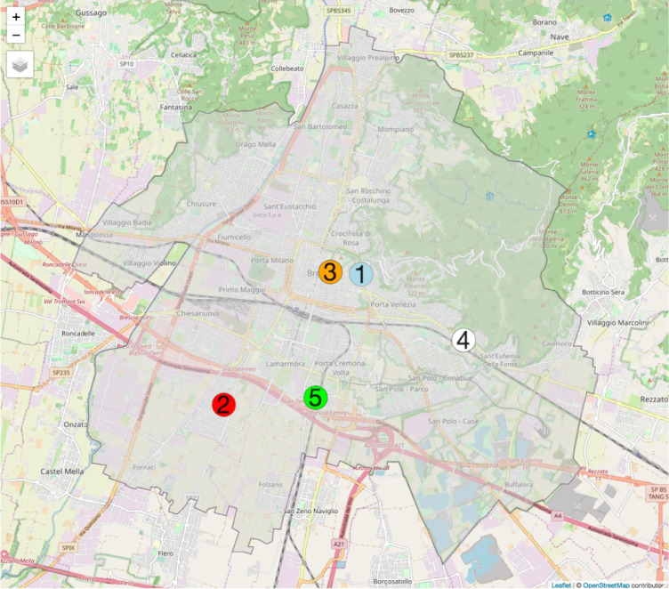
We consider data from January 1st 2020 to March 27th 2020 measured by five air pollutant and weather monitoring stations located in the city of Brescia (see Fig. 2 and Table 1). The data are provided by the Regional Agency for Environmental Protection (ARPA Lombardia). Sensors for measuring concentrations of NO and PM10 are installed in three and two stations, respectively. In particular, station no. 1 and 3 in Fig. 2 are traffic stations located close to the city centre, while station no. 2 is classified as of background type. We include in the analysis meteorological information (temperature, precipitation and wind speed) measured in two stations (number 4 and 5 in Fig. 2). For all the considered variables the daily mean is considered with the exception of precipitation for which the total daily amount is used. Moreover, as the two available temperature time series (from station no. 4 and 5) are strongly and positively correlated (Pearson correlation index = 0.95), the average daily values are computed.
Fig. 2.
Locations of the monitoring stations in Brescia. The numbers in the map refer to column ‘Station ID‘ in Table 1 where the details about the stations and sensors are reported.
Table 1.
Information about monitoring stations and sensors in Brescia for NO and PM10 concentrations and meteorological variables (temperature, precipitation and wind speed).
| Sensor ID | Station ID | Station name | Variable |
|---|---|---|---|
| 6761 | 3 | Broletto | NO (g/m) |
| 6781 | 1 | Via Turati | NO (g/m) |
| 30163 | 2 | Villaggio Sereno | NO (g/m) |
| 6951 | 3 | Broletto | PM10 (g/m) |
| 9961 | 2 | Villaggio Sereno | PM10 (g/m) |
| 2414 | 4 | Pastori | Temperature () |
| 6795 | 5 | Via Ziziola | Temperature () |
| 2417 | 4 | Pastori | Precipitation (mm) |
| 19076 | 4 | Pastori | Wind Speed (m/s) |
3. Methodology
To evaluate if the lockdown in force from March 8th 2020 reduced significantly the PM10 and NO concentrations in the city of Brescia, an interrupted time series regression has been employed for the comparison of the period before (January 1st–March 7th, 2020) and after (March 8th–March 27th, 2020) the containment measure.
Let denote the pollutant concentration (PM10 or NO) at time () measured by a single monitoring station. Moreover, represents the lockdown (L) dummy variable which is equal to 0 for all the time points before the lockdown and 1 afterwards (i.e. from March 8th 2020 to March 27th 2020). The variable represents the time elapsed (in days) starting from January 1st 2020 which is the first considered time point in the analysis ( is the total number of days). The vector contains the values of the considered regressors referred to day given by temperature, precipitation, wind speed and a dummy variable introduced to capture the Sunday effect (the variable is equal to 1 if day occurred on Sunday, and 0 otherwise). The choice of including a variable for Sunday, instead of one for the weekend effect (Saturday–Sunday), is based on a visual inspection of the time series seasonality.
The ITS ARMA model is defined by the two equations: the first includes the intercept, the linear effect of time and of the regressors together with the dummy for the lockdown, which is included also in the interaction term with time. The second equation instead defines the temporal structure of the regression errors. Thus, the model is specified as follows:
| (1) |
| (2) |
In particular, the regression error term follows an ARMA process with coefficients , whereas the innovation error term is assumed to be a Normally distributed white-noise process with zero-mean and variance .
In this model is the vector of coefficients for the regressors. Moreover, represents the baseline level of the response variable when (before the lockdown), whereas is the baseline trend slope, i.e. the expected change in that occurs with each day before the intervention. When the lockdown takes effect, the level and the trend slope become equal to and , respectively. Thus, () represents the post-intervention level (trend slope) change. The final vector of parameters is given by , with , and the maximum likelihood approach is used for estimation (Hyndman and Athanasopoulos, 2019). In particular, a backward stepwise approach is adopted by starting from the full model and by removing the non significant regressors (among temperature, precipitation, wind speed and Sunday dummy variable) according to the value of the -value (the considered threshold is ). The ARMA coefficients are kept in the model even if not significant because they improve the model fit. Also the parameters are not removed from the model in order to discuss the effectiveness of the lockdown intervention in changing the level and trend slope of the time series. The best ARMA structure for the error term is chosen by using the Akaike Information Criterion (AIC) and a residual analysis was carried out in order to assess that the ARMA errors resemble a white-noise series.
4. Results
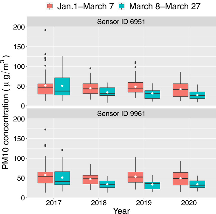
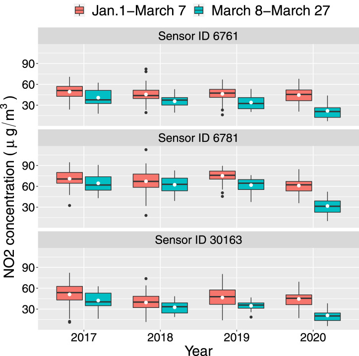
Fig. 3, Fig. 4 display the distribution of PM10 and NO concentrations by sensor and year, separately for the two considered periods: January 1st–March 7th and March 8th–March 27th. It can be observed that for the considered years (2017–2020) the second period is always characterised by lower level of concentrations. This is due to the fact that March is usually the winter month with the most favourable air quality conditions also thanks to the effect of the meteorology. When comparing 2020 with the previous years, no noteworthy differences occur for PM10. Instead, all the NO sensors show for 2020 a more evident difference between the distributions in the two considered time intervals, that could be ascribed to the effect of the lockdown. To assess any significant change in the level and in the trend of the NO and PM10 time series for 2020, five ITS ARMA models are implemented as described in Section 3. All the models include meteorology in order to adjust by the usual decrease in the concentration levels which is expected to be observed in March.
Fig. 3.
Distribution of PM10 concentration by sensor (see Table 1) and year, separately for the two considered periods: January 1st–March 7th and March 8th–March 27th. The white point represents the mean.
Fig. 4.
Distribution of NO2 concentration by sensor (see Table 1) and year, separately for the two considered periods: January 1st–March 7th and March 8th–March 27th. The white point represents the mean.
The parameter estimates for and coefficients are reported in Table 2, Table 3. It can be noted that temperature has no significant effect on concentrations and for this reason it has been omitted from all the models, whereas precipitation has a significant negative effect only for the NO Sensor ID 6781. The most important meteorological variable is wind speed with a negative significant effect for all the models ranging from −13.89 and -5.37. The dummy variable related to the Sunday effect is always significantly different from zero (with a reduction in concentrations) with the exception of the PM10 Sensor ID 6951 located in the city centre of Brescia in a 7 days limited traffic zone.
Table 2.
Estimates of and parameters (and corresponding p-values) for the ITS models implemented for NO time series. If the information is missing it means that the corresponding coefficient was not significantly different from zero and was removed from the model. Besides the covariate coefficients , the following parameters are estimated: the intercept , the baseline trend slope and the post-intervention level (trend slope) change (); see Eq. (1). In particular, and represent the level and the trend slope after the lockdown, to be compared with and , respectively.
| Sensor ID |
||||||
|---|---|---|---|---|---|---|
| 6761 |
6781 |
30163 |
||||
| Est. | -value | Est. | -value | Est. | -value | |
| 62.84 | 0.001 | 78.48 | 0.001 | 61.45 | 0.001 | |
| −0.21 | 0.005 | −0.25 | 0.001 | −0.25 | 0.003 | |
| 54.47 | 0.097 | 94.64 | 0.001 | 43.52 | 0.200 | |
| −0.83 | 0.057 | −1.42 | 0.001 | −0.68 | 0.138 | |
| −0.66 | 0.018 | |||||
| −6.91 | 0.001 | −5.37 | 0.001 | −5.52 | 0.001 | |
| −8.44 | 0.001 | −5.56 | 0.001 | −7.24 | 0.001 | |
Table 3.
Estimates of and parameters (and corresponding p-values) for the ITS models implemented for PM10 time series. If the information is missing it means that the corresponding coefficient was not significantly different from zero and was removed from the model. Besides the covariate coefficients , the following parameters are estimated: the intercept , the baseline trend slope and the post-intervention level (trend slope) change (); see Eq. (1). In particular, and represent the level and the trend slope after the lockdown, to be compared with and , respectively.
| Sensor ID |
||||
|---|---|---|---|---|
| 6951 |
9961 |
|||
| Est. | -value | Est. | -value | |
| 61.48 | 0.001 | 85.72 | 0.001 | |
| −0.25 | 0.0158 | −0.44 | 0.001 | |
| −77.40 | 0.1272 | −41.17 | 0.319 | |
| 0.96 | 0.1458 | 0.65 | 0.218 | |
| −6.97 | 0.0024 | −13.89 | 0.001 | |
| −7.88 | 0.001 | |||
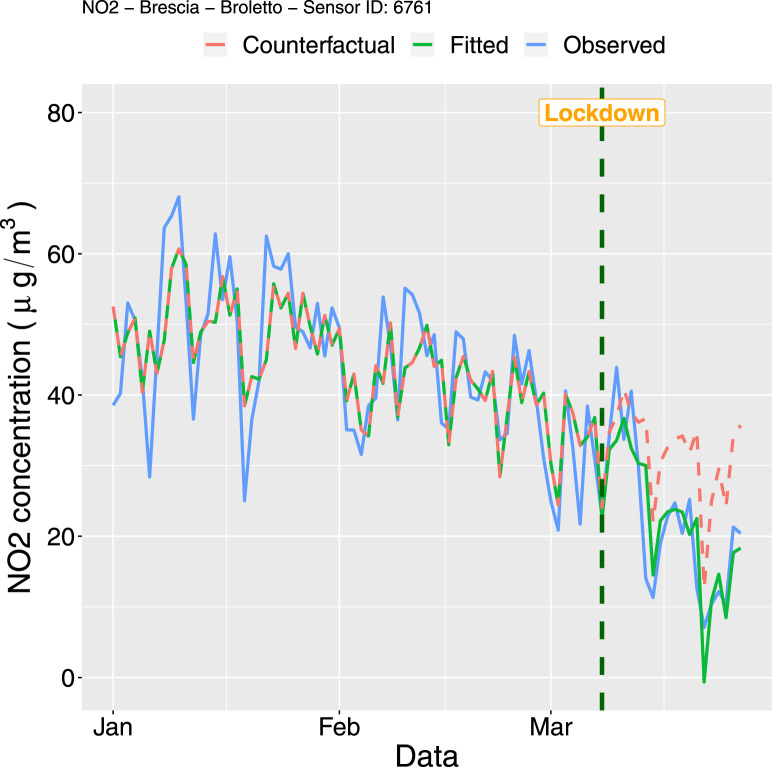
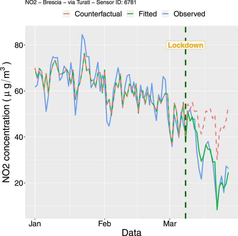
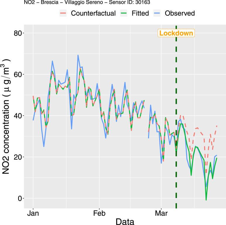
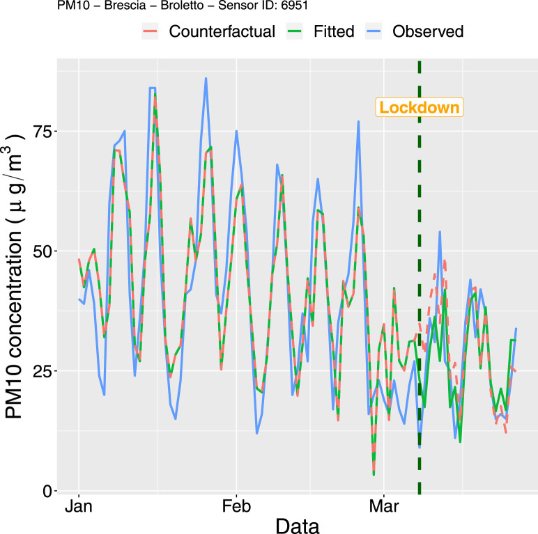
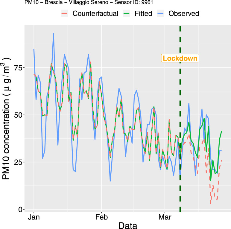
The parameter , which measures the pre-intervention trend slope, is significantly negative for all the five models showing that a somehow decreasing trend was still happening for all the stations (after removing the effect of the other predictors). This is probably related to the spring approaching which favours the pollutant dispersion. The decreasing trend is also evident from the observed time series represented in Fig. 5, Fig. 6, Fig. 7, Fig. 8, Fig. 9 especially for NO concentrations. It is worth to note that a significant change in the level and in the trend after the lockdown occurred only for the NO sensor 6781 (=94.64 and =-1.42, both with -value 0.001). This means that the estimate of the time series slope, i.e. the expected change in the concentration associated with a time unit increase, decreases from −0.25 to −1.67 after the lockdown. This sensor is installed in the station named “Via Turati” which is located next to a heavy-traffic ring road which surrounds the city centre. It is reasonable to suppose that the lockdown intervention has reduced significantly the road traffic along this main artery, which a consequent significant reduction in the NO concentrations. This is coherent with the road transport sector being the most significant contributor of NO emissions (EEA, 2019). For the other two NO stations this effect does not emerge so clearly (although for Sensor ID 6761 the p-values related to and are close to the significance level). This is probability due to the fact that they are located in low traffic areas where the effect of the intervention on traffic reduction was weaker. These results are confirmed by the plots reported in Fig. 5, Fig. 6, Fig. 7, where the observed and fitted (using the estimated parameters reported in Table 2, Table 3) time series are represented together with the counterfactual predictions. The latter represent the expected time series in the hypothetical scenario under which the lockdown had not taken place, i.e. with no intervention and assuming that the time series is stationary after accounting for time-varying confounders. The counterfactual time series is obtained by computing the predicted values of using the parameter estimates obtained from the entire set of data (from January 1st to March 27th, see Table 2, Table 3, Table 4) and assuming that the variable in Eq. (1) is equal to zero for all the time points, whereas the values of the other predictors are kept unchanged. We can observe a more pronounced distance between the observed and counterfactual time series for Sensor ID 6781, whereas for Sensor ID 6761 and 30163 there is no strong evidence of a reduction in NO concentrations following the lockdown. A negligible effect of the intervention is observed also for PM10 concentrations, with the counterfactual series being very close to the observed data as shown in Fig. 8, Fig. 9. Also the parameters and cannot be considered significantly different from zero (see the corresponding estimates reported in Table 3). This could be related to the complexity of the process of PM10 formation, given by the main sources of primary PM (domestic combustion in household heating, road traffic, industrial combustion, agriculture) but also by chemical reactions with other pollutants. It is very likely that the lockdown has reduced the road traffic but at the same time has led to a more intensive use of household heating due to the stay-at-home order.
Fig. 5.
NO2 time series for Sensor ID 6761 from January 1 to March 27 2020: observed time series (blue solid line), fitted values (green solid lines) and counterfactual time series (dashed red line). (For interpretation of the references to colour in this figure legend, the reader is referred to the web version of this article.)
Fig. 6.
NO2 time series for Sensor ID 6781 from January 1 to March 27 2020: observed time series (blue solid line), fitted values (green solid lines) and counterfactual time series (dashed red line). (For interpretation of the references to colour in this figure legend, the reader is referred to the web version of this article.)
Fig. 7.
NO2 time series for Sensor ID 30163 from January 1 to March 27 2020: observed time series (blue solid line), fitted values (green solid lines) and counterfactual time series (dashed red line). (For interpretation of the references to colour in this figure legend, the reader is referred to the web version of this article.)
Fig. 8.
PM10 time series for Sensor ID 6951 from January 1 to March 27 2020: observed time series (blue solid line), fitted values (green solid lines) and counterfactual time series (dashed red line). (For interpretation of the references to colour in this figure legend, the reader is referred to the web version of this article.)
Fig. 9.
PM10 time series for Sensor ID 9961 from January 1 to March 27 2020: observed time series (blue solid line), fitted values (green solid lines) and counterfactual time series (dashed red line). (For interpretation of the references to colour in this figure legend, the reader is referred to the web version of this article.)
In Table 4 the estimates of the ARMA coefficients are reported. Each time series is characterised by its own temporal dynamics: an AR(1) structure is estimated for Sensor ID 6761, MA models of different order arise for Sensor ID 6781, 30163 and 9961, while an ARMA(2,1) is the best choice for Sensor ID 6951. These models give rise to different levels of lag-one autocorrelation: 0.463 for NO Sensor ID 6761, 0.463 for NO Sensor ID 6781, 0.677 for NO Sensor ID 30163, 0.631 for PM10 Sensor ID 6951 and 0.394 for PM10 Sensor ID 9961. The correlation between predicted and observed values is quite high and ranging from 0.823 to 0.939. For all the time series the residuals analysis (results not shown here for the sake of brevity) leads to conclude that the ARMA errors are not significantly different from a Gaussian white-noise.
Table 4.
Specification of the best ARMA model estimated for each NO and PM10 time series and corresponding parameter estimates and p-values (see Eq. (2)).
| Sensor ID 6761 - AR(1) model |
||||
| Est. | 0.463 | |||
| p-value | 0.001 | |||
| Sensor ID 6781 - MA(1) model |
||||
| Est. | 0.673 | |||
| p-value | 0.001 | |||
| Sensor ID 30163 - MA(3) model |
||||
| Est. | 0.737 | 0.656 | 0.230 | |
| p-value | 0.001 | 0.001 | 0.074 | |
| Sensor ID 6951 - ARMA(2,1) model |
||||
| Est. | ||||
| p-value | 0.001 | 0.001 | 0.047 | |
| Sensor ID 9961 - MA(3) model |
||||
| Est. | 0.472 | 0.087 | ||
| p-value | 0.001 | 0.530 | 0.198 | 0.001 |
5. Conclusions
In this paper ITS ARMA models are employed to assess if the lockdown intervention (valid from March 8th 2020) has led to a significant reduction in NO and PM10 concentrations in the city of Brescia. After adjusting by meteorology and weekend effect, the results confirm that a significant change in the level and trend of the time series was observed only for a single NO station located in a heavy traffic zone. The stay-at-home order has certainly lowered road traffic, thus reducing the main emission source connected to NO concentrations. For the remaining NO and PM10 series of data, it is not possible to conclude that the intervention was helpful in improving air quality. This confirms the complexity of air pollution in the Po Valley, where a reduction in emissions does not automatically lead to a significant decrease in concentrations due to the contemporary existence of other important factors (at the local, regional an extra-regional level) such as weather conditions and chemical–physical reactions occurring in the atmosphere. This is particularly relevant if we consider that in the Po Valley, during the winter season, secondary aerosol is the main source for PM (followed by primary emissions from road transport and biomass burning) (Larsen et al., 2012). This explains why the lockdown, which in addition did not have a direct effect on the reduction of the emissions from the agricultural, livestock and residential sector, was not sufficient to reduce significantly and globally the PM concentrations. The same evidence was reported also in Tobías et al. (2020) for the city of Barcelona, in [14] for Salè City (Morocco) and in Li et al. (2020) for the Yangtze River Delta Region (China).
This analysis was conducted only for the city of Brescia. Future work will extend the analysis to all the regions in the Po Valley in order to understand the local differences and point out which are the relevant factors which concur in the dynamics of air pollution in the early months of 2020. In this regard also the methodological approach could be extended to include, for example, a more complex structure for the level, the slope and the seasonality as done in Maranzano et al. (2020) for assessing the impact of a new traffic policy in Milano, Italy. If the entire Po Valley is considered, a spatio-temporal modelling approach, similar to the one proposed in Cameletti et al. (2011), is also an option in order to take also into account the spatial correlation between time series.
CRediT authorship contribution statement
Michela Cameletti: Conceptualization, Methodology, Software, Data curation, Formal analysis, Writing - original draft, Writing - review & editing.
Declaration of Competing Interest
The authors declare that they have no known competing financial interests or personal relationships that could have appeared to influence the work reported in this paper.
Footnotes
Last available data from http://demo.istat.it/ referred to January 1st 2019.
This is the most updated information at the time of writing; for more updated official data from the Italian Ministry of Health, visit http://opendatadpc.maps.arcgis.com/apps/opsdashboard/index.html#/b0c68bce2cce478eaac82fe38d4138b1.
The last days of March are excluded due to an extraordinary event of dust observed on March 28th and 29th which gave rise to an increase in pollutant concentration independent of the lockdown effects.
References
- Bernal J.L., Cummins S., Gasparrini A. Interrupted time series regression for the evaluation of public health interventions: a tutorial. Int. J. Epidemiol. 2016;46(1):348–355. doi: 10.1093/ije/dyw098. [DOI] [PMC free article] [PubMed] [Google Scholar]
- Blangiardo M., Finazzi F., Cameletti M. Two-stage Bayesian model to evaluate the effect of air pollution on chronic respiratory diseases using drug prescriptions. Spatialnd Spatio-Temp. Epidemiol. 2016;18:1–12. doi: 10.1016/j.sste.2016.03.001. [DOI] [PubMed] [Google Scholar]
- Bruno F., Cameletti M., Franco-Villoria M., Greco F., Ignaccolo R., Ippoliti L., Valentini P., Ventrucci M. A survey on ecological regression for health hazard associated with air pollution. Spatial Stat. 2016;18:276–299. [Google Scholar]
- Cameletti M., Gómez-Rubio V., Blangiardo M. Bayesian modelling for spatially misaligned health and air pollution data through the INLA-SPDE approach. Spatial Stat. 2019;31 [Google Scholar]
- Cameletti M., Ignaccolo R., Bande S. Comparing spatio-temporal models for particulate matter in piemonte. Environmetrics. 2011;22(8):985–996. [Google Scholar]
- EEA M. European Environmental Agency (EEA); 2019. Air quality in Europe - 2019 Report: Technical Report. URL https://www.eea.europa.eu/publications/air-quality-in-europe-2019. [Google Scholar]
- Grundy C., Steinbach R., Edwards P., Green J., Armstrong B., Wilkinson P. Effect of 20 mph traffic speed zones on road injuries in London, 1986-2006: controlled interrupted time series analysis. BMJ. 2009;339 doi: 10.1136/bmj.b4469. [DOI] [PMC free article] [PubMed] [Google Scholar]
- Hyndman R., Athanasopoulos G. third ed. OTexts; Melbourne, Australia: 2019. Forecasting: Principles and Practice. URL https://otexts.com/fpp3/. (Accessed 30 March 2020) [Google Scholar]
- Larsen B., Gilardoni S., Stenström K., Niedzialek J., Jimenez J., Belis C. Sources for PM air pollution in the Po Plain, Italy: II. Probabilistic uncertainty characterization and sensitivity analysis of secondary and primary sources. Atmos. Environ. 2012;50:203–213. [Google Scholar]
- Li L., Li Q., Huang L., Wang Q., Zhu A., Xu J., Liu Z., Li H., Shi L., Li R., Azari M., Wang Y., Zhang X., Liu Z., Zhu Y., Zhang K., Xue S., Ooi M.C.G., Zhang D., Chan A. Air quality changes during the COVID-19 lockdown over the yangtze river delta region: An insight into the impact of human activity pattern changes on air pollution variation. Sci. Total Environ. 2020;732 doi: 10.1016/j.scitotenv.2020.139282. [DOI] [PMC free article] [PubMed] [Google Scholar]
- Lim S.S., Vos T., et al. A comparative risk assessment of burden of disease and injury attributable to 67 risk factors and risk factor clusters in 21 regions, 1990-2010: a systematic analysis for the global burden of disease study 2010. Lancet. 2012;380(9859):2224–2260. doi: 10.1016/S0140-6736(12)61766-8. [DOI] [PMC free article] [PubMed] [Google Scholar]
- Lopez Bernal J.A., Gasparrini A., Artundo C.M., McKee M. The effect of the late 2000s financial crisis on suicides in Spain: an interrupted time-series analysis. Eur. J. Publ. Health. 2013;23(5):732–736. doi: 10.1093/eurpub/ckt083. [DOI] [PubMed] [Google Scholar]
- Maranzano P., Fassò A., Pelagatti M., Mudelsee M. Statistical modeling of the early-stage impact of a new traffic policy in Milan, Italy. Int. J. Environ. Res. Publ. Health. 2020;17:1088. doi: 10.3390/ijerph17031088. [DOI] [PMC free article] [PubMed] [Google Scholar]
- Otmani A., Benchrif A., Tahri M., Bounakhla M., Chakir E.M., El Bouch M., Krombi M. Impact of Covid-19 lockdown on PM10, SO2 and NO2 concentrations in Salè City (Morocco) Sci. Total Environ. 2020;735 doi: 10.1016/j.scitotenv.2020.139541. [DOI] [PMC free article] [PubMed] [Google Scholar]
- R Core Team A. R Foundation for Statistical Computing; Vienna, Austria: 2020. R: A Language and Environment for Statistical Computing. URL https://www.R-project.org/ [Google Scholar]
- Tobías A., Carnerero C., Reche C., Massagué J., Via M., Minguillón M.C., Alastuey A., Querol X. Changes in air quality during the lockdown in Barcelona (Spain) one month into the SARS-CoV-2 epidemic. Sci. Total Environ. 2020;726 doi: 10.1016/j.scitotenv.2020.138540. [DOI] [PMC free article] [PubMed] [Google Scholar]
- Wagner A.K., Soumerai S.B., Zhang F., Ross-Degnan D. Segmented regression analysis of interrupted time series studies in medication use research. J. Clin. Pharmacy Therapeut. 2002;27 4:299–309. doi: 10.1046/j.1365-2710.2002.00430.x. [DOI] [PubMed] [Google Scholar]


