A joint model for recurrent events and a semi-competing risk in the presence of multi-level clustering

Abstract

Clinical trial designs often include multiple levels of clustering in which patients are nested within clinical sites and recurrent outcomes are nested within patients who may also experience a semi-competing risk. Traditional survival methods that analyze these processes separately may lead to erroneous inferences as they ignore possible dependencies. To account for the association between recurrent events and a semi-competing risk in the presence of two levels of clustering, we developed a semiparametric joint model. The Gaussian quadrature with a piecewise constant baseline hazard was used to estimate the unspecified baseline hazards and the likelihood. Simulations showed that the proposed joint model has good statistical properties (i.e., <5% bias and 95% coverage) compared to the shared frailty and joint frailty models when informative censoring and multiple levels of clustering were present. The proposed method was applied to data from an AIDS clinical trial to investigate the impact of antiretroviral treatment on recurrent AIDS-defining events (ADE) in the presence of a semi-competing risk of death and multi-level clustering and showed a significant dependency between ADE and death at the patient-level but not at the clinic-level.

1. Background

As the complexity of clinical trial study designs increases, new analytic techniques are needed to adequately address challenging analytical issues. In multi-center clinical trials, for example, participants can be nested within physicians, clinics or healthcare systems, which can lead to a clustering effect. This effect occurs either naturally or by study design because the subjects within a cluster are more correlated than those in other clusters¹. Additionally, participants may experience more than one time-to-event outcome during study follow-up (e.g., recurrent AIDS-defining event (ADE), hospitalization, or injury). These recurrent events nested within a participant create another level of clustering. Often, the repeated impact of these events can negatively affect an individual’s health and potentially result in death^2–4. A death may be associated with the recurrent event process and precludes the event of interest from being observed but not vice versa. Thus, a terminal event, such as death, is referred to as a semi-competing risk^{3, 5}. Figure 1 presents an example of this complex data structure.

Figure 1.

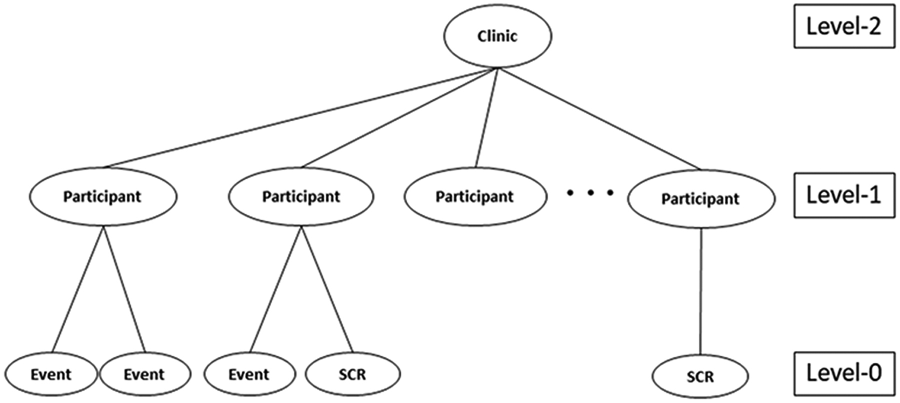
An example of the data structure for the proposed joint model; SCR=Semi-competing risk

Traditional survival methods, such as the Kaplan-Meier estimator or Cox proportional hazards model, are not appropriate for analysis of data with this structure and may lead to erroneous inferences^{6, 7} because no multi-level clustering is considered and they assume death as independent censoring.

Three main analytical approaches have been proposed to address clustering because of recurrent events: variance-corrected models; generalized estimating equations (GEE); and frailty models^7–11. Variance-corrected models treat the correlation between events as a nuisance parameter and account for it by using a robust variance estimator. The model proposed by Andersen et al. extends the proportional hazards model and provides robust standard errors^{8, 11}. Similarly, the Poisson GEE adopts a robust estimator but only focuses on the number of events (count data), so the actual event time is not considered¹⁰. In contrast, frailty models use either gamma or normally distributed random effects (i.e., frailty) in the proportional hazards model to account for the correlation between recurrent events and the unobserved heterogeneity that cannot be explained by observed covariates⁷. Both the GEE and frailty approaches assume a potential correlation between recurrent events within a participant and consider the participants as heterogeneous⁷.

Recently, recurrent events models have been extended to account for either (1) the participant-level association with a semi-competing risk or (2) the multi-level clustering effects with a nested design. For example, Lancaster et al. developed a joint model of recurrent hospitalizations and death by connecting a Poisson process to a time-to-death model through a latent variable to capture the participant-level association¹²; Huang et al. proposed a frailty model for clustered time-to-event data with informative censoring and assumed that participants nested in the same cluster shared a common unmeasured factor affecting the time-to-event and informative censoring¹³; Liu et al. extended the Huang et al. model to a recurrent event process setting to accommodate time-dependent covariates^{13, 14}. In contrast, Sastry¹⁵ and Rondeau et al.¹⁶ developed a nested frailty model in which a higher-level cluster was added to describe the effect of multi-level clustering. For example, Sastry analyzed survival data from a study of children who were nested at both the family and community levels, i.e., clustering at two hierarchical levels¹⁵. Models that ignore community-level clustering effects tend to overestimate the variance of the family-level cluster. Therefore, the variance of the family-level cluster is biased upwards because it includes both unobserved factors from families and communities¹⁵, illustrating the importance of accounting for the effect of different levels of clustering in the nested models to avoid misinterpretation of the frailty variance. Although these models can account for either multiple levels of clustering or for the association between recurrent events (e.g. participant level clustering) and a semi-competing risk, the effect of additional clustering that may occur in a higher-level structure (i.e., clinical sites) has not been incorporated into a recurrent events model with a semi-competing risk^{14, 17}.

Thus, to address this gap, we propose an analytic approach using a joint semiparametric model that incorporates recurrent events, a semi-competing risk, and two levels of clustering (Figure 1). Instead of assuming homogeneity across Level-2 clusters (e.g. clinics), the proposed joint model estimates the variability of both Level-2 and Level-1 clusters (e.g., participants) along with the association between the two survival processes. Thus, to capture the heterogeneity and dependency introduced by hierarchical clustering, the hazards of the recurrent event and semi-competing risk processes will be evaluated at both the participant level and clinical sites level, assuming the hazards can differ by either participants, clinical sites, or both.

Motivating Example:

The OPTions In Management of Antiretrovirals (OPTIMA) trial¹⁸ was designed as a 2×2 factorial clinical trial to compare two treatment strategy options (a) re-treatment with either standard (≤ 4 antiretroviral drugs) or intensive antiretroviral treatment (ART) (>5 antiretroviral drugs) and (b) either treatment starting immediately or following an intended 12-week, monitored ART interruption. Between 2001 and 2006, OPTIMA enrolled 368 patients with advanced multi-drug resistant HIV infection from over 70 clinical centers in the three participating countries (U.S., Canada, and U.K) and followed these patients until the end of study in 2007^{19, 20}. A composite outcome of time-to-first ADE or death from any cause was used as the primary endpoint and analyzed using a Cox model. No significant advantage or disadvantage to any of the two treatment strategies was observed during follow-up; however, it was noted that the confidence limits may include a clinically significant effect that was not reflected in the simple outcome rates¹⁸.

During the course of the study, individuals could experience more than one ADE and subsequently die. The primary analysis did not take the recurrent events nor the semi-competing risk into account. Furthermore, among the 288 Veterans enrolled at 28 Veteran Affairs medical centers (VAMCs), there was strong evidence of heterogeneity in HIV risk. This suggested that heterogeneity should also be investigated at the medical center level in the OPTIMA VA cohort. During a median follow-up of 4 years, 35–37% of Veterans died in each of the four treatment strategy groups and 36% experienced at least one ADE; 23% had only one ADE, while 13% had recurrent ADEs¹⁸. A higher death rate was observed as the number of ADEs per patient increased, regardless of treatment. Veterans with recurrent ADE had a more than 1.4-fold risk of dying compared to those with one ADE, and those with one ADE had nearly twice the risk of dying compared to those with no ADE (data not shown). Thus, there is evidence for a strong association between ADE and death. However, in order to be able to assess this association and heterogeneity at both the participant and VAMC levels, we propose a joint model that connects two semi-parametric frailty models with nested frailties.

In the following article, we describe the proposed joint model, which simultaneously models a recurrent event and semi-competing risk process, while accounting for two levels of clustering. We present results from simulation studies, in which we compare our model with frailty models that ignore multi-level clustering (i.e. joint frailty model) or ignore multi-level clustering and a semi-competing risk process (i.e. shared frailty model). We then apply the proposed model to the VA subgroup of patients in the OPTIMA clinical trial and investigate the impact of ART on recurrent AIDS-defining events (ADE) in the presence of a semi-competing risk of death and multi-level clustering (individual and VAMC). We conclude with a discussion and suggestions for future research.

Methods

The proposed joint model

The proposed model joins two semi-parametric frailty models based on the proportional hazards framework, one for recurrent events and the other for a semi-competing risk process, through two levels of clustering. We let T_ijk = min (X_ijk, C_ij, D_ij) represent the follow-up time for the k^th (k = 1, …,m_ij) event of the j^th (j = 1, …,n_i) participant within clinic i (i = 1, … n), in which the corresponding recurrent event times, independent right censoring times (not by semi-competing risk), and terminal event time (by semi-competing risk) are denoted as X_ijk, C_ij and D_ij, respectively. The last follow-up time is denoted as $T_{ij}^{*}=\text{min}\left(C_{ij},D_{ij}\right)$. The recurrent event indicator, δ_ijk = I (X_ijk = T_ijk), equals 1 if a k^th event is observed from participant j within clinic i, 0 otherwise. The semi-competing risk indicator, ${\mathrm{\Delta }}_{ij}=I\left(T_{ij}^{*}=D_{ij}\right)$, equals 1 if a semi-competing risk is observed, and 0 otherwise. Level-1 covariates (e.g., treatment group) for fixed effects are defined by Z_ijk and Z_ij for the recurrent event and semi-competing risk processes, respectively. Similarly, Level-2 covariates (e.g., treatment assignment in a cluster randomized trial) can be specified to measure the covariate effects on the recurrent event (Z_ij) and semi-competing risk processes (Z_i) at Level-2.

Given two nested frailties, v_i, (Level-2) and w_ij (Level-1), we are able to formulate the following proposed joint model (PJM)

$$r_{ijk}\left(\text{t|}{v}_i,w_{ij}\right)=r_0\left(t\right)\text{exp}\left(\beta Z_{ijk}+v_i+w_{ij}\right)$$ (1)

$${\lambda }_{ij}\left(\text{t|}{v}_i,w_{ij}\right)={\lambda }_0\left(t\right)\text{exp}\left(\alpha Z_{ij}+{\gamma }_2{v}_i+{\gamma }_1{w}_{ij}\right)$$ (2)

where r₀(t) and λ₀(t) indicate the baseline hazard functions of the recurrent event model (equation 1) and semi-competing risk model (equation 2), respectively. We assume the two random effects follow a normal distribution with mean 0 and variance ${\theta }_2^2$ and ${\theta }_1^2$ for Level-2 and Level-1, respectively. In this case, frailties are defined as exp(v_i) and exp(w_ij) and have lognormal distributions [10]. We used normal frailties instead of gamma frailties because there are few existing biological reasons to justify using the gamma distribution over the normal distribution, except for its mathematical convenience^{21, 22}. Furthermore, the flexibility of the normal distribution accommodates complex correlation structures among the observations^{21, 23, 24}.

The parameters β and α represent the effects of covariates (e.g., treatment), which are interpretable as the instantaneous probability of the occurrence of recurrent events and semi-competing risk conditional on the participant’s event history^{14, 17}. The vector of association parameters, γ = (γ₂, γ₁) in equation 2 links the recurrent events and semi-competing risk processes, the larger the value the greater the degree of dependence at Level-2 and Level-1, respectively.

The two different survival processes are independent at either or both levels when the association parameters are zero. The frailties have the same effect on the recurrent events and semi-competing risk processes when γ = 1. When γ is positive or negative, the two processes are positively or negatively correlated, respectively. Note, γ only has interpretation in the presence of significant heterogeneity or when θ = (θ₂, θ₁) is different from zero.

Estimation

The full-likelihood of the PJM given below in equation 3 is the product of components of the recurrent events function (equation 1), semi-competing risk function (equation 2), and the frailty density functions denoted by f(v_i) and f(w_ij).

$$\begin{gathered} L=\prod _{i=1}^n\int \prod _{j=1}^{n_i}\left(\int \mathit{\text{exp}}\left(l_{ijk}^R\cdot l_{ij}^D\right)\cdot f\left(w_{ij}\right)d{w}_{ij}\right)\cdot f\left(v_i\right)d{v}_i \\ =\prod _{i=1}^n\int \prod _{j=1}^{n_i}\left(\prod _{k=1}^{m_{ij}}{\left[r_0\times \left(t_{ijk}\right)\mathit{\text{exp}}\left(\beta Z_{ijk}+v_i+w_{ij}\right)\right]}^{{\delta }_{ijk}}\times \mathit{\text{exp}}\left[-{\int }_0^{t_{ij}^{*}}\mathit{\text{exp}}\left(\beta Z_{ijk}+v_i+w_{ij}\right)\times r_0\left(t_{ijk}\right)dt\right]\times {\left[{\lambda }_0\left(t_{ij}^{*}\right)\text{exp}\left(\alpha Z_{ij}+{\gamma }_2{v}_i+{\gamma }_1{w}_{ij}\right)\right]}^{{\mathrm{\Delta }}_{ij}}\times \mathit{\text{exp}}\left[-{\int }_0^{t_{ij}^{*}}\mathit{\text{exp}}\left(\alpha Z_{ij}+{\gamma }_2{v}_i+{\gamma }_1{w}_{ij}\right)\times {\lambda }_0\left(t_{ij}^{*}\right)\right]\times f\left(w_{ij}\right)d{w}_{ij}\right)\times f\left(v_i\right)d{v}_i \end{gathered}$$ (3)

The unspecified baseline hazard functions for each process are approximated using a piecewise constant function that connects locally constant regions^{25, 26}. Therefore, the hazard is allowed to vary over time but is partially constant over any specified time interval. The piecewise constant model is flexible and gives reasonable results when the time units are small or the true hazard does not dramatically change⁷.

To construct the piecewise constant model, we divided the recurrent events and semi-competing risk times into 5 intervals by every 20^th percentile for the observed number of event times (e.g., $Q_1^R,Q_2^R,\cdots Q_5^R$ and with $Q_0^R=0$ as the smallest recurrent event time). Thus, the piecewise constant baseline hazard of recurrent events is then estimated as $\widetilde{r_0}\left(t\right)={\sum }_{k=1}^5{r}_{0k}I(Q_{k-1}^R<t\le Q_k^R)$ where I(·) denotes an indicator function. The estimated cumulative baseline hazard for recurrent events is derived as $\widetilde{R_0}\left(t\right)={\sum }_{k=1}^5{r}_{0k}max\left(0,\text{min}\left(Q_k^R-Q_{k-1}^R,t-Q_{k-1}^R\right)\right)$. Similarly, the piecewise constant baseline hazard of semi-competing risk time is estimated as $\widetilde{{\lambda }_0}\left(t\right)={\sum }_{k=1}^5{\lambda }_{0k}I\left(Q_{k-1}^D<t\le Q_k^D\right)$ and the estimated cumulative baseline hazard for the semi-competing risk is then derived as $\widetilde{{\mathrm{\Lambda }}_0}\left(t\right)={\sum }_{k=1}^5{\lambda }_{0k}max(0,\text{min}\left(Q_k^D-Q_{k-1}^D,t-Q_{k-1}^D)\right)$. Based on the estimated piecewise constant baseline hazard for each process, the likelihood (equation 3) can be then approximated by replacing the integrals with the estimated baseline hazards. Letting the number of Level-2 and Level-1 clusters be denoted as i = 1, …,n and j = 1, …,n_i, respectively, the estimated log likelihood can be expressed as

$$\widehat{l_{ijk}^R}\cdot \widehat{l_{ij}^D}={\delta }_{ijk}\left[\beta Z_{ijk}+v_i+w_{ij}+\mathit{\text{log}}\widetilde{r_0}\left(t_{ijk}\right)\right]-\mathit{\text{exp}}\left(\beta Z_{ijk}+v_i+w_{ij}\right)\widetilde{R_0}\left(t_{ijk}\right)$$

$$\begin{gathered} +{\mathrm{\Delta }}_{ij}\left[\alpha Z_{ij}+{\gamma }_2{v}_i+{\gamma }_1{w}_{ij}+\mathit{\text{log}}\widetilde{{\lambda }_0}\left(t_{ij}^{*}\right)\right] \\ -\mathit{\text{exp}}\left(\alpha Z_{ij}+{\gamma }_2{v}_i+{\gamma }_1{w}_{ij}\right)\widetilde{{\mathrm{\Lambda }}_0}\left(t_{ij}^{*}\right) \end{gathered}$$

The PJM adopts the Gaussian quadrature (GQ) estimation, which approximates the integral of a parametric function by a weighted average over predetermined abscissas for the frailties^{23, 27}. This method is frequently used for numerical integration in nonlinear mixed effect models^{27, 28}. Lesaffre et al. applied the Gauss-Hermite quadrature rule to calculate the integral of a logistic random effect model²⁸. Ge et al. then applied this rule in the GQ method to approximate the marginal likelihood of the joint likelihood function²⁷. Later, Liu et al. introduced this estimation method into various frailty models to estimate joint likelihood functions²³. This numerical integration method is used because no explicit closed form of the likelihood function exists²³. The GQ method compares favorably with the traditional Expectation-Maximization (EM) algorithm or the modified EM algorithm (e.g., Monte Carlo EM) because it produces accurate estimates while reducing computational burden²³. In addition, both normal and non-normal parametric frailties can be incorporated easily during the estimation²³. The GQ method is implemented by the NLMIXED procedure in SAS 9.4 (SAS Institute Inc.). The annotated code for analysis is described in the appendix. Recently, SAS v. 9.4, SAS Institute, Inc. (TS1M3) has enabled users to include multi-level random statements within the NLMIXED procedure.

Simulations

Simulation studies were conducted to evaluate the performance of the PJM and to compare it with frailty models that ignore multi-level clustering (i.e. joint frailty model) or ignore multi-level clustering and a semi-competing risk process (i.e. shared frailty model). Performance was evaluated for three sample size combinations for Level-1 (e.g., participants) and Level-2 (e.g., clinics): 1) 10 clinics with 30 patients enrolled per clinic; 2) 30 clinics with 10 patients enrolled per clinic; and 3) 20 clinics with 50 enrolled per clinic. Thus, overall samples contained either 300 or 1,000 patients, with an arbitrary average of 1.75 events per participant, similar to the number in OPTIMA. In each setting, we generated two normally distributed nested frailties with mean zero and variances $\left({\theta }_1^2,{\theta }_2^2\right)$ ranging from 1.0 to 4.0. Once the frailties were defined, a binary covariate for treatment group Z_1ij was generated from a binomial distribution with a probability of 0.5. The recurrent events and semi-competing risk processes shared a common Z_1ij, and the coefficients for each covariate were set at β = −0.5 and α = −0.5, respectively. Exponentiation of these coefficients is interpreted as hazard ratios.

An independent censoring time C_ij was generated for each Level-1 cluster (e.g., participants) from a uniform distribution ranging between 0 and 1 resulting in approximately 40% of Level-1 clusters being censored. Conditional on the explanatory variable (Z_1ij) and two frailties w_ij and v_i, the semi-competing risk time D_ij was generated using the hazard function with a baseline hazard λ₀(t) = 2.0. We varied the levels of association at Level-2 (γ₂) from 0.5 to 2.0 (i.e., 0.5, 1.0, 2.0) and maintained a constant Level-1 association (γ₁ = 0.5). If D_ij ≤ C_ij, the semi-competing risk time became the last follow-up time and the semi-competing risk indicator Δ_ij = I(D_ij ≤ C_ij) was set to 1, creating informative censoring; otherwise, the last follow-up was the independent censoring time $T_{ij}^{*}=C_{ij}$ and the semi-competing risk indicator Δ_ij = I(D_ij > C_ij) was set to 0. Next, a recurrent event gap time X_ijk was generated by using the hazard function with a baseline hazard r₀(t) = 1.0. We used the inversion method to transform the recurrent event model followed by a recursive algorithm to generate recurrent survival times^{25, 29, 30}. The observed time of recurrent events $T_{ijk}=\text{min}(D_{ij},C_{ij},{\sum }_{k=1}^j{X}_{ijk})$ was the minimum between the semi-competing risk time, independent censoring time, and cumulative recurrent event time, which is represented in calendar scale time³⁰. This time scale provides information related to disease progression over time since diagnosis, and it is useful when events (or risk) can occur over a long period of time, such as a stroke³⁰. A recurrent time was observed when $T_{ijk}<T_{ij}^{*}$ and δ_ij = I(T_ij = X_ij) = 1; subsequent events were generated while $T_{ijk}<T_{ij}^{*}$ and stopped at $T_{ij}^{*}$ if $T_{ijk}>T_{ij}^{*}$ (δ_ij = 0).

The performance of the frailty models was examined by calculating percent relative bias (i.e., $\left| \frac{\mathit{\text{observed}}-\mathit{\text{true}}}{\mathit{\text{true}}}\right|\times 100$), sampling standard error of the parameter estimate (SE), sampling mean of the standard error estimate (SEM), and coverage probability (CP) of the corresponding 95% confidence interval. Results are based on 300 simulations and are presented for case 1 (10 clinics with 30 enrolled per clinic) below. Results were similar for the other two cases (data not shown).

Effect of Ignoring Level-2 Clustering

The PJM was compared to both the joint frailty model with Level-1 clustering only (JFM-L1) and the shared frailty model with Level-1 clustering only (SFM-L1) to assess the impact of ignoring Level-2 clustering. When holding the association of Level-1 γ₁ constant at 0.5 and varying the degree of association at Level-2 γ₂, the estimates of most parameters of the PJM showed little bias and were efficient (i.e., smaller variance) with CP close to the nominal 0.95 level (Table 1). The treatment effect estimates for the recurrent event process $\left(\widehat{\beta }\right)$ and semi-competing risk process $\left(\widehat{\alpha }\right)$ showed small relative biases ranging from 1.0% to 3.4% and 0.4% to 4.8%, respectively. The CP was also close to the nominal 95% level. The parameters for the association between the two processes at Level-2 $\left(\widehat{{\mathrm{\gamma }}_2}\right)$ and Level-1 $\left(\widehat{{\mathrm{\gamma }}_1}\right)$ were also well-estimated. However, the estimated variance (i.e., standard deviation) of frailty at Level-2 $\left(\widehat{{\theta }_2}\right)$ always showed larger bias and lower CP than at Level-1 $\left(\widehat{{\theta }_1}\right)$. This may result because the total number of Level-2 clusters was smaller than the number of Level-1 clusters. The bias decreased and CP improved when the number of Level-2 clusters increased (data not shown).

Table 1.

Performance of the proposed joint model compared with the joint frailty model and shared frailty models ignoring Level-2 clustering

N=300	Proposed joint model (PJM)					Joint frailty model with Level-1 clustering only (JFM-L1)					Shared frailty model with Level-1 clustering only (SFM-L1)
Parameter	Estimate	Bias	SE	SEM	CP	Estimate	Bias	SE	SEM	CP	Estimate	Bias	SE	SEM	CP
β= −0.5	−0.483	3.4	0.215	0.190	0.944	−0.491	1.8	0.239	0.221	0.947	−0.327	52.9	0.153	0.152	0.787
α= −0.5	−0.502	0.4	0.262	0.284	0.958	−0.521	4.2	0.285	0.287	0.943			NA
γ2= 0.5	0.506	1.2	0.181	0.178	0.986			NA					NA
γ1= 0.5	0.495	1.0	0.236	0.227	0.972	0.514	2.8	0.156	0.151	0.960			NA
θ2 =1.0	0.942	5.8	0.261	0.244	0.901			NA					NA
θ1= 1.0	1.005	0.5	0.105	0.099	0.944	1.356	35.6	0.195	0.110	0.227	0.665	50.4	0.207	0.105	0.234
β= −0.5	−0.487	2.6	0.201	0.190	0.963	−0.501	0.2	0.221	0.221	0.950	−0.346	44.5	0.152	0.159	0.819
α= −0.5	−0.521	4.2	0.296	0.269	0.936	−0.473	5.4	0.297	0.288	0.940			NA
γ2= 1.0	1.060	6.0	0.242	0.207	0.938			NA					NA
γ1= 0.5	0.535	7.0	0.191	0.205	0.951	0.719	43.8	0.172	0.157	0.680			NA
θ2 =1.0	0.929	7.1	0.219	0.239	0.901			NA					NA
θ1= 1.0	0.989	1.1	0.089	0.099	0.988	1.348	34.8	0.187	0.113	0.223	0.673	48.6	0.230	0.117	0.305
β= −0.5	−0.505	1.0	0.209	0.200	0.952	−0.511	2.2	0.229	0.231	0.967	−0.307	62.9	0.167	0.163	0.768
α= −0.5	−0.480	4.0	0.282	0.251	0.912	−0.399	20.2	0.305	0.291	0.917			NA
γ2= 2.0	2.032	1.6	0.367	0.372	0.959			NA					NA
γ1= 0.5	0.534	6.8	0.231	0.218	0.966	0.905	81.0	0.234	0.190	0.413			NA
θ2 =1.0	0.920	8.0	0.256	0.245	0.878			NA					NA
θ1= 1.0	0.985	1.5	0.114	0.110	0.932	1.349	34.9	0.194	0.129	0.270	0.556	79.9	0.180	0.146	0.176

NA: Not Applicable; Percent Relative Bias = mean of $\left|\frac{\mathit{\text{observed}}-\mathit{\text{true}}}{\mathit{\text{true}}}\right|\times 100$; SE = Sampling standard error of the parameter estimate; SEM = Sampling mean of the standard error estimate (SEM); CP = Coverage probability of the corresponding 95% confidence interval

The estimated treatment effect in the recurrent event process $\left(\widehat{\beta }\right)$ in JFM-L1 showed a small bias (i.e., < 5%) similar to the PJM. However, bias of the treatment effect in the semi-competing risk process $\left(\widehat{\alpha }\right)$ increased up to 20% as the association at Level-2 became stronger. The bias in the association parameter at Level-1 $\left(\widehat{{\mathrm{\gamma }}_1}\right)$ increased (up to 81%) as association at Level-2 became stronger. The estimated variance of frailty at Level-1 $\left(\widehat{{\theta }_1}\right)$ was always inflated (~35%) with low CP (22 – 27%). The performance of SFM-L1 was always inferior to those of JFM-L1 and PJM, which showed larger bias and lower CP (Figure 2).

Figure 2.

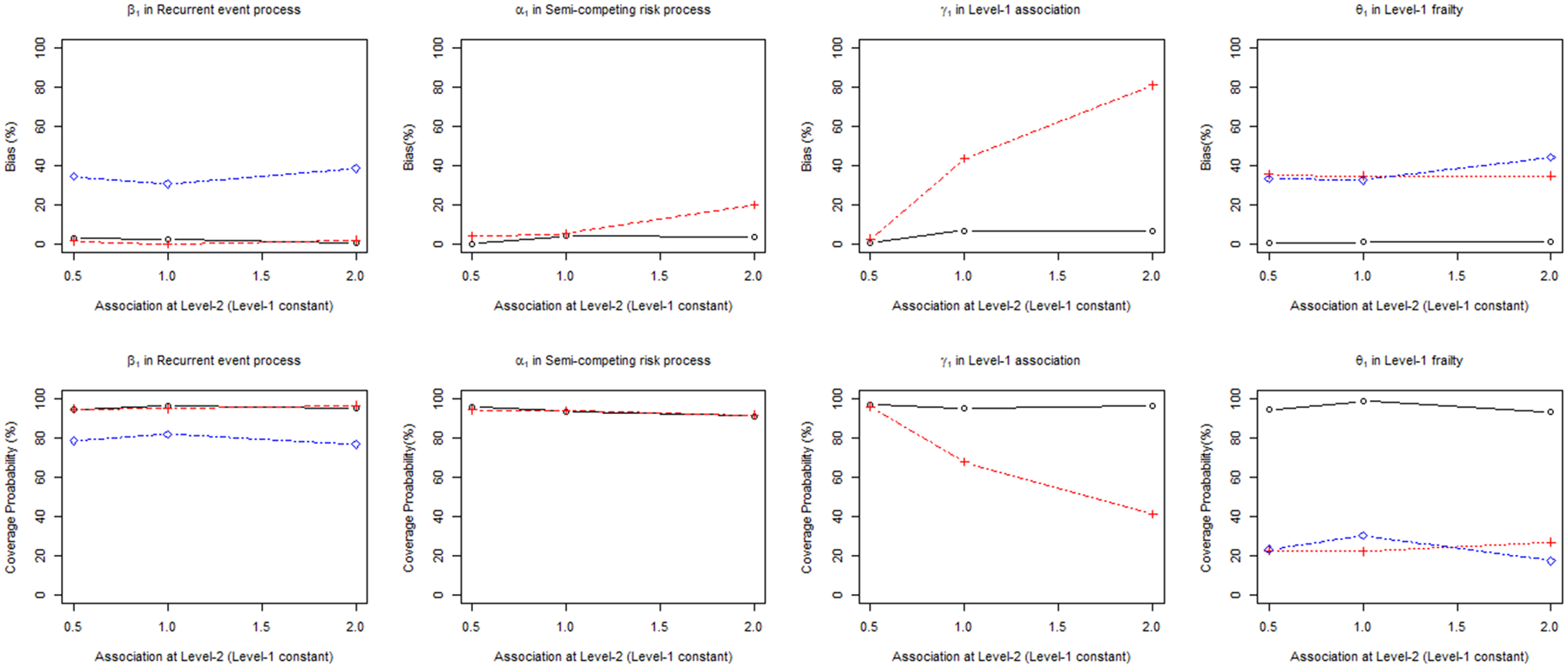
Percent relative bias (%) and coverage probability of β₁, α₁, γ₁, θ₁ in proposed joint model (PJM) versus the joint frailty model (JFM-L1) and shared frailty model (SFM-L1) ignoring Level-2 clustering

Effect of Ignoring Level-1 Clustering

The performance of the PJM was also compared to both the joint frailty model with Level-2 clustering only (JFM-L2) and shared frailty model with Level-2 clustering only (SFM-L2) ignoring clustering at Level-1. Similar to the results above, the parameters of the PJM were relatively unbiased and efficient with a CP close to the nominal level of 0.95 (Table 2). However, in the JFM-L2, the estimated treatment effect in the recurrent event process $\left(\widehat{\beta }\right)$ was inflated compared to the true value (e.g., maximum 13% bias) at all degrees of Level-2 association. While the treatment parameter $\left(\widehat{\beta }\right)$ of the recurrent event process was relatively unbiased in JFM-L1, when the Level-1 clustering is ignored, it became biased. However, the estimated treatment effect in the semi-competing risk process $\left(\widehat{\alpha }\right)$ showed only slightly higher bias than the PJM and it did not increase dramatically with increasing Level-2 association. The bias of the association parameter at Level-2 $\left(\widehat{{\mathrm{\gamma }}_2}\right)$ markedly increased as the association increased. The estimated variance of frailty at Level-2 $\left(\widehat{{\theta }_2}\right)$ for the JFM-L2 was always underestimated; a stronger Level-2 association led to greater underestimation. The performance of the SFM-L2 was generally worse than that of the JFM-L2 and PJM. The estimated treatment effect $\left(\widehat{\beta }\right)$ and variance of frailty in SFM-L2 were highly biased because this model ignores both the Level-1 clustering and semi-competing risk process (Figure 3).

Table 2.

Performance of the proposed joint model compared with the joint frailty model and shared frailty models ignoring Level-1 clustering

N=300	Proposed joint model (PJM)					Joint frailty model with Level-2 clustering only (JFM-L2)					Shared frailty model with Level-2 clustering only (SFM-L2)
Parameter	Estimate	Bias	SE	SEM	CP	Estimate	Bias	SE	SEM	CP	Estimate	Bias	SE	SEM	CP
β= −0.5	−0.483	3.4	0.215	0.190	0.944	−0.453	9.4	0.223	0.103	0.673	−0.268	86.6	0.141	0.105	0.508
α= −0.5	−0.502	0.4	0.262	0.284	0.958	−0.489	2.2	0.273	0.269	0.977			NA
γ2= 0.5	0.506	1.2	0.181	0.178	0.986	0.496		0.167	0.171	0.983			NA
γ1= 0.5	0.495	1.0	0.236	0.227	0.972			NA					NA
θ2 =1.0	0.942	5.8	0.261	0.244	0.901	0.919	8.1	0.238	0.224	0.903	0.547	82.8	0.154	0.152	0.341
θ1= 1.0	1.005	0.5	0.105	0.099	0.944			NA					NA
β= −0.5	−0.487	2.6	0.201	0.190	0.963	−0.435	13.0	0.111	0.059	0.637	−0.299	67.2	0.133	0.112	0.637
α= −0.5	−0.521	4.2	0.296	0.269	0.936	−0.466	6.8	0.157	0.135	0.923			NA
γ2= 1.0	1.060	6.0	0.242	0.207	0.938	1.029	2.9	0.112	0.099	0.930			NA
γ1= 0.5	0.535	7.0	0.191	0.205	0.951			NA					NA
θ2 =1.0	0.929	7.1	0.219	0.239	0.901	0.894	10.6	0.158	0.149	0.833	0.571	75.1	0.174	0.156	0.333
θ1= 1.0	0.989	1.1	0.089	0.099	0.988			NA					NA
β= −0.5	−0.505	1.0	0.209	0.200	0.952	−0.461	7.8	0.216	0.129	0.803	−0.318	57.2	0.164	0.133	0.750
α= −0.5	−0.480	4.0	0.282	0.251	0.912	−0.465	7.0	0.222	0.228	0.990			NA
γ2= 2.0	2.032	1.6	0.367	0.372	0.959	2.368	18.4	0.587	0.431	0.957			NA
γ1= 0.5	0.534	6.8	0.231	0.218	0.966			NA					NA
θ2 =1.0	0.920	8.0	0.256	0.245	0.878	0.796	20.4	0.240	0.203	0.760	0.666	50.2	0.215	0.180	0.557
θ1= 1.0	0.985	1.5	0.114	0.110	0.932			NA					NA

NA: Not Applicable; Percent Relative Bias = mean of $\left|\frac{\mathit{\text{observed}}-\mathit{\text{true}}}{\mathit{\text{true}}}\right|\times 100$; SE = Sampling standard error of the parameter estimate; SEM = Sampling mean of the standard error estimate (SEM); CP = Coverage probability of the corresponding 95% confidence interval

Figure 3.

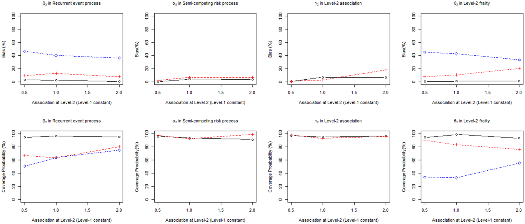
Percent relative Bias and coverage probability of β₁, α₁, γ₁, θ₁ in proposed joint model (PJM) versus joint frailty model (JFM-L2) and shared frailty model (SFM-L2) ignoring Level-1 clustering

Application

We demonstrate the applicability of these methods using our motivating example. We modeled recurrent ADE, the semi-competing risk of death, and considered clustering at the Veteran and VAMC level. The PJM showed no significant effect of either treatment strategy on ADE or death, nor was there an effect of clustering at the VAMC level (Table 3); however, a significant effect of clustering was identified at the Veteran level. The Veteran level random effect parameter was significant for both treatment strategy models (p <0.001 and p <0.001), indicating that more frail Veterans (i.e., estimated random effect > 0) generally had more recurrent events, resulting in a higher risk of death. In contrast, the VAMC-level random effect parameters were not significant for either treatment strategy (p=0.737 and p=0.719). That is, while the unobserved characteristics across VAMCs (e.g., patient management, quality of care) were similar, nested Veterans had significantly different health or other characteristics. Figure 4 plots the estimated frailties for the Level-1 clusters (Veterans) and Level 2 clusters (VAMCs) showing the homogeneity across VAMCs and heterogeneity among Veterans for strategy 1. The findings were similar for strategy 2 (data not shown).

Table 3.

Results of fitting frailty models to the OPTIMA Veterans Cohort

Strategy 1	Shared frailty model		Joint frailty model		Proposed joint model
	HR (95% CI)	p-value	HR (95% CI)	p-value	HR (95% CI)	p-value
Recurrent ADE	1.11 (0.79, 1.56)	0.554	1.08 (0.64, 1.81)	0.771	1.05 (0.64, 1.72)	0.850
Death	NA	NA	1.04 (0.55, 1.95)	0.903	1.06 (0.62, 1.80)	0.830
Veteran-level Cluster	Estimate (SE)	p-value	Estimate (SE)	p-value	Estimate (SE)	p-value
Heterogeneity	0.46 (0.20)	0.024	1.49 (0.16)	<0.001	1.48 (0.16)	<0.001
Association with death	NA	NA	1.17 (0.20)	<0.001	0.97 (0.15)	<0.001
VAMC-level Cluster	Estimate (SE)	p-value	Estimate (SE)	p-value	Estimate (SE)	p-value
Heterogeneity	NA	NA	NA	NA	0.08 (0.23)	0.737
Association with death	NA	NA	NA	NA	0.67 (0.44)	0.878
Strategy 2	Shared frailty model		Joint frailty model		Proposed joint model
	HR (95% CI)	p-value	HR (95% CI)	p-value	HR (95% CI)	p-value
Recurrent ADE	1.01 (0.72, 1.42)	0.936	0.95 (0.57, 1.59)	0.845	0.92 (0.56, 1.51)	0.748
Death	NA	NA	1.20 (0.63, 2.27)	0.586	1.15 (0.68, 1.95)	0.610
Veteran-level Cluster	Estimate (SE)	p-value	Estimate (SE)	p-value	Estimate (SE)	p-value
Heterogeneity	0.46 (0.21)	0.026	1.48 (0.16)	<0.001	1.48 (0.16)	<0.001
Association with death	NA	NA	1.19 (0.21)	<0.001	0.97 (0.15)	<0.001
VAMC-level Cluster	Estimate (SE)	p-value	Estimate (SE)	p-value	Estimate (SE)	p-value
Heterogeneity	NA	NA	NA	NA	0.08 (0.23)	0.719
Association with death	NA	NA	NA	NA	0.67 (0.43)	0.877

NA: Not Applicable; ART = antiretroviral treatment, HR = hazard ratio, CI = confidence interval, ADE = AIDS defining event; Shared frailty model is analyzed without level-2 clustering; joint frailty model is analyzed without level-2 clustering; Strategy 1 = intensive antiretroviral treatment (ART) vs. standard ART; Strategy 2 = ART treatment interruption vs. no interruption

Figure 4.

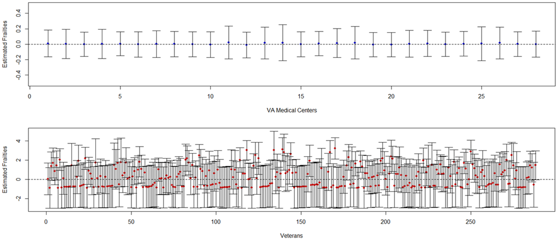
Estimated frailties for Level-2 clusters (VAMC; top panel, blue dots) and Level-1 clusters (Veterans; lower panel, red dots) for Strategy 1: Intensive vs. Standard ART

The association parameter estimates, γ₁, were similar at the Veteran level for both treatment strategies. Both parameter estimates were significant and close to 1, indicating that frailty has approximately the same effect on both ADE and death. However, the VAMC level association parameter estimates, γ₂, were smaller and not significant (p=0.878 and p=0.877 for each treatment strategy). Therefore, it was the frailty of Veterans and not any heterogeneity among VAMCs that contributed to a higher risk for recurrent events and, in turn, a higher risk for death, regardless of treatment strategy.

In comparison, the joint frailty and shared frailty models showed no significant treatment effect on ADE or death regardless of treatment strategy (Table 3), which is also consistent with the primary paper results¹⁸. For both treatment strategies, the joint frailty model revealed significant heterogeneity among patients with respect to recurrent ADE (p < 0.001) and a significant association between recurrent ADE and death (p < 0.001). The heterogeneity and association parameter estimates were similar. In the shared frailty model, the random effect parameters were significant for both treatment strategies (p = 0.024 and p = 0.026); however, the estimates were smaller than those of the joint frailty and PJM models, indicating that the heterogeneity was underestimated.

Discussion

This article addresses a gap in the literature through the proposed joint model (PJM) that incorporates multi-level clustering, a recurrent event process, and a semi-competing risk process. The PJM accounts for the association between the two different survival processes at two different levels of clustering enabling the simultaneous assessment of heterogeneity at both levels. Simulation studies show that the PJM generally yields estimates with low bias and high coverage probability. An advantage of the proposed model over other frailty models is that it can examine the effect of heterogeneity at multiple levels; inference can be highly affected when either level of clustering is ignored. When clustering exists at only one level, a simpler model could be used, such as the joint frailty model or the shared frailty model. Thus, the PJM adds to the armamentarium of methods for analyzing multi-level cluster designs in the presence of a dependent semi-competing risk.

A limitation of the PJM is convergence when the number of Level-2 clusters is small and the semi-competing risk rate is low. The simulation studies showed that the PJM failed to converge when there were ≤7 Level-2 clusters (e.g., clinics) and when the proportion of participants experiencing the semi-competing risk of death was under 10% (e.g., 50 deaths out of 500 subjects) resulting in clusters with a sparse number of events. Practically, the PJM will have convergence problems when applied to studies of recurrent events with a few number of Level-2 clusters and a low number of deaths. Therefore, the PJM will be most applicable to large scale multi-center clinical trials.

The PJM could be extended by incorporating several features that cover analytical issues that are more complex. First, different types of correlated recurrent event processes can be modeled based on the PJM framework. Each recurrent event process can have different degrees of association with a semi-competing risk at different levels. For example, while recurrent ADEs and recurrent serious adverse events (SAEs) may correlate with each other, one process could more strongly be associated with death than the other. In addition, the strength of association can vary across different healthcare systems, states, or countries. Second, the PJM can incorporate a zero-inflated data structure to model subjects who may not experience any primary event of interest. These subjects with no events are presumed to be “unsusceptible” and are termed “structural zeros”^{31, 32}. Furthermore, some clinical sites may have many subjects without any events due to regional or environmental risks suggesting the addition of a zero-inflated structure to the PJM.

Appendix

SAS NLMIXED code for the proposed joint model (PJM)

The user need to verify whether the dataset includes all necessary components (See Supplement Table 1) as the following long format.

Supplement Table 1.

Format of analysis dataset

Clinic	Participant	Time	Event	Treatment
1	1	0.362	1	0
1	1	0.526	1	0
1	1	0.589	0	0
1	2	0.005	2	1
1	3	0.406	1	1
1	3	0.415	2	1
1	4	0.019	2	0
2	1	0.448	1	1
2	1	0.771	2	1

Clinic and Participant represent the Level-2 clusters and Level-1 clusters, respectively. Note that participants are nested within clinics. The Time (i.e., time-to-event) is described in total time scale (i.e., cumulative) and Event is categorized into 3 levels; Event=1 indicates recurrent event, Event=2 indicates semi-competing risk, and Event=0 indicates censoring. Treatment is an independent variable. Note that SAS NLMIXED requires dummy coding when the levels are more than two.

The NLMIXED procedure calculates the piecewise constant baseline hazard for each process and plugs it into the likelihood. Necessary components are described in Supplement Table 2. For detail questions, please contact the first author (ryan.taehyun.jung@gmail.com)

Supplement Table 2.

Corresponding components in the analysis code

Component	Note
r01– r05	Initial values for piecewise constant baseline hazard for recurrent events
h01–h05	Initial values for piecewise constant baseline hazard for semi-competing risk
qr0 – qr100	Quintile for recurrent event times†
qd0 – qd100	Quintile for semi-competing risk times†
dur_r1 – dur_r5	Duration between quintile for recurrent event times
dur_d1 – dur_d5	Duration between quintile for semi-competing risk time
event_r1 – event_r5	Recurrent event indicator in the dur_r1 – dur_r5
event_d1 – event_d5	Semi-competing risk indicator in the dur_d1 – dur_d5
base_haz_r / base_haz_d	Baseline hazard for recurrent events / semi-competing risk
cum_base_haz_r / cum_base_haz_d	Cumulative baseline hazard for recurrent events / semi-competing risk
mu1 / mu2	Linear predictor for recurrent events / semi-competing risk

^†Time is divided into 5 intervals by every 20^th percentile (See 2.2 Estimation)

PROC NLMIXED data=all qpoints=10 maxiter=2000; 
parms r01=0.01 r02=0.01 r03=0.03 r04=0.03 r05=0.05 
h01=0.01 h02=0.03 h03=0.03 h04=0.05 h05=0.05   
beta1 0.10 alpha1 −0.1 gamma2 0.7 gamma1 1.0 theta2 0.6   theta1 1.0; /*Initial values */
bounds r01 r02 r03 r04 r05 h01 h02 h03 theta theta2 >=0;
/* baseline hazard & cum baseline hazard for recurrent events */
base_haz_r= r01*event_r1 + r02*event_r2 + r03*event_r3 + r04* event_r4 + r05*event_r5;
cum_base_haz_r=r01*dur_r1 + r02*dur_r2 + r03*dur_r3 + r04*dur_r4 + r05*dur_r5;
/* baseline hazard & cumulative baseline hazard for a semi-competing risk */
base_haz_d = h01*event_d1 + h02*event_d2 + h03*event_d3 + h04*event_d4 + h05*event_d5;
cum_base_haz_d = h01*dur_d1 + h02*dur_d2 + h03*dur_d3 + h04*dur_d4 + h05*dur_d5;
mu1= beta1 * TRT + v + w; /* for recurrent event process */   
mu2= alpha1 * TRT + gamma2 * v + gamma1 * w; /* for semi-competing risk process */   
loglik1 = -exp(mu1) * cum_base_haz_r;
loglik2 = -exp(mu2) * cum_base_haz_d;
if Event=1 then loglik = log(base_haz_r) + mu1;
if Event=2 then loglik = log(base_haz_d) + mu2 +loglik1+loglik2;
if Event=0 then loglik = loglik1+loglik2;
MODEL Time ~ general(loglik);
RANDOM v ~ normal(0,exp(2*log(theta2))) subject = Sites  out=v_est;  /* For the Level-2 random effect v(i)*/   
RANDOM w ~ normal(0,exp(2*log(theta1))) subject = Patid(Sites)  out=w_est; /* For the Level-1 random effect wj(i)*/   
run;

References

- 1.Fitzmaurice GM. Clustered Data. Encyclopedia of Statistics in Behavioral Science. 2005. [Google Scholar]
- 2.Ghosh D Semi-parametric inferences for association with semi-competing risks data. Stat Med. 2006; 25: 2059–70. [DOI] [PubMed] [Google Scholar]
- 3.Haneuse S and Lee KH. Semi-Competing Risks Data Analysis Accounting for Death as a Competing Risk When the Outcome of Interest Is Nonterminal. Circ-Cardiovasc Qual. 2016; 9: 322–31. [DOI] [PMC free article] [PubMed] [Google Scholar]
- 4.Wang MC, Qin J and Chiang CT. Analyzing Recurrent Event Data With Informative Censoring. J Am Stat Assoc. 2001; 96. [DOI] [PMC free article] [PubMed] [Google Scholar]
- 5.Peng LM, Jiang HY, Chappell RJ and Fine JP. An Overview of the Semi-Competing Risks Problem. Wiley Ser Probab St. 2008: 177–92. [Google Scholar]
- 6.Cai J and Schaubel DE. Analysis of Recurrent Event Data. 2003.
- 7.Wienke A Frailty models in survival analysis. Chapman and Hall/CRC; 1 edition, 2010. [Google Scholar]
- 8.Andersen PK and Gill RD. Cox Regression-Model for Counting-Processes - a Large Sample Study. Ann Stat. 1982; 10: 1100–20. [Google Scholar]
- 9.Guo Z, Gill TM and Allore HG. Modeling repeated time-to-event health conditions with discontinuous risk intervals. An example of a longitudinal study of functional disability among older persons. Methods Inf Med. 2008; 47: 107–16. [PMC free article] [PubMed] [Google Scholar]
- 10.Matsui S Sample size calculations for comparative clinical trials with over-dispersed Poisson process data. Statistics in Medicine. 2005; 24: 1339–56. [DOI] [PubMed] [Google Scholar]
- 11.Prentice RL, Williams BJ and Peterson AV. On the Regression-Analysis of Multivariate Failure Time Data. Biometrika. 1981; 68: 373–9. [Google Scholar]
- 12.Lancaster T and Intrator O. Panel data with survival: Hospitalization of HIV-positive patients. Journal of the American Statistical Association. 1998; 93: 46–53. [Google Scholar]
- 13.Huang X and Wolfe RA. A frailty model for informative censoring. Biometrics. 2002; 58: 510–20. [DOI] [PubMed] [Google Scholar]
- 14.Liu L, Wolfe RA and Huang X. Shared frailty models for recurrent events and a terminal event. Biometrics. 2004; 60: 747–56. [DOI] [PubMed] [Google Scholar]
- 15.Sastry N A nested frailty model for survival data, with an application to the study of child survival in northeast Brazil. J Am Stat Assoc. 1997; 92: 426–35. [DOI] [PubMed] [Google Scholar]
- 16.Rondeau V, Filleul L and Joly P. Nested frailty models using maximum penalized likelihood estimation. Stat Med. 2006; 25: 4036–52. [DOI] [PubMed] [Google Scholar]
- 17.Rondeau V, Mathoulin-Pelissier S, Jacqmin-Gadda H, Brouste V and Soubeyran P. Joint frailty models for recurring events and death using maximum penalized likelihood estimation: application on cancer events. Biostatistics. 2007; 8: 708–21. [DOI] [PubMed] [Google Scholar]
- 18.Holodniy M, Brown ST, Cameron DW, et al. Results of antiretroviral treatment interruption and intensification in advanced multi-drug resistant HIV infection from the OPTIMA trial. PLoS One. 2011; 6: e14764. [DOI] [PMC free article] [PubMed] [Google Scholar]
- 19.Kyriakides TC, Babiker A, Singer J, et al. An open-label randomized clinical trial of novel therapeutic strategies for HIV-infected patients in whom antiretroviral therapy has failed: rationale and design of the OPTIMA Trial. Control Clin Trials. 2003; 24: 481–500. [DOI] [PubMed] [Google Scholar]
- 20.Kyriakides TC, Babiker A, Singer J, Piaseczny M and Russo J. Study conduct, monitoring and data management in a trinational trial: the OPTIMA model. Clin Trials. 2004; 1: 277–81. [DOI] [PubMed] [Google Scholar]
- 21.Belot A, Rondeau V, Remontet L, Giorgi R and group Cws. A joint frailty model to estimate the recurrence process and the disease-specific mortality process without needing the cause of death. Stat Med. 2014; 33: 3147–66. [DOI] [PubMed] [Google Scholar]
- 22.Hirsch K and Wienke A. Software for semiparametric shared gamma and log-normal frailty models: An overview. Comput Meth Prog Bio. 2012; 107: 582–97. [DOI] [PubMed] [Google Scholar]
- 23.Liu L and Huang X. The use of Gaussian quadrature for estimation in frailty proportional hazards models. Stat Med. 2008; 27: 2665–83. [DOI] [PMC free article] [PubMed] [Google Scholar]
- 24.Rondeau V, Schaffner E, Corbiere F, Gonzalez JR and Mathoulin-Pelissier S. Cure frailty models for survival data: Application to recurrences for breast cancer and to hospital readmissions for colorectal cancer. Stat Methods Med Res. 2013; 22: 243–60. [DOI] [PubMed] [Google Scholar]
- 25.Bender R, Augustin T and Blettner M. Generating survival times to simulate Cox proportional hazards models. Stat Med. 2005; 24: 1713–23. [DOI] [PubMed] [Google Scholar]
- 26.Gharibvand L and Liu L. Analysis of survival data with clustered events SAS Global Forum. Citeseer, 2009, p. 1–11. [Google Scholar]
- 27.Ge Z, Bickel PJ and Rice JA. An approximate likelihood approach to nonlinear mixed effects models via spline approximation. Computational Statistics & Data Analysis. 2004; 46: 747–76. [Google Scholar]
- 28.Lesaffre E and Spiessens B. On the effect of the number of quadrature points in a logistic random effects model: an example. J Roy Stat Soc C-App. 2001; 50: 325–35. [Google Scholar]
- 29.Jahn-Eimermacher A, Ingel K, Ozga AK, Preussler S and Binder H. Simulating recurrent event data with hazard functions defined on a total time scale. BMC Med Res Methodol. 2015; 15: 16. [DOI] [PMC free article] [PubMed] [Google Scholar]
- 30.Pénichoux J, Moreau T and Latouche A. Simulating recurrent events that mimic actual data: a review of the literature with emphasis on event-dependence. arXiv preprint arXiv:150305798. 2015. [Google Scholar]
- 31.Wong KY and Lam KF. Modeling zero-inflated count data using a covariate-dependent random effect model. Statistics in Medicine. 2013; 32: 1283–93. [DOI] [PubMed] [Google Scholar]
- 32.Liu L, Huang XL, Yaroshinsky A and Cormier JN. Joint Frailty Models for Zero-Inflated Recurrent Events in the Presence of a Terminal Event. Biometrics. 2016; 72: 204–14. [DOI] [PubMed] [Google Scholar]