

Abstract
Stratospheric intrusions have been the interest of decades of research for their ability to bring stratospheric ozone (O3) into the troposphere with the potential to enhance surface O3 concentrations. However, these intrusions have been misrepresented in models and reanalyses until recently, as the features of a stratospheric intrusion are best identified in horizontal resolutions of 50 km or smaller. NASA’s Modern-Era Retrospective Analysis for Research and Applications Version-2 (MERRA-2) reanalysis is a publicly-available high-resolution dataset (~50 km) with assimilated O3 that characterizes O3 on the same spatiotemporal resolution as the meteorology. We demonstrate the science capabilities of the MERRA-2 reanalysis when applied to the evaluation of stratospheric intrusions that impact surface air quality. This is demonstrated through a case study analysis of stratospheric intrusion-influenced O3 exceedences in spring 2012 in Colorado, using a combination of observations, the MERRA-2 reanalysis and the Goddard Earth Observing System Model, Version 5 (GEOS-5) simulations.
1. Introduction
Surface ozone (O3) is harmful to human health and agriculture [Scherrer et al., 2006; Krzyzanowski and Cohen, 2008]. Near the surface, O3 is termed a secondary pollutant since it is a product of the photochemical reaction with precursors such as nitrogen oxides (NOx; NO and NO2), carbon monoxide (CO) and non-methane hydrocarbons which have both man-made and natural emission sources in the troposphere. Therefore, in order to reduce near surface O3 concentrations, communities must reduce anthropogenic pollution sources. However, the injection of stratospheric O3 into the troposphere, known as a stratospheric intrusion (SI), can also lead to concentrations of ground-level O3 exceeding the national ambient air quality standard (NAAQS) set by the Environmental Protection Agency (EPA), especially at high elevations [e.g., Langford et al., 2009, 2015; Lin et al., 2012, 2014; Yates et al., 2013; Zhang et al., 2014]. In October 2015, the EPA revised the US NAAQS for daily maximum 8-hour average (MDA8) O3 from 75 parts per billion by volume (ppbv) to 70 ppbv [U.S. Environmental Protection Agency, 2015]. Therefore, it is crucial that we are able to understand, model, and predict SIs and their potential impact on surface O3 concentrations.
SIs form as a result of the tropopause being drawn down below the jet stream, referred to as tropopause folding, often associated with an upper-level trough. SIs are characterized by O3-rich [e.g., Danielsen, 1968; Shapiro, 1974, 1980; Holton et al., 1995; Browning, 1997] and CO-poor [Fischer et al., 2000] air, with relatively high levels of potential vorticity (PV) [Holton et al., 1995] and low levels of water vapor often observed in satellite imagery as a “dry slot” [e.g., Bader et al., 1995; Wimmers et al., 2003]. Therefore, tropopause folds can lead to the mixing of stratospheric and tropospheric air with different chemical and meteorological properties at low altitudes [e.g., Danielsen, 1980; Shapiro, 1980; Holton et al., 1995], remaining behind a mid-latitude cyclone’s surface cold front [Browning, 1997; Bethan et al., 1998; Cooper et al., 2001; Knowland et al., 2015]. The west coast of the USA is located at the end of the Pacific Ocean storm track [e.g. Hoskins and Hodges, 2002], a region favorable for stratosphere-to-troposphere transport of O3 [James et al., 2003; Sprenger and Wernli, 2003; Stohl et al., 2003; Škerlak et al., 2014]. On the lee-side of the Rocky Mountains, cyclones form (or redevelop) supported by upper-level troughs [McClain, 1960; Carlson, 1991]. However, the descending motion associated with the upper-level trough can still be a strong feature in the troposphere over the Rocky Mountains, prior to the identification of a surface low pressure system. In the upper-level flow, the troughs can form closed lows and even become “cut-offff” from the westerly flow [Palmén and Newton, 1969]. This can result in the prolonged influence of the tropopause folds on tropospheric O3 concentrations over a region [Lin et al., 2012; Yates et al., 2013] until the cut-offff low (COL) dissipates or is reabsorbed into the mean flow [Nieto et al., 2008]. During the winter and spring, there is a build-up of O3 in the lower stratosphere, and this leads to SIs having the largest influence on surface O3 in the spring [Danielsen and Mohnen, 1977; Holton et al., 1995; Monks, 2000].
For over 40 years, studies have observed the injection of O3-rich air into the troposphere within tropopause folds over western USA [e.g., Lovill, 1970; Shapiro, 1980; Langford et al., 1996, 2009, 2012; Wimmers et al., 2003; Cooper et al., 2004; Lefohn et al., 2011] with recent studies focusing on the impact of SIs on O3 air quality exceedences in the high elevation communities of the Rocky Mountains [e.g., Langford et al., 2009, 2015; Lin et al., 2012, 2014; Yates et al., 2013; Zhang et al., 2014]. Langford et al. [2009] focused on the transport of stratospheric O3 in Colorado’s Front Range during the spring of 1999 using lidar and surface measurements of O3. They identified high concentrations of O3 in the mid-troposphere down to the surface as a result of tropopause folds associated with upper-level troughs in the region. Lin et al. [2012] utilized the abundance of vertical observations from ozonesondes and lidar taken during the 2010 NOAA Cal-Nex field campaign in California as well as ground-based measurements throughout western USA, in conjunction with a model study to quantify the stratospheric fraction of air that impacts NAAQS exceedence events. Using the NOAA Geophysical Research Laboratory (GFDL) Atmosphere Model version 3 (AM3) with fully coupled stratosphere-troposphere chemistry at ~50 km resolution, Lin et al. [2012] attributed 50–60 % of total modelled surface O3 in spring 2010 (as much as 20–40 ppbv of additional O3 during 4 deep intrusions) to stratospheric origins on exceedence days. Using a coarser resolution model (~200 km), Lin et al. [2015] extended the analysis to April and May during a 23-year period (1990–2012) and found the average stratospheric O3 contribution is 15–25 ppbv of western US surface O3.
While the impact of SIs on surface O3 in the western US is well documented, simulating and predicting such events remains challenging. The resolutions of current global meteorological analyses (~10–50 km) are sufficient for resolving the dynamical evolution of SIs, however these models typically contain very limited representations of trace gases like O3. Reanalyses have been used in numerous studies to explore the frequency, spatial variations and structure of SIs [e.g., Stohl and Trickl, 1999; Waugh and Polvani, 2000; Sprenger and Wernli, 2003; Lefohn et al., 2011; Reutter et al., 2015; Nath et al., 2016], however, there are very few such studies which also use reanalysis O3 [Škerlak et al., 2014; Zanis et al., 2014; Knowland et al., 2015, 2017; Ott et al., 2016; Ryoo et al., 2017]. It is our objective to investigate whether NASA’s Modern-Era Retrospective Analysis for Research and Applications Version-2 (MERRA-2) reanalysis, which is similar to NASA’s Global Modeling and Assimilation Office (GMAO) operational forecasting system, is able to capture the dynamical features of a SI, in particular the isentropic descent of elevated O3 within and below the tropopause fold. Such datasets would support air quality agencies for more rapid identification of the impact of stratospheric air on ground-level O3 [Kaldunski et al., 2017] separate from local sources or the long-range transport of O3 [Ryoo et al., 2017]. The focus of this study will be on springtime (March - June (MAMJ)) O3 air quality exceedences in 2012 which were identified by the EPA as having direct connection with SIs [US EPA AQS database, 2017].
2. Data
2.1. Observational datasets
In the spring of 2012, there were seven days when the MDA8 O3 [EPA AirData, 2016] at the Rocky Mountain National Park (RMNP) Long’s Peak monitoring station (40.27°N, 105.54°W, 2742 m, Air Quality System (AQS) Site ID 08-069-0007, located ~100 km northwest of Denver) exceeded the NAAQS of 75 ppbv as a result of SIs [US EPA AQS database, 2017]: March 26th, April 6th, April 27th, May 26–28th, and June 14th. Several other suburban and rural monitoring stations in Colorado also reported exceedences related to SIs on these and other dates in spring 2012 [US EPA AQS database, 2017]. Less than half of the diurnal variation in the hourly MAMJ O3 at RMNP can be explained by the 1st (diurnal) harmonic, therefore other drivers in the O3 variability must be considered. Deep SIs, those which impact surface O3 concentrations, were anomalously frequent in the western USA in the spring of 2012 compared to the 1990–2012 period [Lin et al., 2015], and observed MDA8 O3 was also found to have a maximum in the western USA that spring for the period 2004–2012 [Baylon et al., 2016]. This study will explore the representation of two of the SIs in remote sensing observations and the Goddard Earth Observing System Model, Version 5 (GEOS-5) model and assimilation products. The first case study in early spring (March 26th local time (LT; +07:00 UTC) hereafter will be referred to as the SI-1 event and the second case study, which occurred in late spring (May 26–28th event LT), will be referred to as the SI-2 event.
Daily total column O3 (TCO) and relative humidity (RH) from the Atmospheric Infrared Sounder (AIRS) on NASA’s Aqua satellite are used to identify the presence of SIs over RMNP in observational data and to validate MERRA-2 reanalysis TCO since the AIRS O3 data were not assimilated in MERRA-2. AIRS is equipped to measure both meteorological variables and chemical profiles [Aumann et al., 2003; Susskind et al., 2006; Chahine et al., 2006] and observes the surface twice daily (01:30 and 13:30 LT). The retrievals are performed even when clouds are present which makes the dataset ideal when analyzing regions near mid-latitude cyclones. The AIRS team produces several datasets of different spatiotemporal resolution. We use the level 3 version 6 (L3 V6) at 1° horizontal resolution [AIRS Science Team/Joao Texeira, 2013].
2.2. Model datasets
NASA’s MERRA-2 reanalysis is an ideal candidate to explore the vertical structure of the SIs over RMNP as it is a publicly-available, high-resolution reanalysis dataset (0.5° × 0.625° latitude-by-longitude grid, nominally ~50 km in the latitudinal direction, 72 model layers up to 0.01 hPa [Bosilovich et al., 2016; Gelaro et al., 2017]) which assimilates both O3 and meteorological observations [Bosilovich et al., 2015; McCarty et al., 2016; Gelaro et al., 2017]. The MERRA-2 reanalysis covers the period from January 1, 1980 to within a couple weeks of real time and is the product of the GEOS-5 data assimilation system (DAS) [Bosilovich et al., 2015; Gelaro et al., 2017]. The GEOS-5 model includes monthly-averaged ozone production and loss rates linearly interpolated to daily values for both the stratosphere and the troposphere [Bosilovich et al., 2016]. After 2004, MERRA-2 assimilates satellite retrievals of TCO from the Ozone Monitoring Instrument (OMI; Levelt et al. [2006]) and stratospheric O3 profiles from the Microwave Limb Sounder (MLS; Waters et al. [2006]) [Bosilovich et al., 2015; McCarty et al., 2016; Gelaro et al., 2017]. MERRA-2 O3 in the lower stratosphere is well-represented and has been shown to agree with ozonesondes [Wargan et al., 2015, 2017]; therefore, where there is direct influence of stratospheric O3 into the troposphere, such as an SI, we can expect realistic intrusions although possibly biased since the background ozone in the troposphere is simulated by simple chemistry parametrization [Ott et al., 2016].
The meteorological and chemical variables – winds (u, υ), vertical velocity (ω), equivalent potential temperature (θe; calculated from temperature and specific humidity), Ertel’s PV (EPV), RH and O3 mixing ratios – were extracted on pressure levels up to 150 hPa [GMAO, 2015a]. In addition, MERRA-2 sea-level pressure (SLP) [GMAO, 2015b] and TCO [GMAO, 2015c] are used in the comparison to the AIRS retrievals.
Two additional model variables are used: GEOS-5 simulated CO using emissions described in Ott et al. [2010] and an idealized stratospheric “influence” tracer (STFR) from Ott et al. [2016]. The STFR is set to 1 in the stratosphere and to 0 at the surface. For the STFR simulation, the tropopause was the higher height of the thermal tropopause or the dynamical tropopause. In the GEOS model, the dynamical tropopause is defined as the 3 PVU isosurface, where 1 PV unit (PVU) = 10−6 K m2 kg−1 s−1, which is higher than the conventional 2 PVU isosurface [Holton et al., 1995].
3. Results
The 8-hour running average O3 and the hourly average O3 observed at RMNP and the corresponding 3-hourly surface O3 from MERRA-2 [GMAO, 2015d] are presented here for spring of 2012 (Fig. 1b). During the SI-1 event, the observed hourly O3 at RMNP ≥ 75 ppbv for 7 hours (1 hour March 26th and 6 hours March 27th, based on UTC, Fig. 1a) with the maximum observed hourly O3 equal to 87 ppbv observed at March 27, 2012 00UTC (Fig. 1b; MERRA-2 O3 = 58 ppbv). The second intrusion event, SI-2, influenced ground-level O3 for several days at RMNP; observed hourly O3 ≥ 75 ppbv for 11 hours during this 3-day period (Fig. 1a) with maximum observed hourly O3 of 91 ppbv at 09 UTC on May 27, 2012 (Fig. 1b; MERRA-2 O3 = 65 ppbv). Considering the new NAAQS value for MDA8 O3, RMNP observed hourly O3 ≥ 70 ppbv for 11 hours during the SI-1 event and 30 hours for the SI-2 event (Fig. 1a). Figure 1 highlights the doubling of possible exceedence days if the new MDA8-O3 NAAQS of 70 ≥ ppbv is applied to 2012. As expected, the MERRA-2 surface O3 for the grid box closest to RMNP underestimates the O3 variability of a point source measurement (r2 = 0.34, based on 968 3-hourly timesteps; Fig. 1b) in part because of the simple O3 chemistry in the GEOS-5 model; however, there are spikes in the reanalysis O3 at or near the times of observed O3 exceedences, portraying the influence of stratospheric O3 on the grid-box.
Figure 1.
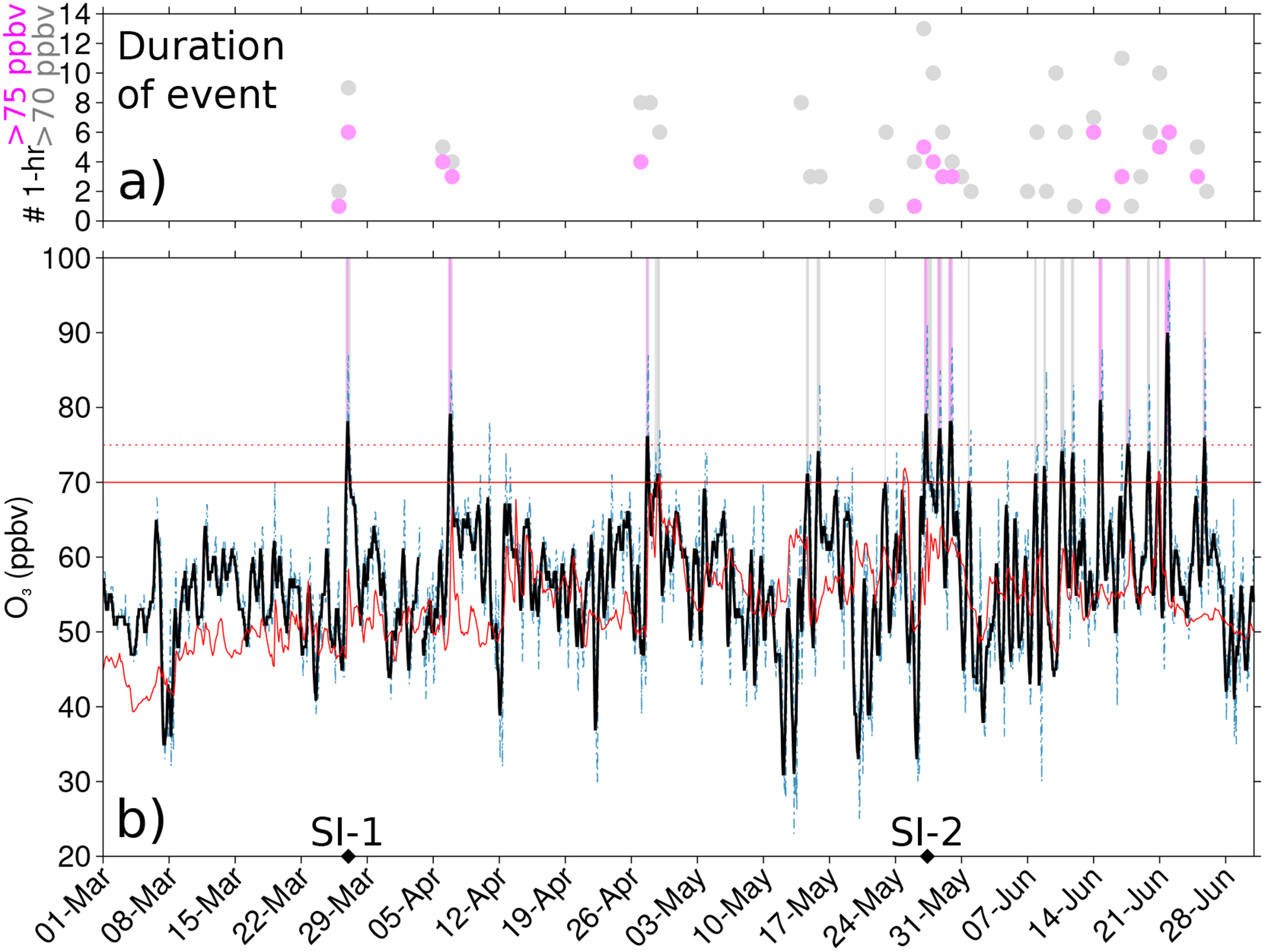
a) Number of hours in an exceedence day (time in UTC) where the RMNP observed hourly average O3 ≥ 75 ppbv (pink circles) and 70 ppbv (grey circles) b) 8-hourly running average O3 (solid black line) and hourly average O3 (dash-dot blue line) from the EPA surface observations at RMNP and the 3-hourly MERRA-2 reanalysis surface O3 at the nearest grid point to RMNP (40°N, 105.625°W; orange line) for 1 March – 30 June 2012 (time in UTC). The exceedence events where the MDA8 O3 ≥ the EPA standard in 2012 (75 ppbv; dotted horizontal red line) are indicated by the vertical pink shading and the events that would be considered exceedences under the new EPA standard (70 ppbv; solid horizontal red line) are indicated by the vertical grey shading. The times of the SI-1 and SI-2 events, corresponding to Figs. 2–4, are indicated by the black diamonds.
At the time of an intrusion, relatively dry air is expected to descend toward the surface behind a cold front [e.g., Bethan et al., 1998; Cooper et al., 2001; Knowland et al., 2015]. Due to the topography, SLP over the Rocky Mountains can be difficult to interpret, however both of the SI case studies occurred when there was a low pressure in the Northern Plains region (Fig. 2a,c). During the SI-1 event, there were two low pressure systems, one in southwest Montana and one in southeast Wyoming (Fig. 2a). The 700 hPa RH was low to the west of a surface trough extending from Wyoming approximately due south into Mexico. For the late spring SI-2 event, a cyclone tracked northeastward into North Dakota with a cold front trailing into western Kansas where it transitions to a stationary front (Fig. 2c). Here, a new low pressure system formed in southeastern Colorado, from which a dry line extends southward through Texas. While relatively low RH is observed by AIRS to the west of the cold front through the Dakotas and Nebraska, there is an even stronger gradient in RH across the dry line (Fig. 2c).
Figure 2.
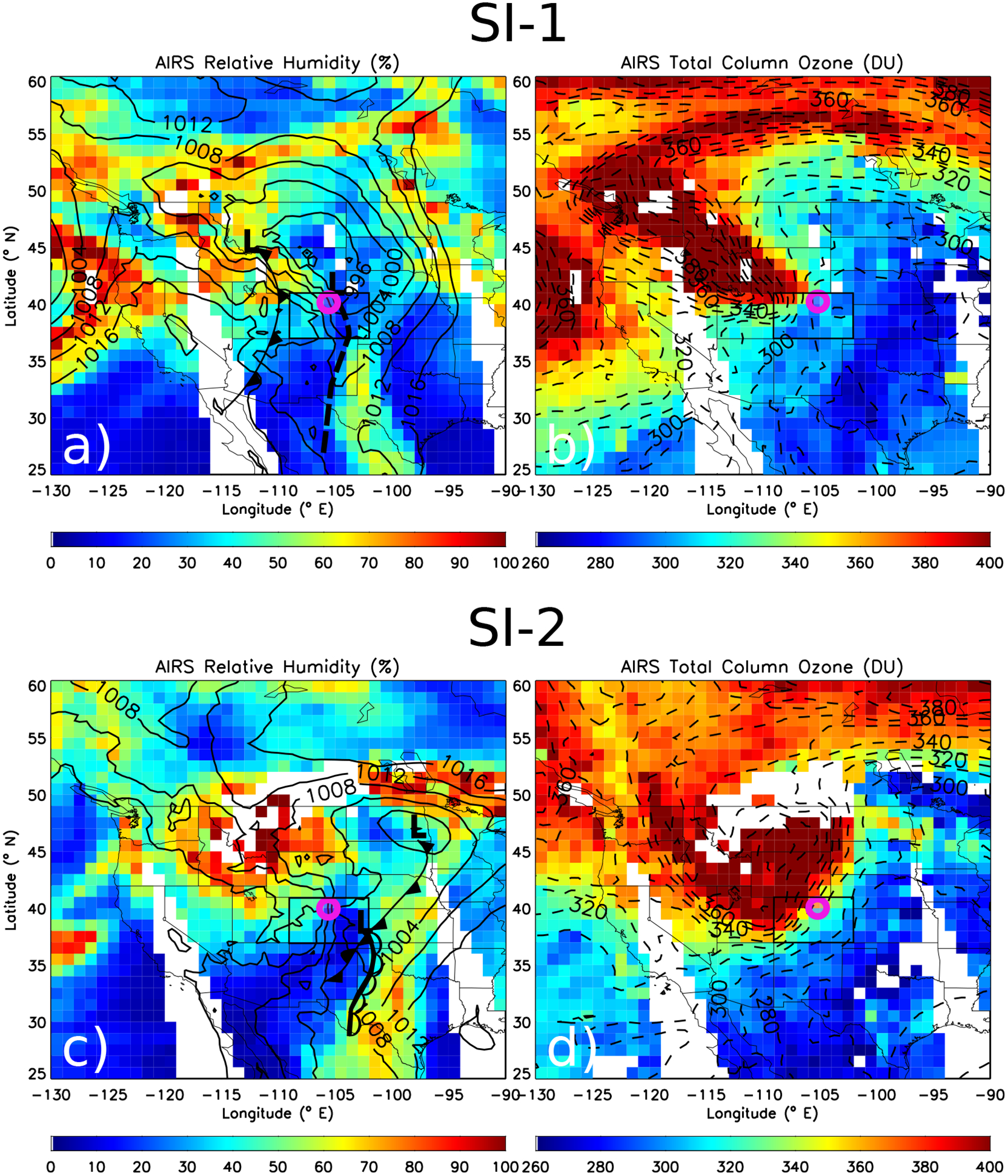
(a,c) AIRS 700 hPa RH (color; %) with MERRA-2 SLP (4 hPa intervals) and (b,d) TCO from AIRS (color; Dobson unit (DU)) and MERRA-2 (dashed; 10 DU intervals) for (a,b) SI-1 and (c,d) SI-2. The approximate location of low pressure centers (“L”) and frontal boundaries – cold front (line with filled triangles (a,c)), surface trough (dashed line (a)), stationary front (filled triangles and half circles on opposite sides of line (c)), dry line (line with open half circles (c)) – are presented from the 18UTC surface analysis (close to 13:30 LT pass) on (a) March 26, 2012 and (c) May 27, 2012 (www.wpc.ncep.noass.gov/archives/web pages/sfc/sfc_archive_maps, Accessed 8 November 2016). Note, not all fronts from the analysis archives have been depicted. The location of RMNP (pink open circle) and the Colorado state border (think black line) are emphasized.
The SI events can be identified by concurrent observations of O3-rich air with the low RH. This can be achieved by focusing on regions where the gradients in TCO are large [Olsen et al., 2000; Ott et al., 2016]. The spatial distributions in AIRS TCO and MERRA-2 TCO at the approximate time of the AIRS observations agree well [Ott et al., 2016], although the MERRA-2 TCO is generally biased low compared to observations in Fig. 2b,d. This aligns with the findings of Wargan et al. [2017] that MERRA-2 TCO in the mid-latitudes was biased low compared to independent TCO measurements from the TOMS (Total Ozone Mapping Spectrometer; Herman et al., 1991) instrument. The maximum TCO – in both AIRS and MERRA-2 – stretches from the Pacific Northwest into the Rocky Mountain states linearly in Fig. 2b and with curvature in Fig. 2d. The location of large TCO gradients in Fig. 2b,d correspond to the low RH regions in Fig. 2a,c; in particular, large TCO gradients in both AIRS and MERRA-2 and low RH are co-located over Colorado (Fig. 2).
We look for further evidence of the SI-1 and SI-2 tropopause folding events in the MERRA-2 reanalysis at the time of maximum O3 at RMNP (Fig. 3). From 300 to 500 hPa over the western USA, there are fine-scale filaments of stratospheric air, specifically high levels of O3 within the 2 PVU contour, which distinguish the SI events from the background (Fig. 3). At the time of maximum hourly O3 observed at RMNP during the SI-1 and SI-2 events, the SI-1 is linear – stretching from Vancouver Island, Canada to the Wyoming-Colorado border – as opposed to the curved SI-2 from Washington down to Arizona and back to Montana (400 hPa, Fig. 3). Both SI events are a result of a cut-off low (COL) near the west coast of the USA in the days prior to the O3 exceedences (not shown). Prior to the exceedence at RMNP as a result of SI-1, the tropopause fold rotates around the COL and at 500 hPa has a hooked shape off the coast of California (not shown) before becoming deformed and elongated – impacting RMNP – as the center of vorticity moves east and the western portion is being pulled west as a consequence of an Aleutian low (Fig. 3a–d). The hook shape of the SI-2 led to the longer period of high O3 (≥ 75 ppbv) at RMNP compared to the duration of high O3 observations associated with SI-1; as the SI-2 fold continued to rotate over the western USA at the end of May, there was continued draw down of stratospheric air toward the surface over the area, unlike the SI-1 event which was steered to the northeast as it decayed. It is worth noting that the tropospheric background levels of MERRA-2 O3 are qualitatively consistent with a seasonal increase in photochemical production from March (Fig. 3a–d) to May (Fig. 3e–h).
Figure 3.
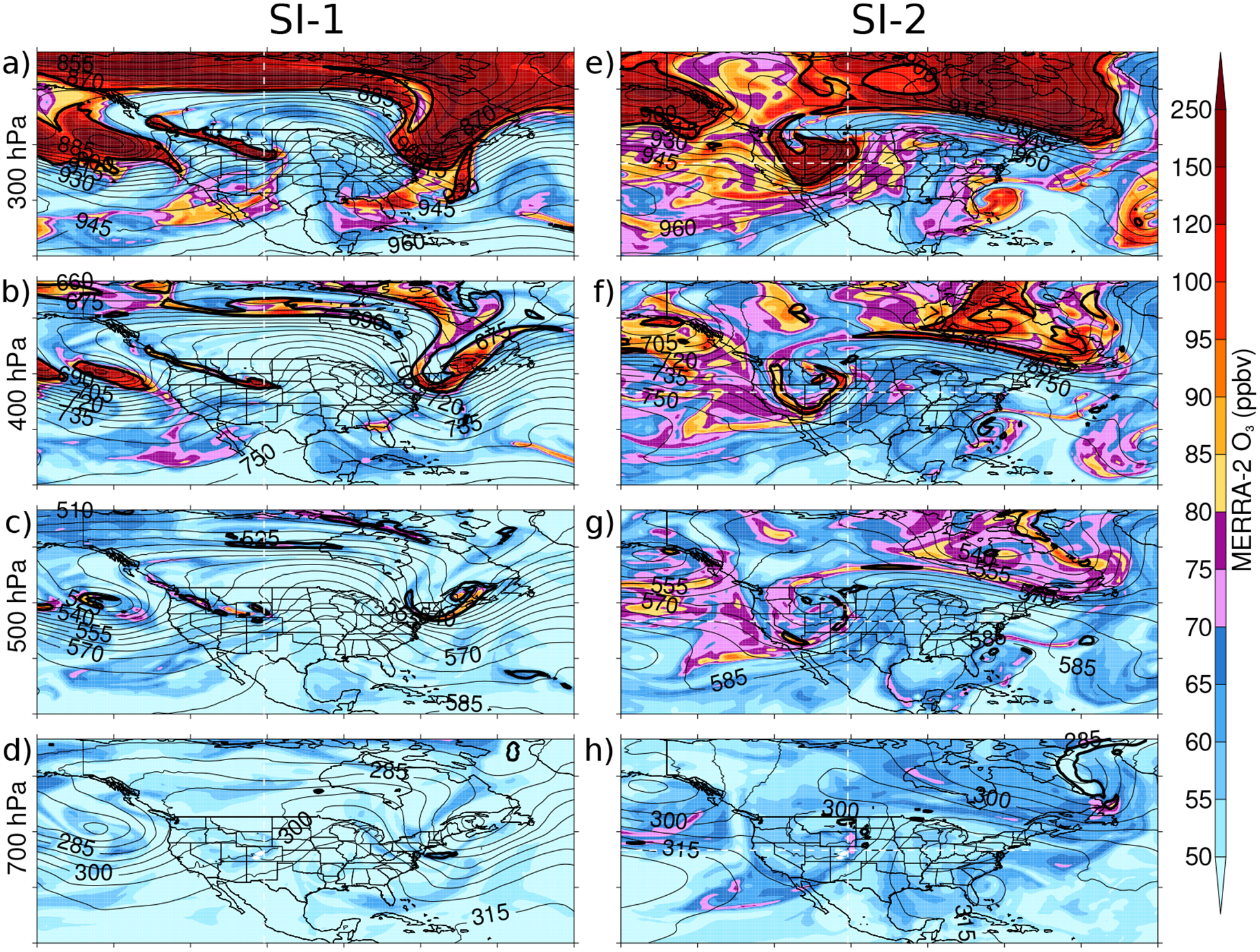
O3 distribution (color; 5 ppbv increments up to 100 ppbv and increment size increases above 100 ppbv), geopotential height (thin black contours; 5 dam intervals) and dynamical tropopause (2 PVU isosurface; thick black contour) on 300 (a,e), 400 (b,f), 500 (c,g) and 700 hPa surfaces (d,h) corresponding to the time of maximum O3 observations at RMNP during the SI-1 event (March 27, 2012 00UTC; a-d) and the SI-2 event (May 27, 2012 09UTC; e-h). Light and dark pink color intervals highlight the previous and current EPA O3 standard, respectively. The white dashed lines correspond to transects in Fig. 4.
The intrusion of air from the stratosphere into the troposphere is captured in vertical transects for the SI events in the MERRA-2 reanalysis dataset and supported by the additional GEOS-5 CO and a fraction of stratospheric air tracer (STFR) data (Fig. 4). In the N-S transect through SI-1, the dynamical tropopause and high O3 (> 85 ppbv, Fig. 4ab; > 40% STFR, Fig. 4c) reached altitudes as low as ~600 hPa, and elevated O3 (> 55 ppbv) reached the surface. Relatively dry air is found within the tropopause fold and in the troposphere to the south of the fold (RH < 30 %, Fig. 4b). The low CO (< 110 ppbv, Fig. 4d) reached 500 hPa within the tropopause fold; however, since the gradient in CO at the base of the fold is less than the gradient of O3, the influence of stratospheric CO was lost due to mixing with tropospheric air characterized by higher CO mixing ratios. A strong jet at 350 hPa (u > 50 m s−1, Fig. 4e) connects down to the surface. There is also a clear frontal boundary on the north-side of the fold extending from an upper-level front (indicated by tight isotherms, Fig. 4a–e) down to the surface with strong descent (ω > 80 hPa h−1, white contours, Fig. 4a) and strong ascent (ω < −80 hPa h−1, black contours, Fig. 4a).
Figure 4.
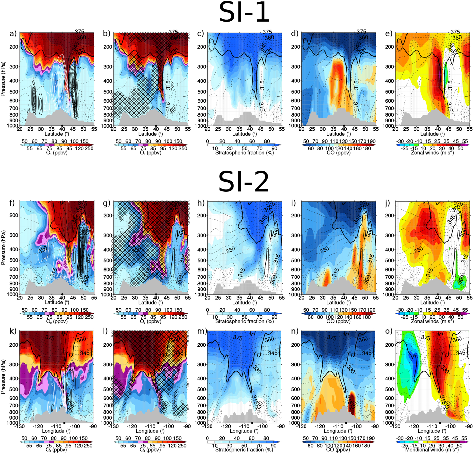
Vertical transects of (a-e) the SI-1 event and (f-o) the SI-2 event taken at the times of maximum O3 observation at (a-j) 105.625°W from 20°-55°N over RMNP (black dot, 40°N) and (k-o) 40°N from 130°-90°W over RMNP (black dot, 105.625°W). O3 (a,b,f,g,k,l; ppbv), Stratospheric fraction (c,h,m; %), CO (d,i,n; ppbv), Zonal winds (e,j; m s−1) and Meridional winds (o; m s−1) are all shown in color with θe (dashed contour lines, 5 K intervals) and the isosurface of 2 PVU (thick black contour). In addition, ω (a,f,k; solid contour lines, 10 hPa h−1 intervals, with white contours for descent and black contours for ascent) and RH (b,g,l; hatching < 30%) are drawn. Orography indicated by grey region.
Both N-S and West-East (W-E) transects are shown for the SI-2 case study (Fig. 4f–o). Although the N-S transect is shown to be just on the eastern edge of the tropopause fold (Fig. 3e–h) and the tropopause does not appear to be depressed below 350 hPa over RMNP (Fig. 4f–j), there are still strong indicators of a fold in the region. Specifically, between 35° to 45°N, there are increased levels of O3 reaching the surface (> 65 ppbv, Fig. 4f,g) within an area marked by strong descent (ω > 60 hPa h−1, Fig. 4f), low humidity (RH < 30 % south of 45°N, Fig. 4g), large STFR (> 60 % at 600 hPa, Fig. 4h), and low CO (< 110 ppbv, Fig. 4i). The frontal boundary can be identified by the large gradients of ω and θe to the north of RMNP. This transect highlights the ascent ahead of the front (reaching up to ~200 hPa at 50°N, maximum ω < −120 hPa h−1 at 400 hPa) and to a lesser extent the descent behind the front (Fig. 4f).
Due to the curvature of the SI-2 fold, the W-E transect intersects both sides of the hook as seen at 400 hPa in Fig. 3f. The W-E transect captures the tropopause fold at 105°W over RMNP reaching 550 hPa as well as the western portion of the fold reaching below 400 hPa at 120°W (Fig. 4k–o). Figure 4o shows the strong jet on both sides of the curved tropopause fold (v > 40 m s−1 at 105°W and v < −30 m s−1 at 120°W). The front above RMNP is also seen in this transect by the large gradients in both ω (Fig. 4k) and θe (Fig. 4k–o). Specifically, isentropic descent above RMNP brings dry, O3-rich air from the stratosphere towards the surface (O3 > 80 ppbv and STFR > 70 % at 600 hPa, O3 > 65 ppbv at surface, Fig. 4k–m). It is interesting to note that low CO (< 110 ppbv, Fig. 4n) is simulated to reach the surface at RMNP, despite the large CO values to the east emitted by a nearby fire. Biomass burning emissions used in the GEOS-5 simulation of CO follow the Quick Fire Emission Dataset (QFED) version 2.4r6 which is based on MODIS satellite fire radiative power (FRP) [Darmenov and da Silva, 2015].
4. Conclusions
Stratospheric intrusions have been the interest of decades of research, especially for the potential influence on ground-level O3 concentrations. However, until recently, the fine-scale nature of the O3 filaments have been misrepresented in models and reanalyses, as the features of an SI are best identified in horizontal resolutions of 50 km or smaller [Büker et al., 2005; Lin et al., 2012; Ott et al., 2016]. For this reason, and likely because reanalysis O3 corresponds better with independent observations in the stratosphere than in the troposphere [Dragani, 2011; Wargan et al., 2015, 2017], there are very few studies of stratosphere-to-troposphere transport which use reanalysis O3 [Škerlak et al., 2014; Zanis et al., 2014; Knowland et al., 2015, 2017; Ott et al., 2016; Ryoo et al., 2017]. NASA’s MERRA-2 reanalysis is such a high-resolution dataset, which benefits from assimilated O3 to present O3 on the same spatiotemporal resolution as the meteorology. Here, two case study examples of SI events which were known to impact surface O3 air quality are examined. The SI events are diagnosed by the folding of the tropopause under the jet stream and subsequent isentropic descent of dry, O3-rich/CO-poor stratospheric air towards the surface using the MERRA-2 reanalysis in combination with surface O3 and satellite observations and GEOS-5 simulated CO and a stratospheric tracer. We show that MERRA-2, a publicly-available dataset, can be used in scientific studies to identify SIs by both atmospheric dynamics and composition. This is a proof of concept study opening the door to detailed multi-year analyses of stratospheric intrusions over the USA and worldwide. Though the MERRA-2 reanalysis tends to underestimate the magnitude of surface O3 during the SIs [see also Ott et al., 2016], the combination of meteorological variables and O3 for a relatively long period of time to within a few weeks of present time may provide a valuable and unique tool for air quality managers [Kaldunski et al., 2017] and scientific studies of stratospheric intrusions.
It is important to be able to identify the differences in anthropogenic and natural sources of O3, especially on exceedence days. Since the GEOS-5 model used to produce MERRA-2 does not simulate full O3 chemistry in the troposphere, we are unable to determine the influence of stratospheric O3 on surface concentrations separate from photochemically-produced O3, especially in late spring/early summer. The impact of photochemically-produced O3 on total O3 later in the spring will be explored in more detail using the GEOS-5 chemistry climate model in a future publication. Yet this study presents strong evidence that the MERRA-2 reanalysis can be used in the identification of SIs.
Key Points:
NASA’s MERRA-2 reanalysis is a publicly-available, high resolution (~50 km) dataset
The MERRA-2 reanalysis, with assimilated O3, captures the fine-scale features of stratospheric intrusions known to impact surface air quality
The combination of meteorological variables and O3 may provide a valuable and unique tool for air quality managers
Acknowledgments
K. Emma Knowland’s analysis of MERRA-2 was supported through GMAO core funding administered by NASA’s Modeling, Analysis, and Prediction Program. Implementation of STFR in GEOS-5 was funded by NASA’s Atmospheric Composition Campaign Data Analysis and Modeling program. The MERRA-2reanalysis data and the AIRS satellite data (AIRX3STD V006) are available through the NASA GES DISC online archive (https://disc.gsfc.nasa.gov/). Tables of the hourly and 8-hourly average O3 observations are available to download on the EPA’s website (http://aqsdr1.epa.gov/aqsweb/aqstmp/airdata/download files.html). The authors would like to acknowledge Brad Weir for providing the GEOS-5 simulation of CO. The GEOS-5 CO and STFR data will be provided upon request by Lesley Ott. The authors would like to thank Pat Reddy for providing the initial list of SI candidates in 2012 and Richard Payton for amassing the list of stratospheric intrusions from the EPA AQS database.
References
- AIRS Science Team/Joao Texeira (2013), AIRS/Aqua L3 Daily Standard Physical Retrieval (AIRS+AMSU) 1 degree × 1 degree V006, Greenbelt, MD, USA, Goddard Earth Sciences Data and Information Services Center (GES DISC), Accessed 19 September 2016, doi:DOI: 10.5067/AQUA/AIRS/DATA301. [DOI] [Google Scholar]
- Aumann HH, Chahine MT, Gautier C, Goldberg MD, Kalnay E, McMillin LM, Revercomb H, Rosenkranz PW, Smith WL, Staelin DH, Strow LL, and Susskind J (2003), AIRS/AMSU/HSB on the Aqua Mission: Design, Science Objectives, Data Products, and Processing Systems, IEEE Trans. Geosci. Remote Sens, 41 (2), 253–264, doi: 10.1109/TGRS.2002.808356. [DOI] [Google Scholar]
- Bader M, Forbes G, Grant J, Lilley R, and Waters A (1995), Images of weather forecasting: A practical guide for interpreting satellite and radar imagery, Cambridge University Press. [Google Scholar]
- Baylon PM, Ja e DA, Pierce RB, and Gustin MS (2016), Interannual Variability in Baseline Ozone and Its Relationship to Surface Ozone in the Western U.S., Environ. Sci. Tech, 50 (6), 2994–3001, doi: 10.1021/acs.est.6b00219,. [DOI] [PubMed] [Google Scholar]
- Bethan S, Vaughan G, Gerbig C, Volz-Thomas A, Richer H, and Tiddeman DA (1998), Chemical air mass differences near fronts, J. Geophys. Res, 103 (D11), 13,413–13,434, doi: 10.1029/98JD00535. [DOI] [Google Scholar]
- Bosilovich M, Akella S, Coy L, Cullather R, Draper C, Gelaro R, Kovach R, Liu Q, Molod A, Norris P, Wargan K, Chao W, Reichle R, Takacs L, Vikhliaev Y, Bloom S, Collow A, Firth S, Labow G, Partyka G, Pawson S, Reale O, Schubert S, and Suarex M (2015), MERRA-2: Initial Evaluation of the Climate, NASA/TM–2015–104606, 43, 139pp. [Google Scholar]
- Bosilovich MG, Lucchesi R, and Suarez M (2016), MERRA-2: File specification GMAO Office Note No. 9 (Version 1.1), Available at: http://gmao.gsfc.nasa.gov/pubs/docs/Bosilovich785.pdf (last access: 20 June 2016).
- Browning K (1997), The dry intrusion perspective of extra-tropical cyclone development, Meteorol. Appl, 4 (4), 317–324. [Google Scholar]
- Büker ML, Hitchman MH, Tripoli GJ, Pierce RB, Browell EV, and Avery MA (2005), Resolution dependence of cross-tropopause ozone transport over east Asia, J. Geophys. Res, 110 (D3), doi: 10.1029/2004JD004739, D03107. [DOI] [Google Scholar]
- Carlson TN (1991), Mid-latitude weather systems, New York, NY (United States); Routledge, Chapman Hall, Inc. [Google Scholar]
- Chahine MT, Pagano TS, Aumann HH, Atlas R, Barnet C, Blaisdell J, Chen L, Divakarla M, Fetzer EJ, Goldberg M, Gautier C, Granger S, Hannon S, Irion FW, Kakar R, Kalnay E, Lambrigtsen BH, Lee S-Y, Marshall JL, McMillan WW, McMillin L, Olsen ET, Revercomb H, Rosenkranz P, Smith WL, Staelin D, Strow LL, Susskind J, Tobin D, Wolf W, and Zhou L (2006), AIRS: Improving Weather Forecasting and Providing New Data on Greenhouse Gases, Bull. Am. Meteorol. Soc, 87 (7), 911–926, doi: 10.1175/BAMS-87-7-911. [DOI] [Google Scholar]
- Cooper O, Forster C, Parrish D, Dunlea E, Höbler G, Fehsenfeld F, Holloway J, Oltmans S, Johnson B, Wimmers A, and Horowitz L (2004), On the life cycle of a stratospheric intrusion and its dispersion into polluted warm conveyor belts, J. Geophys. Res, 109 (D23), doi: 10.1029/2003JD004006. [DOI] [Google Scholar]
- Cooper O, Moody J, Parrish D, Trainer M, Ryerson T, Holloway J, Hubler G, Fehsenfeld F, Oltmans S, and Evans M (2001), Trace gas signatures of the airstreams within North Atlantic cyclones: Case studies from the North Atlantic Regional Experiment (NARE ‘97) aircraft intensive, J. Geophys. Res, 106 (D6), 5437–5456, doi: 10.1029/2000JD900574, 2nd AGU Chapman Conference on Water Vapor in the Climate System, Potomac, Maryland, OCT 12–15, 1999. [DOI] [Google Scholar]
- Danielsen EF (1968), Stratospheric-tropospheric exchange based on radioactivity, ozone and potential vorticity, J. Atmos. Sci, 25 (3), 502–518. [Google Scholar]
- Danielsen EF (1980), Stratospheric source for unexpectedly large values of ozone measured over the Pacific Ocean during Gametag, August 1977, J. Geophys. Res, 85 (C1), 401–412, doi: 10.1029/JC085iC01p00401. [DOI] [Google Scholar]
- Danielsen EF, and Mohnen VA (1977), Project dustorm report: ozone transport, in situ measurements, and meteorological analyses of tropopause folding, J. Geophys. Res, 82 (37), 5867–5877, doi: 10.1029/JC082i037p05867. [DOI] [Google Scholar]
- Darmenov A, and da Silva A (2015), The Quick Fire Emissions Dataset (QFED): Documentation of versions 2.1, 2.2 and 2.4, Tech. rep, NASA/TM2015104606, Vol. 38. [Google Scholar]
- Dragani R (2011), On the quality of the ERA-Interim ozone reanalyses: comparisons with satellite data, Q. J. R. Meteorol. Soc, 137 (658), 1312–1326, doi: 10.1002/qj.821. [DOI] [Google Scholar]
- EPA AirData (2016), https://aqsdr1.epa.gov/aqsweb/aqstmp/airdata/hourly442012012.zip, Last Assessed: 14 September 2016.
- Fischer H, Wienhold FG, Hoor P, Bujok O, Schiller C, Siegmund P, Ambaum M, Scheeren HA, and Lelieveld J (2000), Tracer correlations in the northern high latitude lowermost stratosphere: Influence of cross-tropopause mass exchange, Geophys. Res. Lett, 27 (1), 97–100, doi: 10.1029/1999GL010879. [DOI] [Google Scholar]
- Gelaro R, McCarty W, Surez MJ, Todling R, Molod A, Takacs L, Randles C, Darmenov A, Bosilovich MG, Reichle R, Wargan K, Coy L, Cullather R, Draper C, Akella S, Buchard V, Conaty A, da Silva A, Gu W, Kim G-K, Koster R, Lucchesi R, Merkova D, Nielsen JE, Partyka G, Pawson S, Putman W, Rienecker M, Schubert SD, Sienkiewicz M, and Zhao B (2017), The Modern-Era Retrospective Analysis for Research and Applications, Version 2 (MERRA-2), J. Climate, 30 (14), 5419–5454, doi: 10.1175/JCLI-D-16-0758.1. [DOI] [PMC free article] [PubMed] [Google Scholar]
- GMAO (2015a), MERRA-2 inst3 3d asm Np: 3d,3-Hourly,Instantaneous,Pressure-Level,Assimilation,Assimilated Meteorological Fields V5.12.4, Greenbelt, MD, USA, Goddard Space Flight Center Distributed Active Archive Center (GSFC DAAC), Accessed 4/9/2016, doi: 10.5067/QBZ6MG944HW0. [DOI] [Google Scholar]
- GMAO (2015b), MERRA-2 tavg1 2d slv Nx: 2d,1-Hourly,Time-Averaged,Single-Level,Assimilation,Single-Level Diagnostics V5.12.4, Greenbelt, MD, USA: Goddard Space Flight Center Distributed Active Archive Center (GSFC DAAC), Accessed 11/8/2016, doi: 10.5067/VJAFPLI1CSIV. [DOI] [Google Scholar]
- GMAO (2015c), MERRA-2 tavg1 2d chm Nx: 2d,1-Hourly,Time-Averaged,Single-Level,Assimilation,Carbon Monoxide and Ozone Diagnostics V5.12.4, Greenbelt, MD, USA: Goddard Space Flight Center Distributed Active Archive Center (GSFC DAAC), Accessed 11/8/2016, doi: 10.5067/3RQ5YS674DG. [DOI] [Google Scholar]
- GMAO (2015d), MERRA-2 inst3 3d asm Nv: 3d,3-Hourly,Instantaneous,Model-Level,Assimilation,Assimilated Meteorological Fields V5.12.4, Greenbelt, MD, USA, Goddard Space Flight Center Distributed Active Archive Center (GSFC DAAC), Accessed 4/10/2017, doi: 10.5067/WWQSXQ8IVFW8. [DOI] [Google Scholar]
- Holton JR, Haynes PH, McIntyre ME, Douglass AR, Rood RB, and Pfister L (1995), Stratosphere-troposphere exchange, Rev. Geophys, 33 (4), 403–439, doi: 10.1029/95RG02097. [DOI] [Google Scholar]
- Hoskins B, and Hodges K (2002), New perspectives on the Northern Hemisphere winter storm tracks, J. Atmos. Sci, 59 (6), 1041–1061, doi:. [DOI] [Google Scholar]
- James P, Stohl A, Forster C, Eckhardt S, Seibert P, and Frank A (2003), A 15-year climatology of stratosphere–troposphere exchange with a Lagrangian particle dispersion model 2. Mean climate and seasonal variability, J. Geophys. Res, 108 (D12), doi: 10.1029/2002JD002639, 8522. [DOI] [Google Scholar]
- Kaldunski B, Pierce B, and Holloway T (2017), When Stratospheric Ozone Hits Ground-level Regulation: Exceptional Events in Wyoming, Bull. Amer. Meteor. Soc, 98 (5), 889–892, doi: 10.1175/BAMS-D-14-00133.1. [DOI] [Google Scholar]
- Knowland KE, Doherty RM, and Hodges KI (2015), The effects of springtime mid-latitude storms on trace gas composition determined from the MACC reanalysis, Atmos. Chem. Phys, 15 (6), 3605–3628, doi: 10.5194/acp-15-3605-2015. [DOI] [Google Scholar]
- Knowland KE, Doherty RM, Hodges KI, and Ott LE (2017), The influence of mid-latitude cyclones on European background surface ozone, Atmos. Chem. Phys. Disc, 2017, 1–39, doi: 10.5194/acp-2017-318. [DOI] [PMC free article] [PubMed] [Google Scholar]
- Krzyzanowski M, and Cohen A (2008), Update of WHO air quality guidelines, Air Qual. Atmos. Health, 1, 7–13, doi: 10.1007/s11869-008-0008-9. [DOI] [Google Scholar]
- Langford A, Sen C, II RA, Brioude J, Cooper O, Holloway J, Lin M, Marchbanks R, Pierce R, Sandberg S, Weickmann A, and Williams E (2015), An overview of the 2013 Las Vegas Ozone Study (LVOS): Impact of stratospheric intrusions and long-range transport on surface air quality, Atmos. Environ, 109, 305–322, doi: 10.1016/j.atmosenv.2014.08.040. [DOI] [Google Scholar]
- Langford AO, Masters CD, Pro tt MH, Hsie E-Y, and Tuck AF (1996), Ozone measurements in a tropopause fold associated with a cut-off low system, Geophys. Res. Lett, 23 (18), 2501–2504, doi: 10.1029/96GL02227. [DOI] [Google Scholar]
- Langford AO, Aikin KC, Eubank CS, and Williams EJ (2009), Stratospheric contribution to high surface ozone in Colorado during springtime, Geophys. Res. Lett, 36 (12), doi: 10.1029/2009GL038367, l12801. [DOI] [Google Scholar]
- Langford AO, Brioude J, Cooper OR, Sen CJ, Alvarez RJ, Hardesty RM, Johnson BJ, and Oltmans SJ (2012), Stratospheric influence on surface ozone in the Los Angeles area during late spring and early summer of 2010, J. Geophys. Res, 117 (D21), doi: 10.1029/2011JD016766, D00V06. [DOI] [Google Scholar]
- Lefohn AS, Wernli H, Shadwick D, Limbach S, Oltmans SJ, and Shapiro M (2011), The importance of stratospheric–tropospheric transport in affecting surface ozone concentrations in the western and northern tier of the United States, Atmos. Environ, 45 (28), 4845–4857, doi: 10.1016/j.atmosenv.2011.06.014. [DOI] [Google Scholar]
- Levelt PF, van den Oord GHJ, Dobber MR, Malkki A, Visser H, de Vries J, Stammes P, Lundell JOV, and Saari H (2006), The ozone monitoring instrument, IEEE Trans. Geosci. Remote Sens, 44 (5), 1093–1101, doi: 10.1109/TGRS.2006.872333. [DOI] [Google Scholar]
- Lin M, Fiore AM, Cooper OR, Horowitz LW, Langford AO, Levy H, Johnson BJ, Naik V, Oltmans SJ, and Sen CJ (2012), Springtime high surface ozone events over the western United States: Quantifying the role of stratospheric intrusions, J. Geophys. Res, 117 (D21), doi: 10.1029/2012JD018151. [DOI] [Google Scholar]
- Lin M, Horowitz LW, Oltmans SJ, Fiore AM, and Fan S (2014), Tropospheric ozone trends at Mauna Loa Observatory tied to decadal climate variability, Nat. Geosci, 7 (2), 136–143. [Google Scholar]
- Lin M, Fiore AM, Horowitz LW, Langford AO, Oltmans SJ, Tara-sick D, and Rieder HE (2015), Climate variability modulates western US ozone air quality in spring via deep stratospheric intrusions, Nat. Commun, 6, doi: 10.1038/ncomms8105. [DOI] [PMC free article] [PubMed] [Google Scholar]
- Lovill JE (1970), The structure of gravity waves as determined simultaneously by ozone, temperature, and satellite data, Archs. Met. Geoph. Biokl. Ser. A, 19, 13–28. [Google Scholar]
- U.S. Environmental Protection Agency (2015), National Ambient Air Quality Standards for Ozone; Final Rule, Federal Register, 80 (206), 65,292–65,468. [Google Scholar]
- McCarty W, Coy L, Gelaro R, Huang A, Merkova D, Smith E, Sienkiewicz M, and Wargan K (2016), MERRA-2 Input Observations: Summary and Assessment, NASA/TM–2016–104606, 46, 64pp. [Google Scholar]
- McClain EP (1960), SOME EFFECTS OF THE WESTERN CORDILLERA OF NORTH AMERICA OF CYCLONIC ACTIVITY, J. Meteorol, 17 (2), 104–115, doi:. [DOI] [Google Scholar]
- Monks PS (2000), A review of the observations and origins of the spring ozone maximum, Atmos. Environ, 34 (21), 3545–3561. [Google Scholar]
- Nath D, Chen W, Graf H-F, Lan X, Gong H, Nath R, Hu K, and Wang L (2016), Subtropical Potential Vorticity Intrusion Drives Increasing Tropospheric Ozone over the Tropical Central Pacific, Scientific Reports, 6 (21370), doi: 10.1038/srep21370. [DOI] [PMC free article] [PubMed] [Google Scholar]
- Nieto R, Sprenger M, Wernli H, Trigo RM, and Gimeno L (2008), Identification and Climatology of Cut-off Lows near the Tropopause, Annals of the New York Academy of Sciences, 1146 (1), 256–290, doi: 10.1196/annals.1446.016. [DOI] [PubMed] [Google Scholar]
- Olsen MA, Gallus WA, Stanford JL, and Brown JM (2000), Fine-scale comparison of TOMS total ozone data with model analysis of an intense Midwestern cyclone, J. Geophys. Res, 105 (D16), 20,487–20,495, doi: 10.1029/2000JD900205. [DOI] [Google Scholar]
- Ott L, Duncan B, Pawson S, Colarco P, Chin M, Randles C, Diehl T, and Nielsen E (2010), Influence of the 2006 Indonesian biomass burning aerosols on tropical dynamics studied with the GEOS-5 AGCM, J. Geophys. Res, 115 (D14), doi: 10.1029/2009JD013181, d14121. [DOI] [Google Scholar]
- Ott LE, Duncan BN, Thompson AM, Diskin G, Fasnacht Z, Langford AO, Lin M, Molod AM, Nielsen JE, Pusede SE, Wargan K, Weinheimer AJ, and Yoshida Y (2016), Frequency and impact of summertime stratospheric intrusions over Maryland during DISCOVER-AQ (2011): New evidence from NASA’s GEOS-5 simulations, J. Geophys. Res, 121 (7), 3687–3706, doi: 10.1002/2015JD024052. [DOI] [PMC free article] [PubMed] [Google Scholar]
- Palmén E, and Newton CW (1969), Atmospheric circulation systems: their structure and physical interpretation, 603 pp., Academic Press, New York. [Google Scholar]
- Reutter P, Škerlak B, Sprenger M, and Wernli H (2015), Stratosphere–troposphere exchange (STE) in the vicinity of North Atlantic cyclones, Atmos. Chem. Phys, 15 (19), 10,939–10,953, doi: 10.5194/acp-15-10939-2015. [DOI] [Google Scholar]
- Ryoo J-M, Johnson MS, Iraci LT, Yates EL, and Gore W (2017), Investigating sources of ozone over california using ajax airborne measurements and models: Assessing the contribution from long-range transport, Atmos. Environ, 155, 53–67, doi: 10.1016/j.atmosenv.2017.02.008. [DOI] [Google Scholar]
- Scherrer SC, Croci-Maspoli M, Schwierz C, and Appenzeller C (2006), Two-dimensional indices of atmospheric blocking and their statistical relationship with winter climate patterns in the Euro-Atlantic region, Int. J. Climatol, 26 (2), 233–249, doi: 10.1002/joc.1250. [DOI] [Google Scholar]
- Shapiro M (1980), Turbulent mixing within tropopause folds as a mechanism for the exchange of chemical constituents between the stratosphere and troposphere, J. Atmos. Sci, 37 (5), 994–1004. [Google Scholar]
- Shapiro MA (1974), A Multiple Structured Frontal Zone-Jet Stream System as Revealed by Meteorologically Instrumented Aircraft, Mon. Wea. Rev, 102 (3), 244–253, doi:. [DOI] [Google Scholar]
- Sprenger M, and Wernli H (2003), A northern hemispheric climatology of cross-tropopause exchange for the ERA15 time period (1979–1993), J. Geophys. Res, 108 (D12), doi: 10.1029/2002JD002636. [DOI] [Google Scholar]
- Stohl A, and Trickl T (1999), A textbook example of long-range transport: Simultaneous observation of ozone maxima of stratospheric and North American origin in the free troposphere over Europe, J. Geophys. Res, 104 (D23), 30,445–30,462, doi: 10.1029/1999JD900803. [DOI] [Google Scholar]
- Stohl A, Wernli H, James P, Bourqui M, Forster C, Liniger MA, Seibert P, and Sprenger M (2003), A new perspective of stratosphere-troposphere exchange, Bull. Am. Meteorol. Soc, 84 (11), 1565–1573. [Google Scholar]
- Susskind J, Barnet C, Blaisdell J, Iredell L, Keita F, Kouvaris L, Molnar G, and Chahine M (2006), Accuracy of geophysical parameters derived from Atmospheric Infrared Sounder/Advanced Microwave Sounding Unit as a function of fractional cloud cover, J. Geophys. Res, 111 (D9), doi: 10.1029/2005JD006272, D09S17. [DOI] [Google Scholar]
- US EPA AQS database (2017), https://www.epa.gov/aqs, Data extracted from the US EPA AQS database, 27 January 2017.
- Škerlak B, Sprenger M, and Wernli H (2014), A global climatology of stratosphere–troposphere exchange using the ERA-Interim data set from 1979 to 2011, Atmos. Chem. Phys, 14 (2), 913–937, doi: 10.5194/acp-14-913-2014. [DOI] [Google Scholar]
- Wargan K, Pawson S, Olsen MA, Witte JC, Douglass AR, Ziemke JR, Strahan SE, and Nielsen JE (2015), The global structure of upper troposphere-lower stratosphere ozone in GEOS-5: A multiyear assimilation of EOS Aura data, J. Geophys. Res, 120 (5), 2013–2036, doi: 10.1002/2014JD022493, 2014JD022493. [DOI] [Google Scholar]
- Wargan K, Labow G, Frith S, Pawson S, Livesey N, and Partyka G (2017), Evaluation of the Ozone Fields in NASAs MERRA-2 Reanalysis, J. Climate, 30 (8), doi: 10.1175/JCLI-D-16-0699.1. [DOI] [PMC free article] [PubMed] [Google Scholar]
- Waters JW, Froidevaux L, Harwood RS, Jarnot RF, Pickett HM, Read WG, Siegel PH, Cofield RE, Filipiak MJ, Flower DA, Holden JR, Lau GK, Livesey NJ, Manney GL, Pumphrey HC, Santee ML, Wu DL, Cuddy DT, Lay RR, Loo MS, Perun VS, Schwartz MJ, Stek PC, Thurstans RP, Boyles MA, Chandra KM, Chavez MC, Chen G-S, Chudasama BV, Dodge R, Fuller RA, Girard MA, Jiang JH, Jiang Y, Knosp BW, LaBelle RC, Lam JC, Lee KA, Miller D, Oswald JE, Patel NC, Pukala DM, Quintero O, Sca DM, Snyder WV, Tope MC, Wagner PA, and Walch MJ (2006), The Earth Observing System Microwave Limb Sounder (EOS MLS) on the Aura Satellite, IEEE Trans. Geosci. Remote Sens, 44 (5), 1075–1092. [Google Scholar]
- Waugh DW, and Polvani LM (2000), Climatology of intrusions into the tropical upper troposphere, Geophys. Res. Lett, 27 (23), 3857–3860, doi: 10.1029/2000GL012250. [DOI] [Google Scholar]
- Wimmers AJ, Moody JL, Browell EV, Hair JW, Grant WB, Butler CF, Fenn MA, Schmidt CC, Li J, and Ridley BA (2003), Signatures of tropopause folding in satellite imagery, J. Geophys. Res, 108 (D4), doi: 10.1029/2001JD001358. [DOI] [Google Scholar]
- Yates EL, Iraci LT, Roby MC, Pierce RB, Johnson MS, Reddy PJ, Tadić JM, Loewenstein M, and Gore W (2013), Airborne observations and modeling of springtime stratosphere-to-troposphere transport over California, Atmos. Chem. Phys, 13 (24), 12,481–12,494, doi: 10.5194/acp-13-12481-2013. [DOI] [Google Scholar]
- Zanis P, Hadjinicolaou P, Pozzer A, Tyrlis E, Dafka S, Mihalopoulos N, and Lelieveld J (2014), Summertime free-tropospheric ozone pool over the eastern Mediterranean/Middle East, Atmos. Chem. Phys, 14 (1), 115–132, doi: 10.5194/acp-14-115-2014. [DOI] [Google Scholar]
- Zhang L, Jacob DJ, Yue X, Downey NV, Wood DA, and Blewitt D (2014), Sources contributing to background surface ozone in the US Intermountain West, Atmos. Chem. Phys, 14 (11), 5295–5309, doi: 10.5194/acp-14-5295-2014. [DOI] [Google Scholar]