Quantitative Interpretation of Solvent Paramagnetic Relaxation for Probing Protein–Cosolute Interactions

Abstract

Protein–small cosolute molecule interactions are ubiquitous and known to modulate the solubility, stability, and function of many proteins. Characterization of such transient weak interactions at atomic resolution remains challenging. In this work, we develop a simple and practical NMR method for extracting both energetic and dynamic information on protein–cosolute interactions from solvent paramagnetic relaxation enhancement (sPRE) measurements. Our procedure is based on an approximate (non-Lorentzian) spectral density that behaves exactly at both high and low frequencies. This spectral density contains two parameters, one global related to the translational diffusion coefficient of the paramagnetic cosolute, and the other residue specific. These parameters can be readily determined from sPRE data, and then used to calculate analytically a concentration normalized equilibrium average of the interspin distance, ⟨r⁻⁶⟩_norm, and an effective correlation time, ${\tau }_{\text{C}},$ that provide measures of the energetics and dynamics of the interaction at atomic resolution. We compare our approach with existing ones, and demonstrate the utility of our method using experimental ¹H longitudinal and transverse sPRE data recorded on the protein ubiquitin in the presence of two different nitroxide radical cosolutes, at multiple static magnetic fields. The approach for analyzing sPRE data outlined here provides a powerful tool for deepening our understanding of extremely weak protein–cosolute interactions.

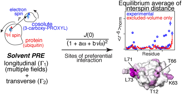
Graphical Abstract

INTRODUCTION

Protein–cosolute interactions play a critical role in protein the current work. stability,^1,2 dynamics,³ function,^4,5 and molecular recognition.^6,7 stability,^1,2 dynamics,³ function,^4,5 and molecular recognition.^6,7 In particular, weak interactions between proteins and small cosolutes (such as urea, ATP, trimethylamine N-oxide, amino acids, etc.) are ubiquitous in biochemical processes within cells.^8,9 For example, one class of small cosolutes known as osmolytes, such as sorbitals and betaines, tend to accumulate in kidney cells to counteract the denaturation effect of urea.^10,11 Recently, osmolytes have also been shown to modulate protein aggregation processes involved in a number of neurodegenerative diseases.^12–15

Despite considerable scientific interest,^9,16–18 the mechanistic details of protein–cosolute interactions are not well established at the molecular level, largely due to their extremely weak and transient nature that are invisible to most biophysical techniques. As a result, molecular details have largely been inferred from theoretical^19–24 and computational^20,25–29 studies.

NMR spectroscopy can potentially report on the energetics and time scale of protein–cosolute interactions.^30–36 In particular, solvent paramagnetic relaxation enhancement (sPRE)^37–42 can directly probe the interaction between between a paramagnetic cosolute and a protein at atomic resolution. A new way of interpreting sPRE data is the subject of the current work.

Even for the simple analytically tractable model where the protein and paramagnetic cosolute are described as hard-spheres with no intermolecular forces between them, analysis and interpretation of the sPRE is difficult and of little practical utility.^43,44 In the absence of intermolecular interactions other than excluded volume, the transverse sPRE relaxation time can be reasonably well described by computing ensemble average distances, ${\langle r^{-6}\rangle }_{\text{norm}}^{\text{exc}}$ (normalized for cosolute concentration) between the unpaired electron on the cosolute and protons on the protein with the distance of closest approach being limited by the protein molecular surface.^41,42,45 The latter is easily calculated directly from atomic coordinates. However, agreement with experiment is poor when preferential protein–cosolute interactions are present⁴² (see Figure S1 of the Supporting Information, SI), which is the main interest of this work.

Here, we propose a simple, but more accurate alternative, based on an approximate non-Lorentzian spectral density function that can be used to fit spectral densities obtained from experimental longitudinal (Γ₁) and transverse (Γ₂) sPRE rates.³⁶ This approach enables one to extract two residue-specific quantities from the experimental sPRE data that characterize paramagnetic cosolute–protein interactions at the atomic level: (i) the cosolute concentration normalized, equilibrium average protein–cosolute interspin distance, ${\langle r^{-6}\rangle }_{\text{norm}},$ and (ii) the effective correlation time ${\tau }_{\text{C}}$ which is a measure of the time-scale of the protein–cosolute interaction. ${\langle r^{-6}\rangle }_{\text{norm}}$ is independent of dynamics and is very sensitive to local intermolecular interactions. In particular, the value of ${\langle r^{-6}\rangle }_{\text{norm}}$ will increase in the presence of an attractive potential and decrease in the presence of a repulsive potential. Both ${\langle r^{-6}\rangle }_{\text{norm}}$ and ${\tau }_{\text{C}}$ are meaningful even when well-defined binding states are not formed, as in the case of weak protein–cosolute interactions. Further, comparison of ${\langle r^{-6}\rangle }_{\text{norm}}^{\text{exc}}$ values calculated directly from a protein structure^41,42,45with the experimentally determined ${\langle r^{-6}\rangle }_{\text{norm}}$ values enables one to ascertain at the atomic level whether the protein–cosolute interactions are attractive or repulsive.

THEORY

Relaxation due to direct dipole–dipole interaction between a proton spin on the protein and the electron spin on the paramagnetic cosolute in an isotropic liquid is described by the time-correlation function C(t) given by:⁴⁶

$$C(t)=4\pi N_{\text{S}}\langle \frac{Y_{2,0}^{*}({\mathrm{\Omega }}^{\text{LF}}(0))}{r^3(0)}\frac{Y_{2,0}({\mathrm{\Omega }}^{\text{LF}}(t))}{r^3(t)}\rangle$$ (1)

where r and ${\mathrm{\Omega }}^{\text{LF}}$ denote the length and orientation of a vector, $\overrightarrow{r},$ between the protein and the cosolute spins in the laboratory frame (see Figure 1). $Y_{2,0}({\mathrm{\Omega }}^{\text{LF}})$ is the spherical harmonic, $Y_{l,m}({\mathrm{\Omega }}^{\text{LF}}),$ with l = 2 and m = 0; N_S is the number of cosolute spins; and the brackets $\langle \rangle$ denote an equilibrium average of all positions and orientations of the protein–cosolute pair. Equation 1 ignores fluctuations of dipole–dipole interactions arising from electron spin relaxation.

Figure 1.

Definition of the interspin vector $\overrightarrow{r}$.

We define the spectral density as the cosine transform of C(t):

$$J(\omega )={\int }_0^{\infty }C(t)\cos (\omega t)\text{d}t$$ (2)

The difference in the longitudinal and transverse relaxation rates of the protein spin in the presence and absence of the paramagnetic cosolute, denoted as Γ₁ and Γ₂,³⁶ respectively, are related to J(ω) by:⁴⁶

$${\mathrm{\Gamma }}_1=\frac{3}{10}{\left(\frac{{\mu }_{\text{o}}}{4\pi }\right)}^2{\hslash }^2{\gamma }_{\text{H}}^2{\gamma }_{\text{e}}^{2}J({\omega }_{\text{H}})$$ (3)

and

$${\mathrm{\Gamma }}_2=\frac{1}{5}{\left(\frac{{\mu }_{\text{o}}}{4\pi }\right)}^2{\hslash }^2{\gamma }_{\text{H}}^2{\gamma }_{\text{e}}^2\left(J(0)+\frac{3}{4}J({\omega }_{\text{H}})\right)$$ (4)

where μ_o is the vacuum permittivity constant divided by 2π; $\hslash$ is Planck’s constant; γ_H and γ_e are the gyromagnetic ratios of the ¹H spin of interest in the protein and the electron spin of the cosolute; and ${\omega }_{\text{H}}/2\pi$ is the Larmor frequency of the proton spins at given spectrometer field. It should be pointed out that eqs 3 and 4 neglect terms involving ω_e as the latter is ∼660 times larger than ω_H, and hence terms containing J(ω_e) and J(ω_H ± ω_e) are negligibly small compared to those with J(0) or J(ω_H). If Γ₁ is measured at n magnetic fields and Γ₂ at one of them, then n + 1 spectral densities can be determined: J(0), J(ω₁), ..., J(ω_n).

In isotropic solution, the correlation function is identical when $Y_{2,0}({\mathrm{\Omega }}^{\text{LF}})$ is replaced in eq 1 by $Y_{2,m}({\mathrm{\Omega }}^{\text{LF}})$ for all values of m.⁴⁷ Consequently, using the addition theorem for spherical harmonics, C(t) can be written as:

$$C(t)=N_{\text{S}}\langle \frac{P_2(\widehat{r}(0)\cdot \widehat{r}(t))}{r^3(0)r{(t)}^3}\rangle$$ (5)

where P₂(x) is the second order Legendre polynomial, and $\widehat{r}$ is a unit vector between the protein and cosolute spins. This expression for C(t) depends on the dot product of $\widehat{r}(0)$ and $\widehat{r}(t),$ and is therefore independent of the reference frame.

From eq 5 it follows that the initial value of the correlation function is given, in general, by:

$$C(0)=N_{\text{S}}\langle r^{-6}\rangle =4\pi n_{\text{S}}{\int }_0^{\infty }\frac{g(r)}{r^4}\text{d}r$$ (6)

where g(r) is the pair correlation function: g(r)/V dr is the probability of finding the protein and cosolute spins at a distance between r and r + dr in volume V; and n_S is the number density (concentration) of the paramagnetic cosolute (i.e., N_S/V). In general, g(r) is related to the potential of the mean force $U(r)$ by $g(r)=\exp (-U(r)/k_{\text{B}}T)$ where k_B is the Boltzmann constant, and T the temperature. It should be emphasized that eq 6 is valid for arbitrary shapes of the protein and cosolute and for arbitrary intermolecular interactions between them.

It is convenient to define a concentration independent equilibrium average:

$${\langle r^{-6}\rangle }_{\text{norm}}=\frac{C(0)}{n_{\text{S}}}=4\pi {\int }_0^{\infty }\frac{g(r)}{r^4}\text{d}r$$ (7)

which has units of m⁻³ instead of m⁻⁶. This average is determined not only by the excluded volume interactions between the protein and cosolute but also by additional site-specific intermolecular forces due to electrostatic and hydrophobic interactions. Let us denote the values of this average calculated considering the excluded volume of the protein and cosolute by ${\langle r^{-6}\rangle }_{\text{norm}}^{\text{exc}}$ which, in practice, can be calculated from the protein coordinates.^41,42,45 Clearly when ${\langle r^{-6}\rangle }_{\text{norm}}$ is larger than ${\langle r^{-6}\rangle }_{\text{norm}}^{\text{exc}}$, local attractive interactions are present, whereas when ${\langle r^{-6}\rangle }_{\text{norm}}$ is smaller than ${\langle r^{-6}\rangle }_{\text{norm}}^{\text{exc}}$, there are local repulsive interactions. Consequently ${\langle r^{-6}\rangle }_{\text{norm}}$ can be used to identify the types of interactions (attractive, no force or repulsive) between the cosolute and individual protons in the protein.

In principle, ${\langle r^{-6}\rangle }_{\text{norm}}$ could be found⁴⁸ if J(ω) were known at all frequencies using the inverse cosine transform of eq 2 at t = 0,

$${\langle r^{-6}\rangle }_{\text{norm}}=\frac{2}{n_{\text{S}}\pi }{\int }_0^{\infty }J(\omega )\text{d}\omega$$ (8)

In practice, J(ω) can only be determined at a small number of frequencies owing to the limited availability of NMR spectrometer fields.

The simplest approximate spectral density, J_approx(ω), is a Lorentzian:

$$J_{\text{approx}}(\omega )=\frac{J(0)}{1+{(\omega {\tau }_{\text{C}})}^2}$$ (9)

If Γ₁ and Γ₂ (and hence J(0) and J(ω)) were measured at a single magnetic field, τ_C could be found uniquely from eq 9,

$${\tau }_{\text{C}}=\sqrt{\frac{J(0)-J(\omega )}{{\omega }^{2}J(\omega )}}\approx \sqrt{\frac{J(0)}{{\omega }^{2}J(\omega )}}$$ (10)

and from eq 8 it follows that,

$${\langle r^{-6}\rangle }_{\text{norm}}=\frac{J(0)}{n_{\text{S}}{\tau }_{\text{C}}}$$ (11)

If data at more fields are available, then ${\tau }_{\text{C}}$ can be found by leastsquares fitting. If only Γ₂ at a single magnetic field is determined for a large number of residues, then the corresponding ${\langle r^{-6}\rangle }_{\text{norm}}$ values can be obtained from eq 11 assuming that ${\mathrm{\Gamma }}_2\propto J(0)(\text{i.e.,}J(\omega )\ll J(0))$ and ${\tau }_{\text{C}}$ is same for all residues. The latter is not generally valid (see Figure S2). The purpose of this work is to do better without significantly complicating the analysis.

For the sPRE, the Lorentzian spectral density is flawed because in the low frequency limit, as a result of translational diffusion, the spectral density behaves as:^{43,44,49–54}

$$\underset{\omega \to 0}{\lim }J(\omega )=J(0)-B\sqrt{\omega }+\dots$$ (12)

where B is a constant. The Lorentzian spectral density, given by eq 9, however, approaches $J(0)$ as ${\omega }^2$ when ω → 0. However, the exact J(ω) behaves like a Lorentzian in the high frequency limit,^43,44,53

$$\underset{\omega \to \infty }{\lim }J(\omega )=A{\omega }^{-2}+\dots$$ (13)

where A is a constant.

According to Sholl⁴⁹ and Fries,⁵⁰ the constant B in eq 12 is independent of intermolecular interactions and is given by:

$$B=\frac{2\sqrt{2}\pi n_{\text{S}}}{9D_{\text{trans}}^{3/2}}$$ (14)

where D_trans is the relative translational diffusion constant of the interacting molecules.

Our approach to the analysis of sPRE data is based on the following ansatz for the spectral density,

$$J_{\text{approx}}(\omega )=\frac{J(0)}{{(1+a\omega +b\sqrt{\omega })}^2}$$ (15)

when a and b are set to:

$$a=\sqrt{J(0)/A}$$ (16)

and,

$$b=\frac{B}{2J(0)}=\frac{\sqrt{2}\pi n_{\text{S}}}{9D_{\mathrm{trans}}^{3/2}J(0)}$$ (17)

The spectral density in eq 15 reproduces the first two terms in the low-frequency expansion of J(ω) (cf. eq 12) and the first term in the high-frequency expansion of J(ω) (cf. eq 13). Here, we will treat a and b as adjustable fitted parameters. a is a site-specific parameter that varies from atom to atom in the protein. The parameter b is also site-specific but is obtained directly from D_trans and the experimental, residue-specific values of J(0) using eq 17. Therefore, we fit the experimental J(ω) data by optimizing a and D_trans.

Once a and b are determined with the spectral density given by eq 15, ${\langle r^{-6}\rangle }_{\text{norm}}$ can be obtained by evaluating the integral in eq 8. We find,

$${\langle r^{-6}\rangle }_{\text{norm}}=\frac{16J(0)}{n_S\pi }\frac{\left(2\left(x_{-}-x_{+}\right)+\left(x_{-}+x_{+}\right)\ln \left(x_{+}/x_{-}\right)\right)}{{\left(x_{-}-x_{+}\right)}^3}$$ (18)

where $x_{\pm }=-b\pm \sqrt{b^2-4a}.$ Once the ${\langle r^{-6}\rangle }_{\text{norm}}$ values are known, we can calculate the effective residue-dependent correlation time ${\tau }_{\text{C}}$ defined as:⁴⁸

$${\tau }_{\text{C}}=\frac{{\int }_0^{\infty }C(t)\text{d}t}{C(0)}=\frac{J(0)}{n_{\text{S}}{\langle r^{-6}\rangle }_{\text{norm}}}$$ (19)

${\tau }_{\text{C}}$ is a measure of the time scale of the fluctuations of the interspin vector $\overrightarrow{r},$ which arise from both translational and rotational diffusion and are influenced by both short and long-range intermolecular interactions. The quantitative interpretation of the physical meaning of ${\tau }_{\text{C}}$ is model dependent (see SI Figure S3).

RESULTS AND DISCUSSION

Validation of the Approximate Spectral Density Function Equation 15 for the Force-Free Model.

The simplest theoretical analysis of intermolecular dipolar relaxation, developed by Hwang⁴³ and Ayant⁴⁴ is based on a “force-free” model which assumes the protein and cosolute are hard-spheres with no intermolecular forces (other than excluded volume) between them. The cosolute and protein spins can be located anywhere in spheres that undergo rotational diffusion independently of one another. The spectral density function for this simple hard-sphere model is given analytically by:⁴⁴

$$\begin{gathered} J(\omega )=\frac{\pi n_s}{6D_{\text{trans}}d}\sum _{l=0}^{\infty }(2l+4)!\sum _{k=0}^l\frac{1}{(2k+1)!(2l-2k+1)!}{\left(\frac{s}{d}\right)}^{2(l-k)} \\ \times {\left(\frac{p}{d}\right)}^{2k}\mathrm{Re}[j_{l+2}({\sigma }_{lk})] \end{gathered}$$ (20)

where

$$j_l(x)=\left(\frac{1}{x^2}\right)\left(\frac{1}{2l-1}-\frac{l+1}{x^2}{\left(1+\frac{l+1}{x}\frac{K_{l+1/2}(x)}{K_{l-1/2}(x)}\right)}^{-1}\right)$$ (21)

$$\tau =d^2/D_{\text{trans}}$$ (22)

$$\frac{1}{{\tau }_{Q,l}}=l(l+1)D_{\text{Rot},Q}$$ (23)

$${\sigma }_{lk}=\sqrt{i\omega \tau +\frac{\tau }{{\tau }_{\text{P},k}}+\frac{\tau }{{\tau }_{\text{S},l-k}}}$$ (24)

K_ν(x) is a modified Bessel function of the second kind of order ν; d is the contact distance between protein and cosolute; s and p are the center-to-spin distances of cosolute and protein, respectively; D_trans is the relative translational diffusion constant; Q in eq 23 is the index for either protein (P) or cosolute (S); and D_Rot,Q is the rotational diffusion constant of the protein or cosolute. For convenience, we denote the rotational correlation times of the protein $({\tau }_{\text{P}})$ and the cosolute $({\tau }_{\text{S}})$ as ${\tau }_{\text{Q},l}$ when l = 2, i.e.,

$$\frac{1}{{\tau }_Q}=6D_{\text{Rot},Q}$$ (25)

where Q is P or S.

To demonstrate the validity of our spectral density given by eq 15, we analyzed a large set of simulated data points using the exact force-free spectra density eq 20 for a range of physically reasonable values of ${\tau }_{\text{P}}$ and ${\tau }_{\text{S}},$ and the results for a representative sample are presented below. For each simulation, we used the Stoke–Einstein relation,

$$D_{\text{trans}}=\frac{k_{\text{B}}T}{6\pi \eta R_{\text{P}}}+\frac{k_{\text{B}}T}{6\pi \eta R_{\text{S}}}$$ (26)

and

$$D_{\text{Rot},Q}=\frac{k_{\text{B}}T}{8\pi \eta {R_Q}^3}$$ (27)

where k_B is the Boltzmann constant; η is the viscosity of the solvent; and R_P and R_S are the hard sphere radii of the protein and cosolute, respectively. We set T = 298 K and η = 8.9 × 10⁻⁴ J s m⁻³ (equal to the viscosity of water at 298 K). For each value of ${\tau }_{\text{P}}$ and ${\tau }_{\text{S}},$ R_P and R_S were back calculated from eqs 25 and 27 and d was set to R_P + R_S. Simulated values of J(ω) at ω = 0, 2π (500 MHz), 2π (800 MHz), and 2π (900 MHz) were generated and fitted to eq 15 optimizing the values of a and D_trans. Comparisons between representative exact spectral densities obtained from eq 20 with ${\tau }_{\text{P}}=3.8\text{ns}$ and ${\tau }_{\text{S}}=39\text{ps}$ and the fits using the approximate spectral density of eq 15 and the single Lorentzian spectral density of eq 9, are shown in Figure 2A and B, respectively. Equation 15 reproduces the exact spectral density essentially perfectly, whereas clear systematic differences are observed for eq 9. The optimized value of D_trans obtained from the fit is 7.3 (±0.1) × 10⁻¹⁰ m² s⁻¹ which is close to the exact value of 8.5 × 10⁻¹⁰ m² s⁻¹. The optimized value of D_trans is slightly underestimated probably due to insufficient number of data points in the low-frequency regime where J(ω) is most sensitive to D_trans (see eq 12). Complete cross-validation in which fitting the Γ₁ values at two fields is used to predict the Γ₁ values at the third field for all three combinations of fields reveal excellent agreement for eq 15 (Figure 2C), but poor agreement for eq 9 (Figure 2D).

Figure 2.

Validation of the approximate spectral density function, eq 15, for hard-sphere protein–cosolute interactions. (A) and (B) comparison of the exact force-free hard-sphere spectral densities (continuous gray lines) calculated using eq 20 with those calculated using either our approximate (eq 15, panel A) or single Lorentzian (eq 9, panel B) spectral density functions (shown as dashed red lines) at several distances of the ¹H spin to the surface of an idealized protein represented by a sphere. The parameters used to generate the exact spectral densities are ${\tau }_{\text{P}}=3.8\text{ns}$ and ${\tau }_{\text{S}}=39\text{ps}$ (corresponding to spheres of radii ∼17 Å and ∼3.5 Å, respectively). The ¹H spin is located within the protein sphere at distances of 1, 2, 3, 4, and 5 Å from the protein surface. The electron spin is located at 1 Å from the surface of the cosolute. The approximate spectral densities obtained using eq 15 superimpose almost exactly on the exact spectral densities calculated using eq 20. The blue circles represent the points from the exact spectral densities used to fit the approximate spectral density functions. (C) and (D) results of complete cross-validation fitting the Γ₁ data at 2 fields using eqs 15 and 9, respectively, and comparing the predicted and exact Γ₁ values at the third field (free data set). Q_free is a measure of agreement between predicted ${\mathrm{\Gamma }}_1^{\text{calc,free}}(i)$ and experimental ${\mathrm{\Gamma }}_1^{\text{obs},\text{free}}(i)$ values for the free data set (i.e., not used in fitting) and:

$${\left\{\sum _i{\left[{\mathrm{\Gamma }}_1^{\text{obs},\text{free}}(i)-{\mathrm{\Gamma }}_1^{\text{calc},\text{free}}(i)\right]}^2/\sum _i{\mathrm{\Gamma }}_1^{\text{obs},\text{free}}{(i)}^2\right\}}^{1/2}$$

Where the summation with index i runs over all data points i at a given field. (E) and (F) ratios of approximate to exact ${\langle r^{-6}\rangle }_{\text{norm}}$ values obtained using eqs 15 and 9, respectively, for 2- and 3-field fits. (G) and (H) correlation plots between exact and approximate ${\langle r^{-6}\rangle }_{\text{norm}}$ values obtained using eqs 15 and 9, respectively, for a range of parameters: ${\tau }_{\text{P}}=2,5,10,$ and $15\text{ns};{\tau }_{\text{S}}=5,25,50,100,$ and $250\text{ps};$ and the ¹H spin located at 2 (red), 4 (green), and 6 (blue) Å from the protein surface. The electron spin is located at the center of the cosolute sphere.

Comparison between the exact ${\langle r^{-6}\rangle }_{\text{norm}}^{\text{exact}}$ values and the approximate ${\langle r^{-6}\rangle }_{\text{norm}}^{\text{approx}}$ obtained with the approximate spectral density functions using both a 3-field fit and three different combinations of 2-field fits, shows excellent agreement for eq 15 (Figure 2E), but poor agreement with systematic deviations for eq 9 (Figure 2F). In addition, the correlation between ${\langle r^{-6}\rangle }_{\text{norm}}^{\text{exact}}$ and ${\langle r^{-6}\rangle }_{\text{norm}}^{\text{approx}}$ for a variety of different ${\tau }_{\text{P}}$ and ${\tau }_{\text{S}},$ values is excellent for eq 15 (Figure 2G) but exhibits clear systematic deviations for eq 9 (Figure 2H).

The impact of 1-field and 2-field fitting on the accuracy of the extracted ${\langle r^{-6}\rangle }_{\text{norm}}^{\text{approx}}$ values is investigated in Figures S4 and S5. In the case of eq 15 there is essentially no difference between 3-field and 2-field fitting, and significant deviations between ${\langle r^{-6}\rangle }_{\text{norm}}^{\text{approx}}$ and ${\langle r^{-6}\rangle }_{\text{norm}}^{\text{exact}}$ values only become apparent for 1-field fitting when the ¹H spin is at 1 Å from the protein surface. In contrast, eq 9 performs poorly.

The approximate spectral density given by eq 15 is not unique. In the SI we examine two other spectral density functions: eq S6 omits various cross-terms in the denominator of eq. 15; and eq. S7,^55,56 is equivalent to the force-free hard-sphere spectral density given by eq 20 with l = 0. However, except in the case of the force-free hard-sphere model with both spins at the center, eq S7 does not have the flexibility to reproduce the amplitude of both the low and high frequency limits given by eqs 12 and 13. For the force-free model, ⟨r⁻⁶⟩_norm calculated from eq 15 is more accurate than that obtained from either eqs S6 or S7 (see Figure S6).

As we noted above, eqs 3 and 4 for Γ₁ and Γ₂ neglect the contribution from dipole moment fluctuations arising from electron spin relaxation (see eqs S9 and S10). This is valid for nitroxide radicals where the electron relaxation time T_1e (∼10⁻⁷ s)^56–58 is much longer than τ_P, the rotational correlation time of the protein; for cosolutes with metal ions, however, $T_{1\text{e}}\le {\tau }_{\text{P}}$,^42,59 and, consequently, electron spin relaxation has to be taken into account in the analysis of intramolecular protein Γ₁ and Γ₂ data (i.e., where the PREs originate from a spin label covalently attached to the protein).^36,60 What, however, is the impact of T_1e on sPRE data? We therefore carried out a series of calculations to test how well eq 15 reproduces the exact hard-sphere force-free spectral density when electron relaxation is taken into account by substituting eq S12 instead of eqs 24 into 20.⁶¹ The results presented in Figure S7 for T_1e values ranging from 0.1 to 100 ns, and ${\tau }_{\text{P}}$ values of 3.8 and 38 ns, corresponding to proteins of about 8 and 80 kDa, respectively, indicate that eq 15 is applicable when T_1e ≥ 1 ns, and the ¹H spin is within 5 Å from the protein surface (such that T_1e is equal to or greater than the correlation time given by eq 19).

Validation of the Approximate Spectral Density Function Equation 15 Using Experimental NMR Relaxation Dispersion Measurements on Solvents in the Presence of TEMPOL.

To assess the validity of eq 15 for experimental data, we first analyzed previously published nuclear magnetic relaxation dispersion (NMRD) data recorded on a variety of solvents (DMSO, acetone, toluene, and water) for which Γ₁ was measured in the presence of the nitroxide radical TEMPOL at magnetic fields ranging from 0.01 to 950 MHz by relaxometry.^62–64 These systems are expected to be well described by the force-free hard-sphere model. The analysis of the NMRD data is discussed in detail in the SI where we show that excellent fits are obtained for all solvents (Figure S8 and Table S2). In addition, the values of D_trans are in good agreement for DMSO, acetone, and toluene. For water, however, the value of D_trans is a factor of ∼2 higher than the published value (see SI) due to the fact that both outer and inner sphere dynamics have to be taken into account (see SI for details).⁶³ Further, the calculated ⟨r⁻⁶⟩_norm values are similar for the approximate spectral density functions given by eqs 15, S6, and S7, but not the Lorentzian spectral density given by eq 9 (see Table S3).

Application of the Approximate Spectral Density Function Equation 15 to Experimental sPRE Data on Proteins.

To test our approach for the analysis of sPRE data on proteins, we measured Γ₁ and Γ₂ at three static spectrometer fields (500, 800, and 900 MHz) on ²H/¹⁵N-labeled ubiquitin in the presence of two nitroxide radical cosolutes, 3-carboxy-PROXYL, and 3-carbamoyl-PROXYL.

¹H_N longitudinal relaxation may deviate from single exponential behavior due to either rapid exchange with water (relaxation of the second kind) or possibly ¹H−¹H cross-relaxation. Therefore, relaxation data that exhibited either large fitting errors from a single exponential or deviated significantly from Γ₁ (900 MHz) < Γ₁ (800 MHz) < Γ₁ (500 MHz) were excluded. All Γ₂ and Γ₁ data used for the subsequent analysis are plotted in Figure 3A.

Figure 3.

Experimental backbone amide proton sPRE measured for 0.5 mM ²H/¹⁵N-labeled ubiquitin in the presence of 25 mM (A) 3-carboxy-PROXYL or (B) 3-carbamoyl-PROXYL paramagnetic cosolutes. The chemical structures of the paramagnetic cosolute are shown at the top. The middle and bottom panels display the experimental ${}^1{\text{H}}_{\text{N}}-{\mathrm{\Gamma }}_2$ and ${}^1{\text{H}}_{\text{N}}-{\mathrm{\Gamma }}_1$ profiles, respectively, at 500 (blue), 800 (green), and 900 (red) MHz spectrometer fields. (C) and (D) complete cross-validation showing the correlation between experimental and predicted ${}^1{\text{H}}_{\text{N}}-{\mathrm{\Gamma }}_1$ values at 500, 800, and 900 MHz (free data sets) for 3-carboxyl-PROXYL and 3-carbamoyl-PROXYL, respectively, when eq 15 is used to fit the working data sets at the other two fields (800 and 900 MHz, 500 and 900 MHz, and 800 and 900 MHz, respectively).

The data used in the global fitting comprise the experimental Γ₁ values at the three fields together with the experimental J(0) values. The latter are calculated from the measured Γ₂ and Γ₁ values at each field as follows:

$$J(0)=\frac{5\left({\mathrm{\Gamma }}_2-{\mathrm{\Gamma }}_1/2\right)}{{\left({\mu }_0/4\pi \right)}^2{\hslash }^2{\gamma }_{\text{H}}^2{\gamma }_{\text{e}}^2}$$ (28)

and then averaged. For our approximate spectral density function given by eq 15, there are m + 1 fitted parameters where m is the number of observed ¹H spins: ¹H spin specific values for a, and a single D_trans that determines the values of b using eq 17. The values of a and b determined from the fits are provided in Table S4.

Cross-validation was carried out by predicting the Γ₁ values at one field from eq 15 using the fits to the data from the two other fields (for all three combinations of fields). The initial values of b were set according to eq 17 with D_trans assumed to be equal to that of the translational diffusion constant of the cosolute. Excellent agreement between predicted and experimental Γ₁ values at all fields are obtained for both 3-carboxy-PROXYL and 3-carbamoyl-PROXYL radicals (Figure 3C and D). The optimized D_trans determined from the fits are 7.8(±2.7) × 10⁻¹⁰ m² s⁻¹ and 8.0 (±1.0) × 10⁻¹⁰ m² s⁻¹, respectively, which are close to the translational diffusion constant of the Di-t-butyl-nitroxide radical (D_trans = 7.2 × 10⁻¹⁰ m² s⁻¹).⁶⁵

The experimentally derived ⟨r⁻⁶⟩_norm and τ_C profiles as a function of residue are shown in Figure 4. For comparison, a plot of ${\langle r^{-6}\rangle }_{\text{norm}}^{\text{exc}}$, calculated directly from the coordinates of ubiquitin (PDB code 1D3Z)⁶⁶ using the PSolPot module⁴⁵ in Xplor-NIH⁶⁷ that takes into account only excluded volume with no intermolecular forces, is also included. For both radicals there are several regions where the experimentally derived ⟨r⁻⁶⟩_norm values are significantly higher than the ${\langle r^{-6}\rangle }_{\text{norm}}^{\text{exc}}$ values, indicative of preferential sites of interactions of the radicals on the surface of ubiquitin. The average value of τ_C is ∼1 ns with lower values in some of the loops and at the C-termini, consistent with expected lifetimes for weak protein-cosolute interactions.^32,34

Figure 4.

Experimentally derived ${\langle r^{-6}\rangle }_{\text{norm}}$ and ${\tau }_{\text{C}}$ values obtained from backbone amide proton sPRE measurements at multiple magnetic fields (500, 800, and 900 MHz) on 0.5 mM ²H/¹⁵N-labeled ubiquitin in the presence of 25 mM 3-carboxy-PROXYL and 3-carbamoyl-PROXYL. ${\langle r^{-6}\rangle }_{\text{norm}}$ and ${\tau }_{\text{C}}$ profiles as a function of residue obtained with (A) 3-carboxy-PROXYL and (B) 3-carbamoyl-PROXYL. For comparison, the ${\langle r^{-6}\rangle }_{\text{norm}}^{\text{exc}}$ profiles calculated directly from the coordinates of ubiquitin (PDB 1D3Z),⁶⁶ taking into account only the excluded volume with no intermolecular forces between protein and cosolute, are displayed as continuous red lines. The ${\langle r^{-6}\rangle }_{\text{norm}}^{\text{exc}}$ values were calculated for the 10 different structures in the 1D3Z PDB file to account for different surface side-chain conformers, and the error bars (red vertical lines) represent the standard deviations among these 10 structures. Large standard deviations in ${\langle r^{-6}\rangle }_{\text{norm}}^{\text{exc}}$ are only observed at the C-terminus, largely due to variations in the conformation of the backbone associated with a flexible C-terminal tail.

A more detailed examination of the sites of preferential interaction of ubiquitin with the 3-carboxy and 3-carbamoylPROXYL radicals is provided in Figure 5. The plots of the $\left[{\langle r^{-6}\rangle }_{\text{norm}}-{\langle r^{-6}\rangle }_{\text{norm}}^{\text{exc}}\right]$ profiles as a function of residue shown in Figure 5A and B provide a quantitative description of the relative strength of the interaction sites which is color coded on a graded scale from purple to white on the molecular surface of ubiquitin in Figure 5C and D. There are two major patches of preferential interaction, broadly comparable for the two radicals, and involving a single face of ubiquitin: a first patch comprising Leu71 and Leu73; and a second patch consisting of Thr12, Lys63. The opposing face displays only a single weak patch (Asp52) for the 3-carboxy-PROXYL radical only. For comparison surface plots of hydrophobicity and electrostatic potential are displayed in Figure 5E and F, respectively. The sites of preferential interactions cluster in hydrophobic areas and involve residues either located in loops, at the end of β-strands or in the C-terminal tail. However, it is also clear that the majority of hydrophobic regions on the surface do not exhibit any preferential interaction with the cosolutes, and no correlation is seen with electrostatics, despite the fact that 3-carbamoyl-PROXYL is neutral while 3-carboxy-PROXYL is negatively charged at neutral pH.

Figure 5.

Mapping sites of preferential protein-cosolute interactions on the surface of ubiquitin. $\left[{\langle r^{-6}\rangle }_{\text{norm}}-{\langle r^{-6}\rangle }_{\text{norm}}^{\text{exc}}\right]$ profiles obtained from backbone amide proton sPRE measurements on ²H/¹⁵N labeled ubiquitin in the presence of 25 mM (A) 3-carboxy-PROXYL and (B) 3-carbamoylPROXYL radicals. The dashed line is drawn at 3 × 10²⁸ m⁻³ and the points corresponding to residues showing significant preferential interactions are colored in purple. Mapping of $\left[{\langle r^{-6}\rangle }_{\text{norm}}-{\langle r^{-6}\rangle }_{\text{norm}}^{\text{exc}}\right]$ on the surface of ubiquitin color graded from purple (∼3 × 10²⁹ m⁻³) to white for (C) 3-carboxy-PROXYL and (D) 3-carbamoyl-PROXYL. Two views related by a 180° rotation are shown; the top panels display the molecular surface, and the bottom panels, the corresponding ribbons diagrams with the side chains of residues showing significant preferential interactions in purple. For comparison, the (E) hydrophobicity scale⁷¹ (color coded from green to white) and (F) electrostatic potential (graded from blue, positive; white, neutral; and red, negative) are displayed on the molecular surface of ubiquitin. Hydrophobicity and electrostatic potential were calculated using the PyMol Molecular Graphics System (version 2.0 Schrödinger, LLC).

Finally, we note that fitting the sPRE data with our approximate spectral density function (eq 15) at only a single field (900 MHz), fixing the values of b (eq 17) to those calculated using the experimentally determined translational diffusion constant for the Di-t-butyl-nitroxide radical (D_trans = 7.2 × 10⁻¹⁰ m² s⁻¹),⁶⁵ yields almost superimposable ⟨r⁻⁶⟩_norm values compared to the 3-field fit and good cross-validation of the Γ₁ data at 500 MHz (free data set) (Figure S9).

CONCLUSIONS

Here we have introduced a simple, approximate non-Lorentzian spectral density function in eq 15 that can be used to quantitatively analyze experimental sPRE data at multiple magnetic fields to extract, in a straightforward manner, two parameters at atomic resolution that relate to both the energetics and time-scale of paramagnetic cosolute-protein interactions: namely, the concentration normalized, ensemble average protein–cosolute interspin distance, ⟨r⁻⁶⟩_norm, and the effective correlation time τ_C (a measure of the length of time that the cosolute electron spin interacts with a ¹H spin on the protein). Equation 15 faithfully reproduces the exact spectral densities in eq 20 and ⟨r⁻⁶⟩_norm values calculated for an idealized force-free model describing the interaction between two spheres, representing a protein and cosolute, for a wide range of parameters. For experimental sPRE data, excellent cross-validation between experimental and predicted Γ₁ values is obtained (i.e. predicting the Γ1 values at one field using the fits to the experimental Γ1 data from two other fields, for all three combinations of fields). This approach is tailored to a system with very weak, short-lived interactions between a protein and cosolute and does not necessitate any specific type of binding mode. By comparing the ⟨r⁻⁶⟩_norm values derived from fitting the experimental sPRE data at multiple fields with eq 15 with the calculated values obtained directly from the three-dimensional protein coordinates assuming only excluded volume interactions, one can identify regions of preferential interaction between the protein and paramagnetic cosolute at atomic resolution. This approach is expected to provide a powerful tool to characterize and understand the influence of paramagnetic cosolutes on protein stability and folding/unfolding equilibria at atomic resolution.

EXPERIMENTAL SECTION

Spectral Density Function Calculation and Fitting Procedure.

All calculations of spectral density functions and fits were performed using MATLAB (The MathWorks). Since one cannot easily sample sufficient number of points in the low-frequency regime (given the practical limitations of available magnetic fields and the technical difficulties associated with field cycling), it is a good idea to supply initials estimates of b values, given by eq 17, using the value of the relative translational diffusion constant D_trans (which can be assumed to be equal to the translational diffusion coefficient of the cosolute, given that the protein diffuses slowly on account of its much larger size) estimated using the Stoke–Einstein relationship (eq 26). The radius of the cosolute was estimated from its molecular structure.

NMR Experiments.

²H/¹⁵N-Labeled ubiquitin was expressed, isotopically labeled and purified as described previously.⁶⁸ 3(Carbamoyl)-2,2,5,5-tetramethyl-1-pyrrolidinyloxy (3-carbamoyl PROXYL) and 3-(carboxy)-2,2,5,5-tetramethyl-1-pyrrolidinyloxy (3-carboxy PROXYL) paramagnetic cosolutes were purchased from Millipore Sigma. NMR samples consisted of 0.5 mM ²H/¹⁵N-labeled ubiquitin, 10 mM phosphate buffer (K₂HPO₄/KH₂PO₄), pH 7.0, and 5% D₂O/95% H₂O (v/v) in the absence or presence of 25 mM paramagnetic cosolute. All NMR experiments were recorded at 25 °C on 500, 800, and 900 MHz Bruker AVANCE III spectrometers equipped with TCI z-axis gradient cryogenic probes. Longitudinal ¹H_N−R₁ and transverse ¹H_N−R₂ rates were measured as described previously.^{69,70 1}H_N−Γ₁ and ¹H_N−Γ₂ values are given by the differences in corresponding ¹H_N−R₁ and ¹H_N−R₂ values obtained in the presence and absence of the paramagnetic cosolute.

Determination of the Uncertainty in ${\langle r^{-6}\rangle }_{\text{norm}}$ and ${\tau }_{\text{C}}$ Values Derived from the Experimental sPRE Data.

The errors in the values of ${\langle r^{-6}\rangle }_{\text{norm}}$ and ${\tau }_{\text{C}}$ plotted in Figure 4 were estimated by adding random errors to the calculated J(0) and J(ω) values obtained from fitting the experimental ¹H_N−Γ₁ and ¹H_N−Γ₂ data to our approximate spectral density function, eq 15, using a Monte Carlo approach. The random errors were generated using a normal distribution with mean 0 and variance of the corresponding fitting errors. ⟨r⁻⁶⟩_norm values were subsequently calculated for a sample size of 100, and the standard deviation of the calculated ⟨r⁻⁶⟩_norm are plotted as error bars.

Units and Constants.

n_S is in units of number of paramagnetic cosolute molecules per m³, given by the concentration in molar units multiplied by Avogadro’s number times 10³ (i.e., 6.02 × 10²⁶). The values of the various constants in eqs 3 and 4 are as follows: ${\mu }_{\text{o}}=4\pi \times {10}^{-4}{\text{T}}^2{\text{m}}^3{\text{J}}^{-1};\hslash =1.05\times {10}^{-34}\text{J s}\cdot {\gamma }_{\text{H}}=2.67\times {10}^8{\text{rad s}}^{-1}{\text{T}}^{-1};$ and ${\gamma }_{\text{e}}=1.76\times {10}^{11}{\text{rad s}}^{-1}{\text{T}}^{-1}.$ For eqs 26 and 27, the Boltzmann constant k_B = 1.38 × 10⁻²³ J K⁻¹, with the viscosity η in units of J s m⁻³ and the distances R in units of meters.

Calculation of ${\langle r^{-6}\rangle }_{\text{norm}}^{\text{exc}}$ values for ubiquitin.

Relative sPRE values between cosolute and amide protons of ubiquitin were calculated from very high precision atomic coordinates determined by NMR (PDB code 1D3Z)⁶⁶ using a modified version of the PSolPot module⁴⁵ in Xplor-NIH⁶⁷ to take into account that the unpaired electron is not located at the center of the nitroxide radicals. PSolPot calculates the integral of k/r⁶ over all solvent accessible volume. When k = 1, this is equal to ${\langle r^{-6}\rangle }_{\text{norm}}^{\text{exc}}$, that is ⟨r⁻⁶⟩_norm in the absence of any intermolecular potential other than volume exclusion of the protein. The radical cosolute was represented by a sphere of radius 3.5 Å with the electron spin located 2.0 Å from the center. To take into account that surface side chains may occupy an ensemble of conformations, ${\langle r^{-6}\rangle }_{\text{norm}}^{\text{exc}}$ was calculated for all 10 structures in the 1D3Z PDB file.

REFERENCES

- (1).Wang Y; Sarkar M; Smith AE; Krois AS; Pielak GJ Macromolecular Crowding and Protein Stability. J. Am. Chem. Soc 2012, 134, 16614–16618. [DOI] [PubMed] [Google Scholar]
- (2).Record MT; Guinn E; Pegram L; Capp M. Introductory Lecture: Interpreting and Predicting Hofmeister Salt Ion and Solute Effects on Biopolymer and Model Processes Using the Solute Partitioning Model. Faraday Discuss. 2013, 160, 9–44. [DOI] [PMC free article] [PubMed] [Google Scholar]
- (3).Latham MP; Kay LE Is Buffer a Good Proxy for a Crowded Cell-Like Environment? A Comparative NMR Study of Calmodulin Side-Chain Dynamics in Buffer and E. Coli Lysate. PLoS One 2012, 7, e48226. [DOI] [PMC free article] [PubMed] [Google Scholar]
- (4).Saunders AJ; Davis-Searles PR; Allen DL; Pielak GJ; Erie DA Osmolyte-Induced Changes in Protein Conformational Equilibria. Biopolymers 2000, 53, 293–307. [DOI] [PubMed] [Google Scholar]
- (5).Nagarajan S; Amir D; Grupi A; Goldenberg DP; Minton AP; Haas E. Modulation of Functionally Significant Conformational Equilibria in Adenylate Kinase by High Concentrations of Trimethylamine Oxide Attributed to Volume Exclusion. Biophys. J 2011, 100, 2991–2999. [DOI] [PMC free article] [PubMed] [Google Scholar]
- (6).Minton AP Implications of Macromolecular Crowding for Protein Assembly. Curr. Opin. Struct. Biol 2000, 10, 34–39. [DOI] [PubMed] [Google Scholar]
- (7).Rydeen AE; Brustad EM; Pielak GJ Osmolytes and Protein-Protein Interactions. J. Am. Chem. Soc 2018, 140, 7441–7444. [DOI] [PubMed] [Google Scholar]
- (8).Larsen P; Sydnes L; Landfald B; Strøm A. Osmoregulation in Escherichia Coli by Accumulation of Organic Osmolytes: Betaines, Glutamic Acid, and Trehalose. Arch. Microbiol 1987, 147, 1–7. [DOI] [PubMed] [Google Scholar]
- (9).Bolen DW; Rose GD Structure and Energetics of the Hydrogen-Bonded Backbone in Protein Folding. Annu. Rev. Biochem 2008, 77, 339–362. [DOI] [PubMed] [Google Scholar]
- (10).Garcia-Perez A; Burg MB Importance of Organic Osmolytes for Osmoregulation by Renal Medullary Cells. Hypertension 1990, 16, 595–602. [DOI] [PubMed] [Google Scholar]
- (11).Wang A; Bolen D. A Naturally Occurring Protective System in Urea-Rich Cells: Mechanism of Osmolyte Protection of Proteins against Urea Denaturation. Biochemistry 1997, 36, 9101–9108. [DOI] [PubMed] [Google Scholar]
- (12).Samuel D; Ganesh G; Yang P-W; Chang M-M; Wang S-L; Hwang K-C; Yu C; Jayaraman G; Kumar TKS; Trivedi VD; et al. Proline Inhibits Aggregation During Protein Refolding. Protein Sci. 2000, 9, 344–352. [DOI] [PMC free article] [PubMed] [Google Scholar]
- (13).Ignatova Z; Gierasch LM Effects of Osmolytes on Protein Folding and Aggregation in Cells. Methods Enzymol. 2007, 428, 355–372. [DOI] [PubMed] [Google Scholar]
- (14).White DA; Buell AK; Knowles TP; Welland ME; Dobson CM Protein Aggregation in Crowded Environments. J. Am. Chem. Soc 2010, 132, 5170–5175. [DOI] [PubMed] [Google Scholar]
- (15).Patel A; Malinovska L; Saha S; Wang J; Alberti S; Krishnan Y; Hyman AA ATP as a Biological Hydrotrope. Science 2017, 356, 753–756. [DOI] [PubMed] [Google Scholar]
- (16).Arakawa T; Timasheff S. The Stabilization of Proteins by Osmolytes. Biophys. J 1985, 47, 411–414. [DOI] [PMC free article] [PubMed] [Google Scholar]
- (17).Guinn EJ; Pegram LM; Capp MW; Pollock MN; Record MT Quantifying Why Urea Is a Protein Denaturant, Whereas Glycine Betaine Is a Protein Stabilizer. Proc. Natl. Acad. Sci. U. S. A 2011, 108, 16932–16937. [DOI] [PMC free article] [PubMed] [Google Scholar]
- (18).Canchi DR; Garcia AE Cosolvent Effects on Protein Stability. Annu. Rev. Phys. Chem 2013, 64, 273–293. [DOI] [PubMed] [Google Scholar]
- (19).Tanford C. Protein Denaturation: Part C. Theoretical Models for the Mechanism of Denaturation. In Advances in Protein Chemistry; Elsevier: 1970; Vol. 24, pp 1–95. [PubMed] [Google Scholar]
- (20).Weerasinghe S; Smith PE A Kirkwood–Buff Derived Force Field for Mixtures of Urea and Water. J. Phys. Chem. B 2003, 107, 3891–3898. [Google Scholar]
- (21).Auton M; Bolen DW Predicting the Energetics of Osmolyte-Induced Protein Folding/Unfolding. Proc. Natl. Acad. Sci. U. S. A 2005, 102, 15065–15068. [DOI] [PMC free article] [PubMed] [Google Scholar]
- (22).Rose GD; Fleming PJ; Banavar JR; Maritan A. A Backbone-Based Theory of Protein Folding. Proc. Natl. Acad. Sci. U. S. A 2006, 103, 16623–16633. [DOI] [PMC free article] [PubMed] [Google Scholar]
- (23).Booth JJ; Omar M; Abbott S; Shimizu S. Hydrotrope Accumulation around the Drug: The Driving Force for Solubilization and Minimum Hydrotrope Concentration for Nicotinamide and Urea. Phys. Chem. Chem. Phys 2015, 17, 8028–8037. [DOI] [PubMed] [Google Scholar]
- (24).Hoppe T; Minton AP Incorporation of Hard and Soft Protein–Protein Interactions into Models for Crowding Effects in Binary and Ternary Protein Mixtures. Comparison of Approximate Analytical Solutions with Numerical Simulation. J. Phys. Chem. B 2016, 120, 11866–11872. [DOI] [PubMed] [Google Scholar]
- (25).Canchi DR; Paschek D; Garcia AE Equilibrium Study of Protein Denaturation by Urea. J. Am. Chem. Soc 2010, 132, 2338–2344. [DOI] [PubMed] [Google Scholar]
- (26).Ma L; Pegram L; Record M Jr, Cui Q. Preferential Interactions between Small Solutes and the Protein Backbone: A Computational Analysis. Biochemistry 2010, 49, 1954–1962. [DOI] [PMC free article] [PubMed] [Google Scholar]
- (27).Horinek D; Netz RR Can Simulations Quantitatively Predict Peptide Transfer Free Energies to Urea Solutions? Thermodynamic Concepts and Force Field Limitations. J. Phys. Chem. A 2011, 115, 6125–6136. [DOI] [PubMed] [Google Scholar]
- (28).Zheng W; Borgia A; Buholzer K; Grishaev A; Schuler B; Best RB Probing the Action of Chemical Denaturant on an Intrinsically Disordered Protein by Simulation and Experiment. J. Am. Chem. Soc 2016, 138, 11702–11713. [DOI] [PMC free article] [PubMed] [Google Scholar]
- (29).Liao Y-T; Manson AC; DeLyser MR; Noid WG; Cremer PS Trimethylamine N-Oxide Stabilizes Proteins Via a Distinct Mechanism Compared with Betaine and Glycine. Proc. Natl. Acad. Sci. U. S. A 2017, 114, 2479–2484. [DOI] [PMC free article] [PubMed] [Google Scholar]
- (30).Otting G; Wuthrich K. Studies of Protein Hydration in Aqueous Solution by Direct NMR Observation of Individual Protein-Bund Water Molecules. J. Am. Chem. Soc 1989, 111, 1871–1875. [Google Scholar]
- (31).Clore GM; Bax A; Wingfield PT; Gronenborn AM Identification and Localization of Bound Internal Water in the Solution Structure of Interleukin-1β by Heteronuclear Three-Dimensional 1H Rotating-Frame Overhauser 15N-1H Multiple Quantum Coherence NMR Spectroscopy. Biochemistry 1990, 29, 5671–5676. [DOI] [PubMed] [Google Scholar]
- (32).Otting G; Liepinsh E; Wuthrich K. Protein Hydration in Aqueous Solution. Science 1991, 254, 974–980. [DOI] [PubMed] [Google Scholar]
- (33).Clore GM; Bax A; Omichinski JG; Gronenborn AM Localization of Bound Water in the Solution Structure of a Complex of the Erythroid Transcription Factor GATA-1 with DNA. Structure 1994, 2, 89–94. [DOI] [PubMed] [Google Scholar]
- (34).Liepinsh E; Otting G. Organic Solvents Identify Specific Ligand Binding Sites on Protein Surfaces. Nat. Biotechnol 1997, 15, 264. [DOI] [PubMed] [Google Scholar]
- (35).Batchelor JD; Olteanu A; Tripathy A; Pielak GJ Impact of Protein Denaturants and Stabilizers on Water Structure. J. Am. Chem. Soc 2004, 126, 1958–1961. [DOI] [PubMed] [Google Scholar]
- (36).Clore GM; Iwahara J. Theory, Practice, and Applications of Paramagnetic Relaxation Enhancement for the Characterization of Transient Low-Population States of Biological Macromolecules and Their Complexes. Chem. Rev 2009, 109, 4108–4139. [DOI] [PMC free article] [PubMed] [Google Scholar]
- (37).Kopple KD; Schamper TJ Proton Magnetic Resonance Line Broadening Produced by Association with a Nitroxide Radical in Studies of Amide and Peptide Conformation. J. Am. Chem. Soc 1972, 94, 3644–3646. [DOI] [PubMed] [Google Scholar]
- (38).Niccolai N; Tiezzi E; Valensin G. Manganese (II) a Magnetic Relaxation Probe in the Study of Biomechanisms and of Biomacromolecules. Chem. Rev 1982, 82, 359–384. [Google Scholar]
- (39).Kopple KD; Zhu PP An Examination of Relaxation Reagents for Conformational Analysis of Peptides in Aqueous Solution. J. Am. Chem. Soc 1983, 105, 7742–7746. [Google Scholar]
- (40).Petros AM; Mueller L; Kopple KD NMR Identification of Protein Surfaces Using Paramagnetic Probes. Biochemistry 1990, 29, 10041–10048. [DOI] [PubMed] [Google Scholar]
- (41).Hernández G; Teng C-L; Bryant RG; LeMaster DM O2 Penetration and Proton Burial Depth in Proteins: Applicability to Fold Family Recognition. J. Am. Chem. Soc 2002, 124, 4463–4472. [DOI] [PubMed] [Google Scholar]
- (42).Pintacuda G; Otting G. Identification of Protein Surfaces by NMR Measurements with a Paramagnetic Gd (III) Chelate. J. Am. Chem. Soc 2002, 124, 372–373. [DOI] [PubMed] [Google Scholar]
- (43).Hwang LP; Freed JH Dynamic Effects of Pair Correlation Functions on Spin Relaxation by Translational Diffusion in Liquids. J. Chem. Phys 1975, 63, 4017–4025. [Google Scholar]
- (44).Ayant Y; Belorizky E; Fries P; Rosset J. Effet Des Interactions Dipolaires Magnétiques Intermoléculaires Sur La Relaxation Nucléaire De Molecules Polyatomiques Dans Les Liquides. J. Phys. (Paris) 1977, 38, 325–337. [Google Scholar]
- (45).Gong Z; Schwieters CD; Tang C. Theory and Practice of Using Solvent Paramagnetic Relaxation Enhancement to Characterize Protein Conformational Dynamics. Methods 2018, 148, 48–56. [DOI] [PMC free article] [PubMed] [Google Scholar]
- (46).Halle B. Cross-Relaxation between Macromolecular and Solvent Spins: The Role of Long-Range Dipole Couplings. J. Chem. Phys 2003, 119, 12372–12385. [Google Scholar]
- (47).Hubbard PS Some Properties of Correlation Functions of Irreducible Tensor Operators. Phys. Rev 1969, 180, 319. [Google Scholar]
- (48).Halle B; Johannesson H; Venu K. Model-Free Analysis of Stretched Relaxation Dispersions. J. Magn. Reson 1998, 135, 1–13. [DOI] [PubMed] [Google Scholar]
- (49).Sholl C. Nuclear Spin Relaxation by Translational Diffusion in Liquids and Solids: High-and Low-Frequency Limits. J. Phys. C: Solid State Phys 1981, 14, 447. [Google Scholar]
- (50).Fries PH Dipolar Nuclear-Spin Relaxation in Liquids and Plane Fluids Undergoing Chemical Reactions. Mol. Phys 1983, 48, 503–526. [Google Scholar]
- (51).Albrand J; Taieb M; Fries P; Belorizky E. NMR Study of Spectral Densities over a Large Frequency Range for Intermolecular Relaxation in Liquids: Pair Correlation Effects. J. Chem. Phys 1983, 78, 5809–5815. [Google Scholar]
- (52).Grivet J-P NMR Relaxation Parameters of a Lennard-Jones Fluid from Molecular-Dynamics Simulations. J. Chem. Phys 2005, 123, 034503. [DOI] [PubMed] [Google Scholar]
- (53).Frezzato D; Rastrelli F; Bagno A. Nuclear Spin Relaxation Driven by Intermolecular Dipolar Interactions: The Role of Solute–Solvent Pair Correlations in the Modeling of Spectral Density Functions. J. Phys. Chem. B 2006, 110, 5676–5689. [DOI] [PubMed] [Google Scholar]
- (54).Kruk D; Korpala A; Rossler E; Earle KA; Medycki W; Moscicki J. 1H NMR Relaxation in Glycerol Solutions of Nitroxide Radicals: Effects of Translational and Rotational Dynamics. J. Chem. Phys 2012, 136, 114504. [DOI] [PubMed] [Google Scholar]
- (55).Freed JH Dynamic Effects of Pair Correlation-Functions on Spin Relaxation by Translational Diffusion in Liquids. 2. Finite Jumps and Independent T1 Processes. J. Chem. Phys 1978, 68, 4034–4037. [Google Scholar]
- (56).Polnaszek CF; Bryant RG Nitroxide Radical Induced Solvent Proton Relaxation - Measurement of Localized Translational Diffusion. J. Chem. Phys 1984, 81, 4038–4045. [Google Scholar]
- (57).Wien RW; McCok to eonnell HM; Morrisett JD Spin-Label-Induced Nuclear Relaxation - Distances between Bound Saccharides, Histidine-15, and Tryptophan-123 on Lysozyme in Solution. Biochemistry 1972, 11, 3707–3716. [DOI] [PubMed] [Google Scholar]
- (58).Thomas DD; Dalton LR; Hyde JS Rotational Diffusion Studied by Passage Saturation Transfer Electron-Paramagnetic Resonance. J. Chem. Phys 1976, 65, 3006–3024. [Google Scholar]
- (59).Pintacuda G; Moshref A; Leonchiks A; Sharipo A; Otting G. Site-Specific Labelling with a Metal Chelator for Protein-Structure Refinement. J. Biomol. NMR 2004, 29, 351–61. [DOI] [PubMed] [Google Scholar]
- (60).Iwahara J; Schwieters CD; Clore GM Ensemble Approach for NMR Structure Refinement against 1H Paramagnetic Relaxation Enhancement Data Arising from a Flexible Paramagnetic Group Attached to a Macromolecule. J. Am. Chem. Soc 2004, 126, 5879–5896. [DOI] [PubMed] [Google Scholar]
- (61).Vigouroux C; Belorizky E; Fries PH NMR Approach of the Electronic Properties of the Hydrated Trivalent Rare Earth Ions in Solution. Eur. Phys. J. D 1999, 5, 243–255. [Google Scholar]
- (62).Sezer D; Prandolini MJ; Prisner TF Dynamic Nuclear Polarization Coupling Factors Calculated from Molecular Dynamics Simulations of a Nitroxide Radical in Water. Phys. Chem. Chem. Phys 2009, 11, 6626–37. [DOI] [PubMed] [Google Scholar]
- (63).Neugebauer P; Krummenacker JG; Denysenkov VP; Parigi G; Luchinat C; Prisner TF Liquid State DNP of Water at 9.2 T: An Experimental Access to Saturation. Phys. Chem. Chem. Phys 2013, 15, 6049–56. [DOI] [PubMed] [Google Scholar]
- (64).Neugebauer P; Krummenacker JG; Denysenkov VP; Helmling C; Luchinat C; Parigi G; Prisner TF High-Field Liquid State NMR Hyperpolarization: A Combined DNP/NMRD Approach. Phys. Chem. Chem. Phys 2014, 16, 18781–7. [DOI] [PubMed] [Google Scholar]
- (65).Ahn MK Diffusion Coefficients of Paramagnetic Species in Solution. J. Magn. Reson 1976, 22, 289–293. [Google Scholar]
- (66).Cornilescu G; Marquardt JL; Ottiger M; Bax A. Validation of Protein Structure from Anisotropic Carbonyl Chemical Shifts in a Dilute Liquid Crystalline Phase. J. Am. Chem. Soc 1998, 120, 6836–6837. [Google Scholar]
- (67).Schwieters CD; Bermejo GA; Clore GM Xplor-NIH for Molecular Structure Determination from Nmr and Other Data Sources. Protein Sci. 2018, 27, 26–40. [DOI] [PMC free article] [PubMed] [Google Scholar]
- (68).Varadan R; Assfalg M; Haririnia A; Raasi S; Pickart C; Fushman D. Solution Conformation of Lys63-Linked Di-Ubiquitin Chain Provides Clues to Functional Diversity of Polyubiquitin Signaling. J. Biol. Chem 2004, 279, 7055–7063. [DOI] [PubMed] [Google Scholar]
- (69).Iwahara J; Tang C; Clore GM Practical Aspects of 1H Transverse Paramagnetic Relaxation Enhancement Measurements on Macromolecules. J. Magn. Reson 2007, 184, 185–195. [DOI] [PMC free article] [PubMed] [Google Scholar]
- (70).Iwahara J; Clore GM Structure-Independent Analysis of the Breadth of the Positional Distribution of Disordered Groups in Macromolecules from Order Parameters for Long, Variable-Length Vectors Using NMR Paramagnetic Relaxation Enhancement. J. Am. Chem. Soc 2010, 132, 13346–13356. [DOI] [PMC free article] [PubMed] [Google Scholar]
- (71).Eisenberg D; Schwarz E; Komaromy M; Wall R. Analysis of Membrane and Surface Protein Sequences with the Hydrophobic Moment Plot. J. Mol. Biol 1984, 179, 125–42. [DOI] [PubMed] [Google Scholar]
Associated Data
This section collects any data citations, data availability statements, or supplementary materials included in this article.