A rule-based energy management scheme for long-term optimal capacity planning of grid-independent microgrid optimized by multi-objective grasshopper optimization algorithm

Highlights

• •A nature-inspired driven approach is proposed to optimally design off-grid microgrid.
• •Development of a rule-based energy management scheme based on queuing theory.
• •The optimization problem minimizes energy cost and maximizes system reliability.
• •The proposed grasshopper optimization algorithm is compared with PSO and CSA.
• •The performance of the microgrid has been analysed against future uncertainties.

Abstract

Off-grid electrification of remote communities using sustainable energy systems (SESs) is a requisite for realizing sustainable development goals. Nonetheless, the capacity planning of the SESs is challenging as it needs to fulfil the fluctuating demand from a long-term perspective, in addition to the intermittency and unpredictable nature of renewable energy sources (RESs). Owing to the nonlinear and non-convex nature of the capacity planning problem, an efficient technique must be employed to achieve a cost-effective system. Existing techniques are, subject to some constraints on the derivability and continuity of the objective function, prone to premature convergence, computationally demanding, follows rigorous procedures to fine-tune the algorithm parameters in different applications, and often do not offer a fair balance during the exploitation and exploration phase of the optimization process. Furthermore, the literature review indicates that researchers often do not implement and examine the energy management scheme (EMS) of a microgrid while computing for the capacity planning problem of microgrids. This paper proposes a rule-based EMS (REMS) optimized by a nature-inspired grasshopper optimization algorithm (GOA) for long-term capacity planning of a grid-independent microgrid incorporating a wind turbine, a photovoltaic, a battery (BT) bank and a diesel generator (${\mathrm{D}}_{\mathrm{g}\mathrm{e}\mathrm{n}}$). In which, a rule-based algorithm is used to implement an EMS to prioritize the usage of RES and coordinate the power flow of the proposed microgrid components. Subsequently, an attempt is made to explore and confirm the efficiency of the proposed REMS incorporated with GOA. The ultimate goal of the objective function is to minimize the cost of energy (COE) and the deficiency of power supply probability (DPSP). The performance of the REMS is examined via a long-term simulation study to ascertain the REMS resiliency and to ensure the operating limit of the BT storage is not violated. The result of the GOA is compared with particle swarm optimization (PSO) and a cuckoo search algorithm (CSA). The simulation results indicate that the proposed technique’s superiority is confirmed in terms of convergence to the optimal solution. The simulation results confirm that the proposed REMS has contributed to better adoption of a cleaner energy production system, as the scheme significantly reduces fuel consumption, ${\mathit{CO}}_2$ emission and COE by 92.4%, 92.3% and 79.8%, respectively as compared to the conventional ${\mathrm{D}}_{\mathrm{g}\mathrm{e}\mathrm{n}}$. The comparative evaluation of the algorithms shows that REMS-GOA yields a better result as it offers the least COE (objective function), at $0.3656/kW h, as compared to the REMS-CSA at $0.3662/kW h and REMS-PSO at $0.3674/kW h, for the desired DPSP of 0%. Finally, sensitivity analysis is performed to highlight the effect of uncertainties on the system inputs that may arise in the future.

1. Introduction

There has been a serious concern with the conventional energy systems owing to the continuous reduction and depletion of fossil fuels, as well as climate change and global warming issues. In this regard, various set-ups (renewable energy sources (RESs)) have been developed as an innovation to the conventional energy systems (traditional fossil-based systems), which are more viable and environmentally friendly, to substitute the inefficient conventional systems [1], [2]. RESs improve the security of energy supply, minimize greenhouse gas emission (GHG), expands energy supply markets, and reduce reliance on imported energy to remote regions [3]. In particular, solar and wind energy can be transformed via photovoltaic (PV) and wind turbines (WT) technology to provide an affordable and reliable electric power supply especially, for remote areas [4]. More importantly, the deployment of renewable energy (RE) systems can contribute to economic development, job creation, and various aspects of human well-being [5]. Accordingly, the RE-based microgrid Positioned at the proximity of the end-user has been endorsed as a substantial approach to resolving the problems involved in supplying electricity to isolated communities [4]. Such as the high cost of transmission due to difficult territory and long-distance, high power losses, and high GHG emissions.

Despite advantages of the RE-technologies, there are obstacles to their roll-out: the sporadic behavior of RESs (e.g., solar and wind energy) coupled with their reliance on climatological conditions, and often the RE technologies are expensive [7]. The cost of energy (COE) generation for a technology also relies on several factors. For the PV systems, COE is influenced by the environmental condition, the efficiency of the PV cell, availability of solar irradiance, and the system sizes [8]. Areas with high solar irradiance have a higher chance for electricity generation using the PV modules since high irradiance is received by the cells. PV cell efficiency is another factor that affects COE. Improved efficiency implies increased in electricity generation in the same condition leads to low COE. The efficiency of PV cells is influenced by operating temperature and the material used for designing the cells [9], [10]. The operating temperature is an additional factor because an increase in temperature reduces the efficiency of the PV cells and vice-versa. Moreover, the output power of the WT generator is influenced by the cut-in, cut-out, and rated speed specified by the manufacturer. Thus, it is recommended to hybridize various RESs in conjunction with an energy storage system (ESS) to form a RE-based microgrid [11]. The integration of RES and ESS requires a strategic and harmonized energy management scheme (EMS) to avoid unnecessary costs on the microgrid. Furthermore, as indicated earlier, the optimal capacity of the RES and the ESS has noticeable role in the overall cost of the microgrid. Thus, computing for the optimal capacity to achieve a minimum cost and reliably supply is demand preferred.

Several studies have focused on the investigation of the optimal design and capacity planning of the hybrid microgrid optimization problems. The optimization problem of microgrids is non-convex, nonlinear, multi-objective in nature, with discrete/integer variables and nonlinear/linear constraints [6]. The modality of the optimization problem is multimodal with many local optimums and a global optimum solution [10], [11]. This has precluded the application of exact mathematical (deterministic) optimizations to compute for the problem. Consequently, it is important to apply a superior optimization technique that guarantees computational tractability for solving such problems.

At the moment, research in artificial intelligence (AI) has resulted in a wide variety of procedures that can either be applied directly or adapted to solve complex problems in the energy sector (for example, in the energy system planning, design, operation, investment, and dynamic control and stability), which were thought to be unsolvable without several simplified assumptions [12]. Metaheuristic or heuristic optimization is a sub-division of AI that computes for global optimum solutions of non-deterministic polynomial time-hard (NP-hard) problems, which are not cooperative with exact mathematical optimization techniques, by using suitable computational variations of the natural systems [11].

Before the ground-breaking application of particle swarm optimization (PSO) by Hakimi et al. [13], deterministic or exact optimization approaches, such as mixed-integer linear programming [14], dynamic programming [15], linear programming [16], mixed-integer nonlinear programming [17], and decomposition-based optimization [18], were applied to optimally design various forms of renewable and sustainable energy systems. These techniques are subject to some constraints on the derivability and continuity of the objective function; they often cannot track the dynamic changes and follow rigorous procedures. In this context several efforts have been made to harness the potential of the metaheuristic optimization algorithms to make a positive impact on the improvement of the quality of the solutions either by: (1) putting newly developed metaheuristics to test optimization problems using trial-and-error mechanism to determine a technique that will improve the solution quality as compared to techniques previously found to the efficient in solving a particular problem; or (2) developing optimization techniques that are well improved to a particular class of the problem at hand.

As an example of the first class of the works discussed, the application of newly-emerged metaheuristic algorithms has attracted much attention in the literature as compared to the improvement of the standard metaheuristic for RE-system design and capacity planning purposes. An evolutionary PSO (E-PSO) has been devised by Lorestani et al. [19], and considering WT/microturbine (MT)/battery (BT)/photovoltaic thermal (PVT)/boiler off-grid microgrid, the performance of the devised E-PSO has been proven to be nearing global optimal solutions over harmony search (HS), differential evolution (DE), genetic algorithm (GA), and a standard PSO algorithm. Zhang et al. [20] have developed a novel algorithm by incorporating HS, simulated annealing (SA) and standard chaotic search (CS) algorithm, and name it hybrid HS-SA-CS. The authors have proven the outperformance of the developed approach in minimizing the life cycle cost (LCC) of a grid-independent microgrid as compared to HS and SA algorithms. Dong et al. [21] have applied an improved ant colony optimization (IACO) algorithm for the sizing of a remote microgrid system. The microgrid composed of PV, an electrolyzer (EL), a fuel cell (FC), WT, BT, and a hydrogen (H₂) tank. Mohseni et al. [6] have reported the use of a moth-flame optimization algorithm (MFOA) to minimize the net-present cost (NPC) of a PV/BT/WT grid-independent microgrid. The best result obtained by the MFOA has been compared to those of the PSO, GA, and GA-PSO methods. Consequently, the authors concluded that MOFOA yields a better result than its counterparts. Likewise, Kaabeche et al. [22] have emphasized the merit of applying a firefly algorithm (FA) for optimal sizing of an autonomous microgrid. The authors consider electricity cost and the load dissatisfaction rate as indicators for computing the system costs and power supply reliability, respectively. Shang et al. [23] have employed improved PSO (IPSO) for the optimum sizing of a BT bank in a grid-independent microgrid. Zolfaghari et al. [24] have computed for the optimal capacity of a BT storage system that is to be combined into a hybrid autonomous microgrid comprising of PV,WT, BT, FC,MT, and a diesel generator $\left({\mathrm{D}}_{\mathrm{g}\mathrm{e}\mathrm{n}}\right)$ using convex optimization. The authors have highlighted the pre-eminence of the convex optimization over PSO and GA, which are the two most well-known algorithms used for optimal sizing of microgrids in the literature. In [25], optimal sitting and sizing of a small-scale microgrid system which composed of WT, PV, a biodiesel generator (${\mathrm{B}\mathrm{D}}_{\mathrm{g}\mathrm{e}\mathrm{n}}$), EL, FC, a H₂ tank reservoir, and a lead-acid BT have been designed using GA. The performance of the proposed approach has been compared with the exhaustive search algorithm (ESA). In [26], a cost-effective microgrid comprising PV/biomass/wind was designed using artificial bee colony (ABC) algorithm and its superiority was validated over PSO. Maleki and Pourfayaz [27] demonstrated the excellent performance of the HS algorithm over simulated annealing (SA) algorithm, when applied to the microgrid sizing optimization problem. Sharma et al. [28] proposed the used grey wolf optimizer (GWO) for the optimal capacity planning problem of the microgrid BT storage system and have established its dominance over GA, PSO, and several other metaheuristics. Fetanat and Khorasaninenejad [29] applied ant colony optimization (ACO) to solve the size optimization problem of a PV/wind autonomous microgrid. The authors affirmed the supremacy of the proposed technique over GA and ABC. To minimize the total system cost of a hybrid RE system, Ghorbani et al. [30] demonstrated the efficiency of hybrid GA-PSO over PSO and GA on different microgrid test systems. Table 1 provides a summary of the most recent work concerning the application of metaheuristic algorithms while computing for the optimal capacity of the grid-independent microgrids.

Table 1.

Summary of recent work on the application of metaheuristic for the optimum planning of grid-independent microgrids.

Refs.	Microgrid element	Main objective	Decision variables	Methodology	Validator Optimization algorithm	Location	Strength	Weakness
[27]	PV-WT-FC-${\mathrm{D}}_{\mathrm{g}\mathrm{e}\mathrm{n}}$-BT	Minimize TSC	The capacity of WT, PV, BT bank, H2 tank, and${\mathrm{D}}_{\mathrm{g}\mathrm{e}\mathrm{n}}$	HS	SA, HOMER software	Rafsanjan, Iran	-The proposed algorithm is easy to implement and has a fair balance between exploitation and exploration phase	-The need to fine-tune the algorithm parameters of for different applications -Effect of $T^{\mathit{amb}}$ has been ignored in the considered PV model
[26]	PV-biomass-WT-BT	Minimize ASC	The capacity of WT, PV, biomass gastifier, and BT bank	ABC	PSO, HOMER	Patiala, Punjab India	-ABC has a less number of control parameters compared to PSO -The methodology is highly efficient in solving multi-modal optimization problems	-ABC algorithm is computationally demanding. -Solutions offered doesn’t represent a trade-off between multiple objectives
[6]	PV-BT-WT	Minimize NPC	The capacity of WT, PV, and BT bank	MFOA	PSO, GA-PSO, PSO	Hengam Island, Iran	-Employed data compression-based model reduction technique to alleviate computational intensiveness of the simulation	-MFOA is highly susceptible to changes in the values of the algorithm parameters
[25]	${\mathrm{B}\mathrm{D}}_{\mathrm{g}\mathrm{e}\mathrm{n}}$-PV-BT-H2 tank	Minimize LCOE	The capacity of PV, ${\mathrm{B}\mathrm{D}}_{\mathrm{g}\mathrm{e}\mathrm{n}}$, WT, FC, H2 tank, and BT bank	GA	ESA	Cities in the US	-In GA information is shared between the population to generate new individuals	-The technique is very vulnerable to the choice of the values of the operators
[21]	PV-${\mathrm{D}}_{\mathrm{g}\mathrm{e}\mathrm{n}}$-WT-BT	Minimize ASC & LPSP	The capacity of BT bank, PV array, and WT	IACO	ACO	Zhejiang, China	-The proposed method has high exploration power because of parallel searches -Made attempt to improve IACO -EMS is not considered.	-ACO poorly perform on a continuous optimization problem
[23]	PV-BT-WT-${\mathrm{D}}_{\mathrm{g}\mathrm{e}\mathrm{n}}$	Minimize LCOE	The capacity of BT bank, PV array,${\mathrm{D}}_{\mathrm{g}\mathrm{e}\mathrm{n}}$	IPSO	PSO	Unspecified tropical island, Singapore	-Made attempt to improve the innate weakness of premature convergences in PSO.	-PSO algorithm is prone to premature convergence.
[22]	PV-BT-WT	Minimize LCC & LDR	The Capacity BT bank, WT, PV array	FA	APSO, BA, GEWA	Bouzareah, Algeria	-The methodology is efficient for computing multi-modal optimization problem.	-FA is memory-less in nature.
[30]	WT-PV-BT	Minimize TSC & LPSP	The capacity of PV array, WT, inverter and BT bank	GA-PSO	PSO, GA	Suburbs of Tehran.	-Exploration of the search landscape is improved.	-Slow convergence process
[20]	BT-PV-H2 Tank	Minimize LCC & LPSP	The capacity of FC, EL, H2 tank, WT, and PV array	Hybrid HS-SA-CS	SA, HS	Davarzan, Iran	-Proposed a hybrid algorithm to enhance the efficiency of solving continuous optimization problem.	-An excessive number of call function required
[19]	PVT-WT-BT-MT-TESS-boiler	Minimize TAC & LPSP	Size of BT bank, WT, PVT collector, boiler and TESS	E-PSO	DE, GA, PSO, HS	Rafsanjan, Iran	-Devised an evolutionary PSO to reduce the inherent weakness of PSO due to premature convergences.	-High computational flexibility and poor local search ability. -Computational intractable in some applications.

The aforementioned studies have made valuable contributions to the optimal capacity planning of the RE-based microgrids energy system by improving the optimization protocol in the course of solving the microgrid problems. Finding a better metaheuristic algorithm for microgrid planning problems is crucial because of the high cost of its components. Therefore, a minor improvement in the metaheuristic algorithms will have a significant positive impact on the microgrid. These reasons have motivated researchers to examine maiden algorithms and compare them with the existing algorithm for microgrid capacity planning problems. The no-free-lunch theorem [31] has also emphasized on the need for comparisons, and it states that there cannot exist a metaheuristic algorithm that is explicitly best for computing all types of NP-hard optimization problems.

In view of the foregoing, this paper focuses on expanding the current knowledge of applying metaheuristic algorithms for long-term capacity planning of sustainable energy system by making a maiden attempt to study the potential advantages of applying a multi-objective grasshopper optimization algorithm (MOGOA) to optimize the operation of an EMS developed using a rule-based algorithm based on queuing in the planning phase. The GOA is a recently developed algorithm, and the major factor that distinguishes GOA from other algorithms such as PSO and GA is that, it balances the exploitation and exploration phase during the search process, and has proven the ability to avoid getting trapped in the local optimum [32], [33]. The rule-based algorithm is chosen to implement the EMS because it does not require any future journey profile for it to make a decision, thus making it is suitable for real-time application. To the best of our knowledge, no research work in the area has considered the combined rule-based EMS (REMS) and MOGOA to solve the optimal capacity planning problem of microgrids [33]. Furthermore, the review of studies performed indicates that researchers often do not implement and examine the (EMS) of the microgrid while computing for the capacity planning problem of microgrids. The proposed method is applied to optimally design a grid-independent microgrid that constitutes PV, WT, a BT bank, and ${\mathrm{D}}_{\mathrm{g}\mathrm{e}\mathrm{n}}$ meant to meet the energy demand of an isolated community. The core contributions of this study can thus be summarized as follows:

• •development of an informative mathematical model for a hybrid PV-WT-${\mathrm{D}}_{\mathrm{g}\mathrm{e}\mathrm{n}}$-BT grid-independent microgrid to provide electricity for remote residential housing units at minimum cost.
• •application of a rule-based algorithm based on queuing theory to develop an EMS to prioritize the utilization of RE sources and coordinate the power flow of the elements that form the microgrid.
• •application of a state-of-art nature-inspired optimization algorithm to an optimal capacity planning problem of a grid-independent microgrid, and proof of its pre-eminence over PSO and the cuckoo search algorithm (CSA) in terms of nearing the optimal solutions.
• •direct comparison of fuel consumption (FC), CO₂ emission, and COE from the proposed grid-independent microgrid under the control of the REMS to an equivalent conventional ${\mathrm{D}}_{\mathrm{g}\mathrm{e}\mathrm{n}}$ used in remote communities.
• •comprehensive performance analysis of the microgrid against future uncertainties that may arise from the system inputs.

The rest of the study is structured as follows: Section 2 defines the problem by presenting the topology and power flow of a conceptual grid-independent microgrid test case system. This section presents the mathematical description of the components that constitute the test case system, the proposed EMS deployed for the operation of the microgrid, and the description of the climatological conditions and energy demands of the study location. Section 3 describes the proposed optimal capacity planning method that integrates the EMS program. Section 4 details a case study through numerical simulations to validate the efficiency of applying the devised optimal capacity planning method on the proposed microgrid. Subsequently, the conclusion drawn from the study and area for future research is presented in Section 5. To sum up, a chart illustrating the simulation and connection between the sections of the article toward achieving the study objectives is depicted in Fig. 1 .

Fig. 1.

Systematic representation of the simulation and connection of the sections toward achieving the study objectives.

2. Modeling of grid-independent microgrid test-case system

This section describes the problem by presenting the formation, components, and the power flow of the proposed grid-independent microgrid that is used as the test-case system to confirm the efficacy of the devised optimal capacity planning procedure. It also outlines the microgrid operational scheme that is used in the process of computing for the optimal capacities of the microgrid components. It then presents the projected climatological condition of the case study and power demand data streams, which were used as input data for the analysis. The structure of the proposed grid-independent microgrid is given in Fig. 2 . It incorporates WT, a BT bank, ${\mathrm{D}}_{\mathrm{g}\mathrm{e}\mathrm{n}}$, PV modules, a residential load, and converters.

Fig. 2.

The architecture of the conceptualized grid-independent microgrid.

2.1. Mathematical modeling and parameters of the microgrid units

In this section, the elements of the proposed grid-independent microgrid that are considered in the optimum capacity planning approach are modeled mathematically. The specifications, technical and economic parameters, and product models of components are also presented.

2.1.1. Wind turbine

The output power of the WT generator (${\mathit{POW}}^{\mathit{wt}}$) is a function of the wind velocity ($V)$ at time step $t$ and the characteristics of the WT generator such as the cut-in speed ${(V}_{\mathit{cut}-in})$, cut-out speed ${(V}_{\mathit{cut}-out})$, and the rated speed ${(V}_R)$. The ${\mathit{POW}}^{\mathit{wt}}$ at time step $t$can be computed as follows [34]:

$${\mathit{POW}}^{\mathit{wt}}=N^{\mathit{wt}}\times \left\{\begin{array}{c}0V\le V_{\mathit{cut}-in}orV\ge V_{\mathit{cut}-out}\\ P_{\mathit{rated}}{\left(\frac{V\left(t\right)-V_{\mathit{cut}-in}}{V_R-V_{\mathit{cut}-in}}\right)}^3{V}_{\mathit{cut}-in}\le V<V_R\\ P_{\mathit{rated}}{V}_R\le V<V_{\mathit{cut}-out}\end{array}\right)$$ (1)

where $N^{\mathit{wt}}$ denote the number of WT. A EOcycle EO10 WT, with 3 blades rated at 1 kW, 48 V DC type is chosen for the analysis. Other details relating to the technical and economic aspects of the chosen WT can be found in Table 2 .

Table 2.

Technical and economic specification of the microgrid components.

	Parameters	Values	Unit
A	Economic indices[38]
	Project life $\left(n^{\text{'}}\right)$	25	year
	Inflation rate	5	%
	Interest rate	13	%
B	Photovoltaic module (STP275S-20/Wem)
	Rated power at STC	275	W
	Initial cost	2.15	$/Wp
	Lifetime	25	years
	Maintenance cost	20	$/year
	Nominal operating cell temperature ${(T}^{\mathit{noct}})$	45 ± 2	°C
	Temperature coefficient ${(\mathrm{T}}^{\mathrm{c}\mathrm{o}\mathrm{f}})$	−3.7 × 10-3	1/°C
	Module efficiency	16.9	%
	Regulator cost	1500	$
	Replacement cost	0	$/year
C	Wind turbine
	Lifetime	25	years
	Rated power	1	kW
	Initial cost	3	$/W
	Cut-in speed	2.5	m/s
	Cut-out speed	20	m/s
	Rated speed	9.5	m/s
	Regulator cost	1000	$
	Blades diameter	6.4	m
	Swept area	12.6	m2
	Replacement cost	0	$/year
	Maintenance cost	50	$/year
D	Deep cycle battery
	Lifetime	2	years
	Nominal voltage	12	V
	Hourly self-discharge rate$\left(\sigma \right)$	0.007	%/hour
	Initial cost	280	$/kW h
	O&M cost	5	$/%
	Rated capacity	45.2	kW h
	Maximum DOD	70	%
	$\stackrel{-}{\mathit{SOC}}$	100	%
	Replacement cost	280	$/year
	$\underset{\_}{\mathit{SOC}}$	30	%
	Maintenance cost	5	$/year
E	Diesel generator
	Initial cost	1000	$/kW h
	Rated power	4	kW
	Lifetime	24,000	Hours (5 years)
	Replacement cost	1000	$/kW h
	O&M cost	0.064	$/h
	Fuel cost	0.689	$/L
F	Inverter
	Lifetime	15	Years
	Efficiency	92	%
	Initial cost	2500	$

2.1.2. PV modules

The output power of the PV generator ( ${\mathit{POW}}^{\mathit{pv}}$ ) is a function of ambient temperature ${(T}^{\mathit{amb}})$ and solar irradiance. The ${\mathrm{P}\mathrm{O}\mathrm{W}}^{\mathrm{p}\mathrm{v}}$ at time step $\mathrm{t}$can be computed as follows [34]:

$${\mathit{POW}}^{\mathit{pv}}=N^{\mathit{pv}}\times P_r^{\mathit{pv}}\left(G/G^{\mathit{ref}}\right)\left[1+T^{\mathit{cof}}\left(T^c-T^{\mathit{ref}}\right)\right]$$ (2)

where $P_r^{\mathit{pv}}$ is the rated power of the PV panel $\left(W\right)$, $G$ represent solar irradiance $(\mathrm{W}/{\mathrm{m}}^2)$, $G^{\mathit{ref}}$ represent the solar irradiance at reference conditions having a value of $1000\left(\mathrm{W}/{\mathrm{m}}^2\right)$, $T^{\mathit{cof}}$ denote the PV panel temperature coefficient, usually −3.7 × 10^-3(1/°C) for poly and mono-crystalline silicon [35]. $T^c$ denote the cell temperature, $T^{\mathit{ref}}$ denote temperature at standard test condition, normally set as 25 °C, and $N^{\mathit{pv}}$ denote the optimum number of PV module determined at each iteration by the proposed capacity planning procedure. According to the PV model proposed by Markvar [36], the cell temperature $T^c$ can be computed as follows:

$$T^c=T^{\mathit{amb}}+\left(\left(\left(T^{\mathit{noct}}-20\right)/800\right)\times G\right)$$ (3)

where $T^{\mathit{noct}}$ denote the nominal operating cell temperature (°C$)$, the value depends on the specification of the PV module specified by the manufacturer. A 36-cell monocrystalline PV module (STP275S-20/Wem) rated 275W_P [37] is considered in this study. The technical and economic parameters of the chosen PV module are given in Table 2.

2.1.3. Battery

Due to the inconsistency of the wind and solar sources, the incorporation of BT to the grid-independent microgrid is inevitable. In this context, the state of charge (SOC) of BT bank is acquired based on Ref. [39]. The BT is in charging mode in case the power generated by the RESs (${\mathit{POW}}^{\mathit{wt}}$ and ${\mathit{POW}}^{\mathit{pv}}$) is higher than the demand. The quantity of charge at time $t$ is determined as:

$$E_{\mathit{BT}}\left(t\right)=E_{\mathit{BT}}\left(t-1\right).\left(1-\sigma \right)+\left(\left(\mathit{PO}{W}^{\mathit{wt}}\left(t\right)+PO{W}^{\mathit{pv}}\right).{\eta }_{\mathit{inv}}-\frac{P_l\left(t\right)}{{\eta }_{\mathit{inv}}}\right).{\eta }_{\mathit{BT}}$$ (4)

where $\sigma$ denote the self-discharge rate of the BT and is considered to be 0.007%/hour [40]. η_B denote the efficiency of the BT during charging and discharging, it is assumed to be 85% in both cases [41]. The BT is said to be in discharge mode when the power generated by the RES is not adequate to fulfil the demand. The quantity of charge at time $t$ is determined as:

$$E_{\mathit{BT}}\left(t\right)=E_{\mathit{BT}}\left(t-1\right).\left(1-\sigma \right)+\left(\frac{P_l\left(t\right)}{{\eta }_{\mathit{inv}}}-\left(\mathit{PO}{W}^{\mathit{wt}}\left(t\right)+PO{W}^{\mathit{pv}}\right).{\eta }_{\mathit{inv}}\right)/{\eta }_{\mathit{BT}}$$ (5)

The BT bank can supply the demand as long as the $SOC\left(t\right)$ is greater than SOC minimum ($\underset{\_}{\mathit{SOC})}$. Similarly, the BT bank can be charged by surplus power generated until $SOC\left(t\right)$ reaches SOC maximum ($\stackrel{-}{\mathit{SOC}})$. The BT capacity in Ampere-hour (Ah) is evaluated in accordance with the desired autonomy day (AD) and the demand using the following formulae [42].

$$B_{\mathit{cap}}=\frac{\mathit{AD}.E_L}{{\eta }_{\mathit{inv}}\times {\eta }_B\times DOD\times V_S}$$ (6)

where $E_L$ denote the daily average demand and $V_s$ is the system voltage taken to be 48 V. The number of BTs (${\mathit{nBT}}_{\mathit{ss}})$in a series string is determined using Eq. (7). The specifications of the BT used for the analysis are given in Table 3 .

$${\mathit{nBT}}_{\mathit{ss}}=\frac{B_{\mathit{cap}}}{{Max\_P}_s}$$ (7)

where ${Max\_P}_s$ is the maximum number of parallel string. Accordingly, the number of BT’s in each series string ${{(nBT}_{\mathit{ss}}}^{,})$ is computed using Eq. (8).

$${{\mathit{nBT}}_{\mathit{ss}}}^{,}=\frac{V_B}{V_s}$$ (8)

where $V_B$ refers to BT bank voltage. The total number of BT required can be determined using Eq. (9).

$$\mathit{TnB}={\mathit{nBT}}_{\mathit{ss}}\times {{\mathit{nBT}}_{\mathit{ss}}}^{,}$$ (9)

Table 3.

The specifications of the 6FM250D BT used for sizing.

Parameters	Vb (V)	Vs (V)	Ad (Days)	ηB (%)	Ηinv (%)	DOD (%)	Bcap(single) (Ah)
Values	12	24	3	0.85	0.92	70	250

2.1.4. Diesel generator

The${\mathrm{D}}_{\mathrm{g}\mathrm{e}\mathrm{n}}$, act as back-up supply in the microgrid, its start ON when the minimum allowable DOD of the BT bank is reached. It is modeled according to its fuel consumption $\left(FC\right)$ in (Litre/kW) and can be expressed by the following formulae [42].

$${\mathit{FC}}_{\left(t\right)}=A_G{P}_{\mathit{DG}}\left(t\right)+B_G{P}_r^{\mathit{DG}}$$ (10)

$P_{\mathit{DG}}$ and $P_r^{\mathit{DG}}$ denote the generated power (kW) and the rated power (kW) of the ${\mathrm{D}}_{\mathrm{g}\mathrm{e}\mathrm{n}}$, respectively. $A_G$ and $B_G$ are the coefficient of $\mathit{FC}$. Typically, $A_G=0.24$ and $B_G=0.084$, respectively [42]. The cost of fuel $\left(FUELC\right)$ throughout the useful lifetime of the system is given by Eq. (11) [42].

$$\mathit{FUELC}=\left(S_f\sum {\mathit{FC}}_{\left(t\right)}\right)CPV$$ (11)

where $S_f$ is the current price of diesel fuel per liter. $\mathit{CPV}$ refers to the cumulative present value which translates all the costs throughout the useful life of the system to the initial moment of the investment. It can be computed using Eq. (12) [6], [43].

$$\mathit{CPV}={r_i(1+r_i)}^{n\text{'}}/{(1+r_i)}^{n\text{'}}-1$$ (12)

where, $r_i$ denotes the real interest rate and $n\text{'}$ denotes the project lifespan, typically equal to the life span of the PV panels. The ${\mathit{CO}}_2$ emitted by the ${\mathrm{D}}_{\mathrm{g}\mathrm{e}\mathrm{n}}$ is determined based on the approach adopted by the Intergovernmental Panel on Climate Change (IPCC) which is outlined as follows [44].

$${\mathit{CO}}_2=NCV.EF.FC$$ (13)

where $\mathit{NCV}$ denotes the net calorific value of fuel (TJ/tons), $\mathit{EF}$ denotes the emission factor (kg CO₂/TJ fuel). The constants used for the analysis are obtained from Ref. [44] and are given in Table 4 .

Table 4.

Emission factor and net calorific value coefficient.

Fuel utilized	:	Naphtha
EF	:	73,300 kg CO2/TJ fuel
NCV	:	45J/tons

2.1.5. DC/AC converter

The DC-AC converter tying the electrical loads to the grid-independent microgrid is modeled according to its efficiency (η_inv). It is worth mentioning that any converter chosen must be able to accommodate the maximum expected AC loads and the surges $\left(P_l^m\right)$ that may arise during the initial start-up of appliances. The converter rating $\left(P_{\mathit{inv}}\right)$ is computed using Eq. (14) [26]:

$$P_{\mathit{inv}}=P_l^m/{\eta }_{\mathit{inv}}$$ (14)

2.2. Proposed rule-based energy management scheme

The sporadic nature of RESs is the reason which makes the EMS process complicated. Hence, it is not possible to rely solely on the RESs for meeting energy demand. In this context, the BT storage system and ${\mathrm{D}}_{\mathrm{g}\mathrm{e}\mathrm{n}}$ can be integrated with the RESs to maintain a balance between demand and generation. The system operator, however, has to ensure the full utilization of the RES’s and minimize the usage of the BT bank and ${\mathrm{D}}_{\mathrm{g}\mathrm{e}\mathrm{n}}$. This can only be achieved via a proper and well design EMS. The purpose of the EMS is to coordinate and efficiently manage the power flow coming from the microgrid subsystems [45]. The proposed EMS in this study is designed based on a cycle charging strategy and is implemented using a rule-based algorithm. The algorithm is mainly in the form of ‘if’ and ‘then’ descriptions [46]. Various scenarios are linked to the “if” statements and “then” statements then execute the operating modes. The various modes then execute the energy flow in the microgrid according to certain pre-defined rules. The main scenarios are defined based on the ${\mathit{POW}}^{\mathit{pv}}$, ${\mathit{POW}}^{\mathit{wt}}$, SOC, ($\stackrel{-}{\mathit{SOC}})$, $\left(\underset{\_}{\mathit{SOC}}\right)$, and $P_l$. By using the outputs of the previously developed sub-system models of the microgrid in Section 2.1, the algorithm first computes the energy generated by the RESs based on the measured climatological conditions $(G_t,Vand{T}_{\mathit{amb}})$, and the initial value of the $\mathit{SOC}$. Afterward, the rule-based algorithm utilizes the data to decide on the system to switch ON or OFF. Regarding this work, four main operating modes are considered for the operation of the grid-independent microgrid and are described hereafter.

• • Operating mode 1: If ${\mathit{POW}}^{\mathit{pv}}$ and ${\mathit{POW}}^{\mathit{wt}}$ is sufficient to fulfil energy demand, the remaining power will be channeled to charge the BT bank as long as $SOC\left(t\right)<\stackrel{-}{\mathit{SOC}}$. The algorithmic flowchart for this operation mode is shown in Fig. 3 a.
• • Operating mode 2: If $\left({\mathit{POW}}^{\mathit{pv}}\left(t\right)+{\mathit{POW}}^{\mathit{wt}}\left(t\right)\right)>P_l\left(t\right)$ and the BT $SOC\left(t\right)=\stackrel{-}{\mathit{SOC}}$, the excess power will be discarded to a dump load.
• • Operating mode 3: If $\left({\mathit{POW}}^{\mathit{pv}}\left(t\right)+{\mathit{POW}}^{\mathit{wt}}\left(t\right)\right)<P_l\left(t\right)$ and the BT $SOC\left(t\right)>\underset{\_}{\mathit{SOC}}$, then the energy stored in the BT will be used to fulfil demand requirement.
• • Operating mode 4: If $\left({\mathit{POW}}^{\mathit{pv}}\left(t\right)+{\mathit{POW}}^{\mathit{wt}}\left(t\right)\right)<P_l\left(t\right)$ and BT $SOC\left(t\right)<\underset{\_}{\mathit{SOC}}$, ${\mathrm{D}}_{\mathrm{g}\mathrm{e}\mathrm{n}}$ operates to fulfil demand and charge the BT bank. The ${\mathrm{D}}_{\mathrm{g}\mathrm{e}\mathrm{n}}$ is switched off when $SOC\left(t\right)>\underset{\_}{\mathit{SOC}}$. The algorithmic flowchart of the whole REMS describing the operating modes is shown in Fig. 3, Fig. 4 .

Fig. 3.

The REMS flowchart, (a) the main system flowchart (b) the operation for BT to discharge.

Fig. 4.

The REMS flowchart, (a) the operation to switch ON/OFF (b) the operation to charge supply–demand and BT using ${\mathrm{D}}_{\mathrm{g}\mathrm{e}\mathrm{n}}$.

2.3. Climatological conditions and energy demand of the study location

A case study was conducted to evaluate the optimal capacity of the conceptualized grid-independent microgrid for a remote community in Yobe State, Nigeria. The region is endowed with abundant RE resources (solar and wind energy) and consists of a cluster of an unelectrified residential housing unit. The houses are built 15 feet away from one another, they consist of a living room/dining, two bedrooms, two restrooms, a kitchen, a foyer, and a balcony. The topographical location of the case study region is identified with a latitude of 12.1871°N and a longitude of 11.7068°E. The climatological data were obtained from the data bank of the Nigerian Meteorological Agency (NIMET), for one year (01/01/2017 to 31/12/2017) [47]. The data indicate that the total daily solar radiation of the study location lies between $2,618$ and $7097\mathrm{k}\mathrm{W}\mathrm{h}/{\mathrm{m}}^2/\mathrm{d}\mathrm{a}\mathrm{y}$, and the wind speed at an anemometer height of $10m$ ranges between $1.3\mathrm{a}\mathrm{n}\mathrm{d}14.4\mathrm{m}/\mathrm{s}$. The heat map of the solar irradiance, wind speed, and ambient temperature extracted from the annual climatological data of the region is shown in Fig. 5 (a–c). The accurate projection of the energy demand on the proposed grid-independent microgrid was beyond the scope of this work. The demand data used in the study are obtained based on the energy survey study conducted in remote communities by the power holding company of Nigeria [48] and Fig. 5(d) depicts the seasonal energy demand. Both the climatological and energy demand data were used as input for the optimization.

Fig. 5.

The heat map view, (a) the solar irradiance (b) the wind speed (c) the ambient temperature and (d) the sample of the seasonal load profile of the studied location.

3. Proposed capacity planning approach for microgrid

The proposed optimal capacity planning of grid-independent microgrid consists of the formulation of the optimization problem which constitutes the objective function, constraints and design variables, and the state-of-art metaheuristic optimization algorithm, which are described in detail in the proceeding sub-sections.

3.1. Objective function

Three main objective functions are of great importance in the design of microgrid, namely, the economic aspect objective (cost), the technical aspect objective (reliability), and the environmental aspect objective (CO₂ reduction). These objectives have conflicts with one another. For example, by increasing the reliability of the microgrid, the cost will exponentially increase. Equally, by decreasing the cost, the reliability will further decrease. As such, it is preferred to compute for sets of non-dominated objective functions called Pareto front. In this work, the objective functions that are to be minimized are COE which represents the economic aspect and the DPSP represents the technical aspect.

3.1.1. Cost of energy

The COE $(\mathrm{\$}/\mathrm{k}\mathrm{W}\mathrm{h})$ is the measure of the average NPC of the electricity generated, and it is expressed as follows [25]:

$$\mathit{COE}=\frac{\mathit{TNPC}}{{\sum }_{t=1}^{8760}{P}_L\left(t\right)}\times CPV$$ (15)

where $\mathit{TNPC}$ denotes the total NPC. The $\mathit{TNPC}$ encompassed the investment cost $\left(INVESTC\right)$, the replacement cost $\left(REPLACEC\right)$, fuel cost $\left(FUELC\right),$ and the O&M cost $\left(OPEMAINC\right)$. Mathematically, the $\mathit{TNPC}$ can be expressed as follows:

$$\mathit{TNPC}=INVESTC+OPEMAINC+REPLACEC+FUELC$$ (16)

The INVESTC is the initial capital cost of system components; it is given by Eq. (17).

$$\mathit{INVESTC}=\left(C_{\mathit{PV}}\times N_{\mathit{PV}}\right)+{(C}_{\mathit{BT}}\times N_{\mathit{BT}})+\left(C_{\mathit{WT}}\times N_{\mathit{WT}}\right)+\left(C_{\mathit{DG}}\times N_{\mathit{DG}}\right)++(C_{\mathit{CON}}\times N_{\mathit{CON}})$$ (17)

where $C_{\mathit{WT}}$, $C_{\mathit{PV}}$ , $C_{\mathit{DG}}$ , $C_{\mathit{CON}}$, $C_{\mathit{BT}}$ refers to the cost of WT, PV, ${\mathrm{D}}_{\mathrm{g}\mathrm{e}\mathrm{n}}$, converter and BT, respectively. $N_{\mathit{PV}}$, $N_{\mathit{BT}}$, $N_{\mathit{DG}}$, $N_{\mathit{WT}}$, $N_{\mathit{CON}}$ denote the optimum number of PV modules, BT, ${\mathrm{D}}_{\mathrm{g}\mathrm{e}\mathrm{n}}$ and WT, determined at each iteration. The $\mathit{OPEMAINC}$ is determined as follows:

$$\mathit{OPEMAINC}=CPV{(C}_{\mathit{PV},M}\times N_{\mathit{PV}}+C_{\mathit{WT},M}\times N_{\mathit{WT}}+C_{\mathit{BA},M}\times N_{\mathit{BT}}+C_{\mathit{DG},M}\times N_{\mathit{DG}})$$ (18)

where $C_{\mathit{WT},M}$, $C_{\mathit{BA},M}$, $C_{\mathit{DG},M}$, and $C_{\mathit{PV},M}$ refers to the cost of maintenance for the WT, BT bank, ${\mathrm{D}}_{\mathrm{g}\mathrm{e}\mathrm{n}}$ and the PV panel, respectively. The maintenance costs of the converters are neglected. The $REPLACE\mathrm{C}$ of the system components can be determined as follow:

$$\mathit{REPLACEC}=CPV{(C}_{\mathit{BT}}\times N_{\mathit{BT}}+{+C}_{\mathit{CON}}\times N_{\mathit{CON}}{+C}_{\mathit{DG}}\times N_{\mathit{DG}})$$ (19)

Since the WT and the PV panels have a lifespan of 25 years, their$\mathit{REPLACEC}$ is not considered for them. Hence only the converters, ${\mathrm{D}}_{\mathrm{g}\mathrm{e}\mathrm{n}}$ and BT’s are expected to be replaced. The expression for the $\mathit{FUELC}$ has been derived previously in Eq. (11).

3.1.2. Deficiency of power supply probability

The reliability model for the grid-independent microgrid is based on DPSP. DPSP is a statistical index that shows the probability of power supply failure. It could be as a result of low energy generation from RESs or due to technical failure. DPSP value ranges from 0 to 1. DPSP equal to 0 implies that demand will be fulfilled in all conditions, while DPSP > 0 implies that demand will not be fully satisfied. It is computed by the following relationship [49]:

$$\mathit{DPSP}=\frac{{\sum }_{t=1}^T(P_{\mathit{generation}}\left(t\right)<P_l\left(t\right))}{N_h}$$ (20)

where $N_h$ denote the time interval and $P_{\mathit{generation}}$ denote the power generated.

3.2. Constraints

Owing to the operational and physical limits of the target microgrid, various restrictions and limits are considered during the optimization process to evade undesired results. Thus, the following constraints are taken into account:

$$\left(\begin{array}{c}{N}_{\mathit{PV},min}\le N_{\mathit{PV}}\le N_{\mathit{PV},max}\\ N_{\mathit{WT},min}\le N_{\mathit{WT}}\le N_{\mathit{WT},max}\\ N_{\mathit{AD},min}\le N_{\mathit{AD}}\le N_{\mathit{AD},max}\end{array}\right\}$$ (21)

where $N_{\mathit{AD},min}$ $N_{\mathit{PV},min}$, $N_{\mathit{AD},min}$, denote the minimum system autonomy day, minimum number of PV modules, and the minimum number of WT respectively. $N_{\mathit{AD},max}$, $N_{\mathit{PV},min}$ and $N_{\mathit{WT},max}$ denote the maximum system autonomy day, the maximum number of PV modules, and the maximum number of WT respectively. Furthermore, RE fraction (REF) is also a constraint in the optimization, it determines the amount of power from RES’s compared to ${\mathrm{D}}_{\mathrm{g}\mathrm{e}\mathrm{n}}$ power. It is expressed as follows.

$$\mathit{REF}(\%)=\left(1-\frac{\sum P_{\mathit{DG}}}{\sum P_{\mathit{PV}}+P_{\mathit{WT}}}\right)$$ (22)

For consideration of the DPSP, the constraint given in Eq. (23) is used during the optimization process.

$$\mathit{DPSP}\le {\mathit{DPSP}}_{\mathit{Desired}}$$ (23)

where ${\mathit{DPSP}}_{\mathit{Desired}}$ is a user-defined and implies the allowable value of the DPSP usually 0–1.

3.3. Design variables

In the optimization problem, the $N_{\mathit{PV}}$, $N_{\mathit{WT}}$ and $N_{\mathit{AD}}$ are chosen as the design variables. The upper and lower bound considered for the variables are $N_{\mathit{WT}}=\left[0\le N_{\mathit{WT}}\le 10\right],$ $N_{\mathit{PV}}=[0\le N_{\mathit{PV}}\le 45]$ and $N_{\mathit{AD}}=0\le N_{\mathit{AD}}\le 3$, respectively.

3.4. Proposed grasshopper optimization algorithm

GOA is a swarm-based metaheuristic nature-inspired computational method developed by Saremi et al. in 2018 [33]. The algorithm aped the swarming activities of grasshoppers in the course of searching for food throughout their life-cycle. The mathematical equation developed to simulate the swarming behavior of the grasshoppers is given as follows [33].

$$X_i=A_i+S_i+G_i$$ (24)

where $X_i$ denotes the position for the $i^{\mathit{th}}$ grasshopper in the search space. $A_i$, $S_i$, and $G_i$ denote the effect of the wind advection on the $i^{\mathit{th}}$ grasshopper, the social interaction of the $i^{\mathit{th}}$ grasshopper, and the gravity force for the $i^{\mathit{th}}$ grasshopper, respectively. The $A_i$ and ${\mathrm{G}}_{\mathrm{i}}$ components are expressed as follows:

$$G_i=-g\times \widehat{e_g}$$ (25)

$$A_i=u\widehat{e_w}$$ (26)

where $\widehat{e_g}$ and $g$ denote a unit vector in the vertical direction of the surface and the gravitational constant. $\widehat{e_w}$ and $u$ represent a unit vector in the direction of the wind and a constant drift, respectively. The social interaction of the grasshopper is the most significant component during the swarming process of the grasshopper. It is expressed in the following Eq. (27):

$$S_i=\sum _{\begin{array}{c}j=1\\ j\ne i\end{array}}^{N}s\left(d_{\mathit{ij}}\right)\widehat{d_{\mathit{ij}}}$$ (27)

where $d_{\mathit{ij}}$ refers to the distance between the $i^{\mathit{th}}$ grasshopper and the $j^{\mathit{th}}$ grasshopper and can be computed as $d_{\mathit{ij}}=\left|x_j-x_i\right|$. $\widehat{d_{\mathit{ij}}}=(x_j-x_i)/d_{\mathit{ij}}$ is a unit vector of the distance from the $i^{\mathit{th}}$ grasshopper to the $j^{\mathit{th}}$ grasshopper. The $s$ function denotes the strength of social forces, it is computed as follows:

$$s\left(r\right)=f{e}^{\frac{-d}{l}}-e^{-d}$$ (28)

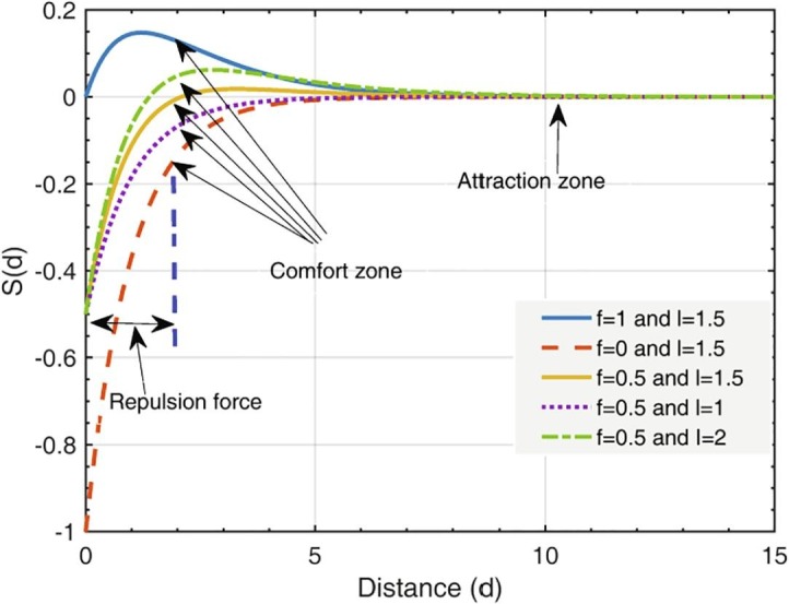
where $f$ denotes the intensity of attraction and $l$ denotes the attractive length scale. Fig. 6 illustrates the influence of the $s$-function on the social interaction of the grasshopper (repulsion and attraction). An interval of [0, 15] is considered for the distance $\left(d\right)$. It can be noticed that the repulsion force between the grasshoppers takes place at a distance between 0 and 2.079 units. After that, the grasshopper has entered its comfort zone, where there is no repulsion or attraction. The attraction of the grasshopper starts to increase after 2.079 until 4 and then further decreases gradually. A more clear demonstration is given in Fig. 7 , where different social behaviors can be observed in the artificial grasshoppers by altering values of $l$ and $f$. In this work, 0.5 and 1.5 are chosen as the values of $l$ and $f$ during the optimization process. The conceptual model of the repulsion force, comfort force, and the attraction force between the grasshoppers is given in Fig. 8 .

Fig. 6.

The behavior of the function $s$ with respect to the values of $f$ and $l$.

Fig. 7.

The performance of the $s$ function for various values of $f$ and $l$.

Fig. 8.

The embryonic illustration between individuals in a swarm of grasshoppers.

Eq. (24) can be updated by substituting $A_i$, $S_i,$ and $G_i$ components to solve the optimization problem. The mathematical model proposed by Mirjalili et al. [33] is thus given as follows:

$$X_i^d=C\left(\sum _{\begin{array}{c}j=1\\ j\ne i\end{array}}^{N}C\frac{{\mathit{ub}}_d-{\mathit{lb}}_d}{2}s\left(\left|X_j^d-X_i^d\right|\right)\frac{(x_j-x_i)}{d_{\mathit{ij}}}\right)+\widehat{T_d}$$ (29)

where ${\mathit{ub}}_d$ and ${\mathit{lb}}_d$ denote the upper and lower bounds respectively, in the $d^{\mathit{th}}$ dimension. $C$is a decreasing coefficient and is used to shrink the repulsion zone, comfort zone, and the attraction zone. $\widehat{T_d}$ denotes the target value in the $D^{\mathit{th}}$ dimension, and is also referred to as the best solution found. The $G_i$ component (gravity force) is ignored (i.e. considered to be zero) in Eq. (29) and $A_i$ (wind force) is always in the direction of the best solution $\widehat{T_d}$. The adaptive parameter $C$ was used twice to simulate the deceleration of the grasshoppers coming close to a source of food and eventually eating it. The first $C$ has been used to minimize the search region toward the target grasshopper as the iteration increases. The second $C$ is used to minimize the effect of repulsion, and attraction forces between grasshoppers proportional to the number iterations to shrink the attraction, repulsion, and comfort zones.

The value of the parameter $C$ is updated using Eq. (30). The mechanism balances between exploitation and exploration of the GOA and proportionally reduces the comfort zone to the number of iteration. $C_{\mathit{min}}$ and $C_{\mathit{max}}$ denote the minimum and maximum values of the adaptive parameter $C$, $t_{\mathit{max}}$ refers to the maximum number of iterations, and $t$ refers to the current iteration count.

$$C=C_{\mathit{max}}-t\frac{C_{\mathit{max}}-C_{\mathit{min}}}{t_{\mathit{max}}}$$ (30)

GOA is was applied and Action 1 to 5 were followed to solve the optimization problem of the grid-independent microgrid. All the steps of the proposed approach are clearly explained in Section 3.4.1 and Fig. 9 . At the commencement of the simulation, like any other population-based algorithm, GOA places some random particles in the search landscape. The particles move in the search landscape in accordance with the governing equations of the algorithm to solve the optimization problem. Recently, GOA has been applied to address various RE-based energy system problems, some of the recent works can be found in ref. [50], [51], [52], [53].

Fig. 9.

The flowchart of the overall REMS-GOA computational procedure.

3.4.1. Application of the GOA for optimal capacity planning problem

The computational steps of the devised GOA algorithm are as follows:

Step 1: Load input data.

• a)Load climatological database (ambient temperature, wind speed, solar irradiance).
• b)Load demand database.
• c)Load database of the economic indices and technical specifications of the microgrid components (according to Table 2).

Step 2: Initialization

• d)
  Set the GOA constants:

  • •
    Population size,$G=5$, Max iteration = 100, $C_{\mathit{min}}=0.1$, $C_{\mathit{max}}=0.9$, intensity of attraction $f=0.5$, $l=1.5$.
• e)
  Set constraint:

  • •
    REF (according to Eq. (22)) and DPSP (according to Eq. (23)).
• f)Set the search space:

The list of design variables is as follows. The dimension of the GOA algorithm is the number of design variables (according to Eq. (24)).

• •Lower bound and upper for $N_{\mathit{WT}}$ [0 1 0].
• •Lower bound and upper for $N_{\mathit{PV}}$ [0 4 5].
• •
  Lower bound and upper for $N_{\mathit{AD}}$ [0 3].

  • g)
    Randomly generate an initial swarm of $n$ grasshopper and apply to the objective function to evaluate the fitness of each candidate and determine the best one (T).
  • h)
    Update adaptive parameter $C$ using Eq. (30).

Step 3: Normalize distance between grasshoppers, update the position of the current search agent using Eq. (29).

• •Bring the current search agent back if it goes outside the boundaries of REF and DPSP.

Step 4: Update (T) if there is a better solution.

Step 5: Stopping criterion. If the number of iteration exceeds the maximum iterations then stop. The values of the control parameters used for the different algorithms and the overall flow chart of the proposed computational procedures are given in Table 5 and Fig. 9, respectively.

Table 5.

Optimization controlling parameters.

GOA	CSA	PSO
Population size (G): 5	Number of the nest: 5	Swarm size: 5
Number of iteration: 100	Number of iteration: 100	Max generation: 100
The parameter of shrinking factor: $\mathit{Cmin}=0.1$ and $\mathit{Cmax}=0.9$	Fractions of abandoned nests $P_a=0.2$	Inertia weight $w=1$
The intensity of attraction $f=0.5$ and $l=1.5$	Fractions of smart nests $P_c=0.5$	Acceleration coefficient: $C1=0.25$ and $C2=1.75$

4. Simulation results and discussion

This section centers on verifying the validity of the contributions introduced within the context of the developed optimal capacity planning method from different viewpoints and presents a cost-benefit analysis of the proposed microgrid based on the results obtained for the considered case study. The proposed microgrid presented in Fig. 2 (which can be considered to be a typical grid-independent microgrid for supplying electricity for remote residential housing) is employed to test and verify the effectiveness of the devised optimal planning capacity procedure. This is conducted by examining the impact of the contributions incorporated in the method compared to other approaches used in the planning studies of microgrid using numerical simulations. All simulations were performed using MATLAB software on an Intel Core i7-4770 CPU, 3.40 GHz PC.

4.1. Validation of the proposed rule-based energy management scheme

This section presents the results of the resiliency of the REMS before optimizing it using the proposed capacity planning algorithm (GOA). The simulation process is aimed at examining the resiliency of the REMS over a long period and to ascertain that the BT operating limit is not violated despite the occurrence of seasonal variation. In this context, the maximum allowable DOD of the BT is set at 70% and the initial SOC is set at 80%. The PV array was rated 5.8 kW; the BT bank was rated 45.2kW h each 12 V/250 Ah; the WT was rated 5 kW; and ${\mathrm{D}}_{\mathrm{g}\mathrm{e}\mathrm{n}}$ was rated 2 kW is used as an input for the REMS to examine the resiliency of the scheme and the rule-based algorithm used for implementing the scheme. Fig. 10 (a–c) depicts the few samples of the electricity mix of the various system components that composed the microgrid and its corresponding BT capacity at time step $t$ for the three seasonal variations (cold, hot and rainy season), whereas Fig. 10d depicts the results of the energy mix for a year. By referring to Fig. 10a, the rise, and fall of the $P_{\mathit{PV}}$ is reasonably smooth; this indicates that the irradiance is not disturbed by an abrupt change in the climatological conditions, such as a large cloud passing or rain. During the morning hours (0 h to 8 h), ${\mathit{POW}}^{\mathit{wt}}$ and ${\mathit{POW}}^{\mathit{pv}}$ are virtually zero; as such the BT discharges the energy stored in it to fulfil the energy demand (refer to the positive blue dotted line of Fig. 10a). As the sun starts to rise (8 h–9 h), PV and partially WT starts to generate electricity to fulfil the demand, and BT starts to charge (refer to the negative blue dotted lines of Fig. 10a). At the start of the sunset (15 h), BT, with the combined effort of WT and PV, starts to fulfil the demand. From there, BT and partially WT continue to supply the demand. Similarly, at 30 h, the BT has reached its minimum allowable limit to discharge (refer to Fig. 10a). Thus, the ${\mathrm{D}}_{\mathrm{g}\mathrm{e}\mathrm{n}}$ instantaneously switches ON to supply demand and starts to charge the BT. The ${\mathrm{D}}_{\mathrm{g}\mathrm{e}\mathrm{n}}$ is switched OFF immediately when the sun starts to rise. Fig. 10d illustrates the annual electricity mix under the operation of the proposed REMS. The aforementioned facts that have been demonstrated for 50 h during the cold, hot and rainy seasons can be noticed from the annual energy mix. Despite the continuous deviation in all the quantities, the REMS can able to manage and coordinate the power flow of the microgrid subsystems.

Fig. 10.

The electricity generation mix versus BT power, (a) the cold-season (b) the hot-season. The electricity generation mix versus BT power (c) the rainy-season (d) the simulation for one-year operation.

4.2. Verification of the outperformance grasshopper optimization algorithm on standard benchmark test functions

For validation of the proposed GOA, four popular standard benchmark functions comprising unimodal and multimodal functions (Schwefel, Goldstein, Michalewicz, and Sphere functions) were made used. The mathematical formulation of the functions, and their dimension and range are described in detail in Table 6 . The optimum solution found by GOA for test functions were compared with the ones found by PSO and CSA. PSO and CSA were applied to assess the performance of the GOA because of their vast usage in the field of equipment capacity planning of microgrids. The optimum values of the test function were run 30 times by the GOA, PSO, and CSA. Table 6 provides the results of the validation.

Table 6.

Standard benchmark test function.

Function name	Function type	Function	Dimension	Range	Optimum value
Schwefel’s	Multimodal	$f_1={\sum }_{i=1}^D-xsin\left(\left|\sqrt{x_i}\right|\right)$	2	[−500 500]	−837.9658
Goldstein	Multimodal	$f_2=[1+{\left(x_1+x_2+1\right)}^2\left(19-14x_1+3x_1^2-14x_2+6x_1{x}_2+3x_2^2\right)]\times [30+{(2x_1-3x_2)}^2(18-32x_1+12x_1^2+48x_2-36x_1{x}_2{+27x}_2^2]$	2	[−5 5]	3
Michalewicz	Multimodal	$f_3={\sum }_{i=1}^{D}sin\left(x_i\right){\left[sin\frac{{\mathit{ix}}_i^2}{\pi }\right]}^{20}$	2	[0 3.3]	−1.8013
Sphere	Unimodal	$f_2={\sum }_{i=1}^{D-1}{x}^2$	2	[−100 100]	1.84E−11

Regarding the solutions given in Table 7 , the quality of solutions found by the GOA yields better results in terms of nearing the optimal solution. For the $f_1$ function, the best solutions found by the GOA, PSO, and CSA are similar, but with slight differences in the mean. For $f_2,f_3$, and $f_4$, the GOA yields better results compare to its counterparts. Fig. 11, Fig. 12 present the shape of the test functions and their corresponding search history diagrams (convergence process) during the optimization process. It can be observed, that the multimodal test functions (refer to Fig. 11a, b, and 12a) has many local optimums, which make them worthy for benchmarking of a metaheuristic algorithm. The unimodal function (refer to Fig. 12b) has one global optimum with no local solutions. As per the search history diagram presented in Fig. 11, Fig. 12, the grasshoppers are inclined to the promising regions of the search landscape and eventually gather around the global optima (refer to the red dot in Fig. 11, Fig. 12). The pattern can be noticed in both multimodal and unimodal test functions. This result has demonstrated the capability of the GOA in balancing the exploitation and exploration to drive the grasshoppers near the global optima.

Table 7.

Comparison of solution quality.

Function	Function name	Algorithm	Best	Mean
$f_1$	Schwefel’s	PSO	−837.9658	−794.5384
		CSA	−837.6698	−837.6698
		GOA	−837.9658	−790.5904
$f_2$	Goldstein	PSO	3.0022	3.063153
		CSA	3.0008	3.017757
		GOA	3	3.001
$f_3$	Michalewicz	PSO	−1.8019	−1.8019
		CSA	−1.8016	−1.8016
		GOA	−1.8013	−1.8013
$f_4$	Sphere	PSO	3.72E−11	1.24E−06
		CSA	9.57E−08	4.65E−06
		GOA	1.84E−11	1.40E−10

Fig. 11.

Parameter space and search history diagram of the Schwefel’s and Goldstein function during the GOA optimization.

Fig. 12.

Parameter space and search history diagram of the Michalewicz and Sphere function during the GOA optimization.

4.3. Optimization of the hybrid grid-independent microgrid

The proposed optimization algorithm is aimed at determining the optimal capacity of the grid-independent microgrid meant to supply the demand of remote residential housing unit, at ${\mathit{DPSP}}_{\mathit{Desired}}$. In the literature, the DPSP value is interpreted to be valued from 0% to 1%. DPSP = 0% implies that the microgrid is autonomous full and has the provision of meeting an all-day demand without interruption.${\mathit{DPSP}}_{\mathit{Desired}}$ > 0 implies that the microgrid is autonomous basic, i.e. the microgrid cannot fulfil the demand for 24 h a day. The analysis in this section was performed for a DPSP value of 0%. To ensure the reliability of the proposed REMS-GOA in computing the optimal capacity of the grid-independent microgrid required to supply the demand, REMS-CSA and REMS-PSO are programmed and applied to the optimization problem. Accordingly, the values of the different controlling parameters used for the algorithms are given in Table 5.

The ideal convergence characteristic of the applied algorithms over 30 runs is depicted in Fig. 13 . The ordinate of the convergence curve represents the COE estimate and offers a platform for the comparison of the applied metaheuristic algorithms, whereas the abscissa represents the iteration count.

Fig. 13.

Convergence process of the applied algorithms.

At the start of the iteration process, the COE values are $0.3951/kW h, $0.3958/kW h, and $0.3857/kW h for REMS-GOA, REMS-CSA, and REMS-PSO, respectively. Afterward, the values decrease for all the applied algorithms during the iteration process. This means that the algorithms minimize the COE by moving towards the promising regions of the search landscape and eventually stop when the maximum iteration is reached. Consequently, a decrease in the objective function is vital because it leads to having extra information about the optimal values of the design variables. A thorough examination of the convergence curve indicates that REMS-GOA yields a better result as it offers the minimum objective function of $0.3656/kW h, followed by REMS-CSA with $0.3662/kW h and REMS-PSO with $0.3674/kW h. Nevertheless, the REMS-GOA convergence period in the minimum condition is 17 s and better than the REMS-CSA, which is 25 s. The REMS-PSO converges to the minimum condition at 7 s because PSO is prone to premature convergences [11]. Full details of the results obtained for the considered microgrid in the case of${\mathit{DPSP}}_{\mathit{Desired}}$ = 0% are presented in Table 8 . The minimum COE, which is regarded as the best choice, is $0.3656/kW h, as determined by employing the REMS-GOA method. Ranked second is convergence found by REMS-CSA, and Rank third is the one found by REMS-PSO. Thus, it can be concluded that the proposed REMS-GOA offers better performance in all aspects and can successfully be used to find the optimal solution of a complex microgrid design problem compared to its counterparts. The optimal system configuration found consists of a 7150 W capacity of PV array, 4000 W WT, 4.52 kW h BT bank capacity and ${\mathrm{D}}_{\mathrm{g}\mathrm{e}\mathrm{n}}$ rated at 5 kW. For the optimal configuration achieved, we show the plot of the annual PV and WT output power in Fig. 14, Fig. 15 , respectively. Fig. 16 depicts the annual electricity mix, zoomed version of the electricity mix (at the top left), and the annual SOC of the BT (at the top right). The zoomed version of the SOC for the three different seasons is presented in Fig. 17 . One can notice in Fig. 17b that BT bank is exploited more intensively and is more vulnerable during the hot season, compared to the cloudy and rainy season, this is because of the high demand for energy during the season.

Table 8.

Optimal results obtained for the grid-independent microgrid for ${\mathit{DPSP}}_{\mathit{Desired}}=0\%$.

	REMS-GOA	REMS-CSA	REMS-PSO
${\mathit{DPSP}}_{\mathit{Desired}}$	0	0	0
AD (The larger the number, the better the system)	3	3	2
Number of PV panel	26	29	30
Number of WT	4	6	7
${\mathrm{D}}_{\mathrm{g}\mathrm{e}\mathrm{n}}$ capacity (kW)	5	5	5
BSS capacity (kW h)	45.2	45.2	45.2
COE ($/kW h)	0.3656	0.3662	0.3674
System capital cost ($)	47,572.5	55,346.25	58,937.5

Fig. 14.

The power generated by PV array.

Fig. 15.

The power generated by the WT.

Fig. 16.

Electricity generation mix for optimal system (bottom), zoomed-in version (top left) and its SOC (top right).

Fig. 17.

Zoomed view of the SOC in Fig. 16 for the different seasonal.

4.3.1. Simultaneous minimization of the objective functions

In the previous section (Section 4.3) the two objective functions, COE and DPSP were aggregated into one single objective to achieved DPSP = 0%. The optimization problem then becomes a mono-objective optimization problem. In other words, the COE becomes the main objective; while DPSP changed to a constraint. Hence, the approach has the disadvantage of determining only one single optimal solution (the best system configuration at a ${\mathit{DPSP}}_{\mathit{Desired}}$ level) that does not represent a trade-off between multiple objective functions. In this light, the current study further exploits the capability of a maiden multi-objective grasshopper optimization algorithm (MOGOA) embedded with Pareto optimal front to optimize the microgrid. MOGOA can simultaneously and independently optimize the objective functions (COE and DPSP), and perhaps the impact of the variation of the DPSP can only be realized by simultaneously considering both objectives. The multi-objective optimization problem (MOOP) is performed by linearly combining two objectives. To illustrate this fact comparatively, the problem is expressed as follows.

$$\mathrm{M}\mathrm{i}\mathrm{n}\mathrm{i}\mathrm{m}\mathrm{i}\mathrm{z}\mathrm{e}w{F}_1+\left(1-w\right)\phi .PF.F_2$$ (32)

The equation has been applied to the two conflicting objectives, $F_1=COE$ and $F_2=DPSP$. $w$ in Eq. (32) denote a weighting factor randomly generated in the range of (0, 1). Its value is set at zero and progressively increased in the step of 0.05 up to 1. $\phi$ is a scaling factor chosen as 1000. The two objectives have different units in the MOOP, a penalty factor ($\mathit{PF})$ is considered to properly balance the objectives.

Two scenarios, case #1 and case #2 each corresponds to 5, and 10 residential housing units are considered to demonstrate the approach. MOGOA is run for 100 iterations and the solutions obtained for the microgrid configurations offer a remarkable and consistent distribution in the non-dominated front (refer to Fig. 18, Fig. 19 ). The results obtained not only offer the optimum solution, but a set of optimum trade-off solutions (non-dominated solutions) in a Pareto front thereby giving the decision-makers several options to choose from. The Pareto-optimal front of the microgrid configuration for case #1 and case #2 is shown in Fig. 18, Fig. 19. For case #1, 20 selected solutions from the Pareto-front are extracted along with some vital information which is shown in Table 9 .

Fig. 18.

2D Pareto front of microgrid system configuration considering COE and DPSP for case #1.

Fig. 19.

2D Pareto front of microgrid system configuration considering COE and DPSP for case #2.

Table 9.

20 selected sets of non-dominated solutions from the Pareto front of case #1.

	PV (Units)	WT (Units)	AD (Days)	COE ($/kW h)	DPSP (%)	REF (%)
Solution # 1	19.8	6.0	3.0	0.255	0.271	90.50
Solution # 2	19.2	6.0	3.0	0.254	0.273	90.36
Solution # 3	18.4	6.0	3.0	0.252	0.279	90.17
Solution # 4	18.2	6.0	3.0	0.252	0.280	90.11
Solution # 5	18.1	6.0	3.0	0.252	0.281	90.06
Solution # 6	17.9	6.0	3.0	0.251	0.282	90.02
Solution # 7	17.1	6.0	3.0	0.250	0.285	89.78
Solution # 8	16.9	6.0	3.0	0.250	0.286	89.74
Solution # 9	16.4	6.0	2.9	0.249	0.288	89.59
Solution # 10	16.1	6.0	2.8	0.248	0.290	89.52
Solution # 11	15.5	6.0	2.8	0.247	0.292	89.33
Solution # 12	15.0	6.0	2.8	0.246	0.293	89.22
Solution # 13	14.3	6.0	2.5	0.245	0.295	89.03
Solution # 14	14.0	6.0	2.5	0.244	0.294	88.95
Solution # 15	13.6	6.0	2.3	0.244	0.295	88.83
Solution # 16	12.5	6.0	2.3	0.242	0.298	88.60
Solution # 17	12.0	6.0	2.3	0.241	0.301	88.52
Solution # 18	11.6	6.0	2.3	0.240	0.303	88.50
Solution # 19	11.1	6.0	2.3	0.239	0.305	88.48
Solution # 20	10.3	6.0	2.3	0.238	0.311	88.43

Using the above technique, multiple sets of Pareto optimal solutions for the grid-independent microgrid system are obtained. For example, if solution #1 of case #1 is chosen by the decision-maker, the microgrid will constitute 6 WTs, an approximate of 20 units of PV modules, 3 days of system autonomy, etc., and the solution corresponds to REF of 90.50%, DPSP of 0.271%, and COE of $0.255/kW h.

4.4. Analysis based on CO₂ Emission, fuel Consumption, and COE

Based on the capacity of the microgrid computed using the proposed REMS-GOA for ${\mathit{DPSP}}_{\mathit{Desired}}=0\%$ (refer to Section 4.3), an overall comparison between the proposed grid-independent microgrid operating under control of the REMS and a conventional ${\mathrm{D}}_{\mathrm{g}\mathrm{e}\mathrm{n}}$ system is made; because the residential housing units presently depend solely on conventional ${\mathrm{D}}_{\mathrm{g}\mathrm{e}\mathrm{n}}$ system. The comparison is made in terms of CO₂ emission, $\mathit{FC},$and $\mathit{COE}$. Fig. 20a illustrates the ON/OFF operation of ${\mathrm{D}}_{\mathrm{g}\mathrm{e}\mathrm{n}}$ under the control of the RfEMS (scenario 1) versus that of the conventional ${\mathrm{D}}_{\mathrm{g}\mathrm{e}\mathrm{n}}$ considered as the reference for comparison of power supply for the remote residences (scenario 2). By using the IPCC method discussed in Section 2.1.4 [44], the two scenarios can be examined in terms of CO₂ avoidance, $\mathit{COE}$ and$\mathit{FC}$. The results of the comparison of the two scenarios is illustrated in Fig. 21 . The analysis reveals that the proposed microgrid has significantly reduced $\mathit{FC}$ and ${\mathit{CO}}_2$ emission produced by the conventional ${\mathrm{D}}_{\mathrm{g}\mathrm{e}\mathrm{n}}$ by 92.4% and 92.3% respectively. Additionally, the $\mathit{COE}$ was reduced by 79.8%. Hence, it can be concluded that the proposed microgrid operating under the control of the REMS has a less environmental impact as compared to the conventional ${\mathrm{D}}_{\mathrm{g}\mathrm{e}\mathrm{n}}$ power plant taken as a reference. For further examination, it can be observed that the ON/OFF of the ${\mathrm{D}}_{\mathrm{g}\mathrm{e}\mathrm{n}}$ is well balanced with the SOC of the BT bank (Fig. 20b). As seen in Fig. 20a the ${\mathrm{D}}_{\mathrm{g}\mathrm{e}\mathrm{n}}$ operates for a longer period during the hot season, this effect can be observed in Fig. 20b, as the SOC of the BT bank, virtually becomes 100% as compared to that in the rainy and cold seasons. For this reason, the ${\mathrm{D}}_{\mathrm{g}\mathrm{e}\mathrm{n}}$ is turned on for many hours during the hot season to compensate for the demand when the BT bank is depleted or when it reaches its minimum allowable SOC.

Fig. 20a.

ON/OFF operation of ${\mathrm{D}}_{\mathrm{g}\mathrm{e}\mathrm{n}}$ under the control proposed REMS versus the usage ${\mathrm{D}}_{\mathrm{g}\mathrm{e}\mathrm{n}}$.

Fig. 21.

The comparison of scenario 1 and 2 in terms of the annual FC, CO2 emission and the COE.

Fig. 20b.

The SOC of the BT under the control proposed REMS versus the usage ${\mathrm{D}}_{\mathrm{g}\mathrm{e}\mathrm{n}}.$

4.5. Energy balance analysis

The amount of energy flow based on running the program simulating the REMS of the microgrid using the optimum capacities of its component obtained by the proposed optimal capacity planning approach is shown in Fig. 22 . Fig. 22(a and b) illustrate the total and percentage contribution of power produced by the energy sources in the microgrid during the cold, hot, and rainy seasons, respectively. Such analysis can be applied to other operational horizons (for example, for the whole project’s life span) by simply changing and adapting the input parameters to the model. One other point that should not be ignored is the size of the microgrid element computed using the proposed optimal capacity approach for the same operational project lifespan when performing such an analysis. This mechanism will avert the occurrence of discrepancies between the demand and supply within the microgrid. As demonstrated in Fig. 22b, a total of 44% of the energy generated by the microgrid comes from the PV array, and 26% is from the WT. ${\mathrm{D}}_{\mathrm{g}\mathrm{e}\mathrm{n}}$ and BT contributed 14% and 16%, respectively.

Fig. 22.

(a) The annual power generated by the main energy generators in the different season (b) the percentage contribution of electricity generation by the system component.

A study was also conducted regarding the excess power produced by the microgrid. In this light, Fig. 23 a portrays the plot of the annual excess power produced in each season against the energy demand, and Fig. 23b illustrates the percentage of excess power generated in each season. The results indicate that a total of 981.4 kW excess power would be produced annually, of which approximately 811.3 kW, 12.5 kW, and 171.5 kW would be produced during cold, hot, and rainy seasons respectively. One can note that virtually no amount of excess electricity is produced during the hot season (refer to Fig. 23a and b), this is because of the high demand for energy during the hot season. Similarly, BT is extremely utilized during the hot season as shown, as illustrated previously in Fig. 20b; therefore, it is an indication that a smaller amount of excess electricity will be produced during the hot season because BT is not allowed to fully charged during the hot season.

Fig. 23.

(a) The annual excess power produced versus energy demand (b) the seasonal percentage of excess power produced.

4.6. Analysis of the breakdown of the microgrid subsystem procurement cost

A breakdown of the microgrid subsystem procurement cost for the best combination of the capacities of its sub-system’s element computed using the devised method, which implements the REMS and optimizes by GOA for the considered case study, is given in Fig. 24 . The contribution of the procurement cost for the WT accounts for approximately 25.3% of the total procurement cost of the microgrid, the PV array accounts for nearly 32.6%, and the converters account approximately 10%, followed by the BT, which contributes up to 24.2%. Remarkably, unlike other grid-independent microgrids, in which the cost of the BT bank is leading [54], the BT comes third among the microgrid elements in terms of the initial cost in this project. This is due to the extremely complementary time behavior of the wind and solar resources in the study region. Moreover, the COE computed for the considered microgrid is found to be $0.36563/kW h assuming the proposed microgrid is to fully supply the residential energy demand. One can notice that the electricity price is much lower compared to the usage of standalone ${\mathrm{D}}_{\mathrm{g}\mathrm{e}\mathrm{n}}$, as the COE is found to be $1.81/kW h. Therefore, the calculated COE in this project is competitive to conventional ${\mathrm{D}}_{\mathrm{g}\mathrm{e}\mathrm{n}}$ use by most off-grid communities. This makes the project economically viable for installation in Damaturu, Yobe State, Nigeria, since the required energy demand is currently being supplied by conventional ${\mathrm{D}}_{\mathrm{g}\mathrm{e}\mathrm{n}}$. It is expected that the deployment of the project will improve the reliability of power supply in the case study region, reduce GHG, and effectively contribute to the region's sustainable development goals.

Fig. 24.

The breakdown of the optimal system cost computed using GOA.

4.7. Sensitivity analysis report

This section presents the result of a sensitivity analysis implemented on the grid-independent microgrid. The sensitivity analysis was performed to examine the performance of the microgrid due to uncertainties on the system inputs that may arise in the future. Regarding the analysis, the influence of climatological conditions (wind speed, solar radiation, and temperature), diesel price, BT bank capacity, and SOC set-point is considered in this study. The parameters were carefully chosen based on the following motives:

• •The effect of climatological conditions is taken into account to model a worse day scenario (a windy or cloudy sky condition).
• •The price of crude oil has in recent times witnessed a substantial and unprecedented decline due to the COVID-19 pandemic, and it is expected to further decrease soon owing to the advent of the electric vehicle and 5G technologies.
• •BT storage systems are the most vulnerable and the most expensive component in the microgrid, probably with less lifespan.

4.7.1. Effect of SOC Set-Point, PV power Output, diesel Price, and WT power output

The result obtained for the optimal system configuration for the${\mathit{DPSP}}_{\mathit{Desired}}$ = 0% is chosen to demonstrate the impact of uncertain changes on PV power output, diesel price, WT power output, and SOC set-point, details of the result is given in Table 8. The sensitivity adjustment was made on a 10% increment/decrement. In this light, the sensitivity curves obtained due to the aforementioned uncertainties is presented in Fig. 25 . The “Base” point on the abscissa refers to the nominal values of the sensitivity adjustment (without increment or decrement). It can be observed that the diesel price has a tremendous effect on COE. As diesel prices increases, COE also increases. On the contrary, the COE value becomes lower for a higher value of PV and WT power and vice versa. This is because the ${\mathrm{D}}_{\mathrm{g}\mathrm{e}\mathrm{n}}$ will operate less when the PV and WT generate more power. Equally, an increase in the SOC set-point will cause a decrease in COE, but to the disadvantage of the BT bank. Finally, one can observe that at the base point, COE achieved is equal to the one computed by the GOA, i.e. $0.3656/kW h (refer to Table 8, Section 4.3).

Fig. 25.

Sensitivity analysis: effect of diesel price, PV power, WT power, and SOC set-point on the COE and DPSP.

4.7.2. Effect of the battery bank capacity

Solution #1 of case #1 with COE of $0.255 kW h and DPSP of 0.271% (refer to Table 9) is chosen as a reference to demonstrate the effect of changes on BT bank capacity. The sensitivity adjustment for the BT bank capacity was made from −50% to 150%. The sensitivity curves obtained are depicted in Fig. 26 . The “Base” point on the abscissa refers to the initial nominal BT capacity (45.2 kW h) chosen for the design. The right and left ordinates depict the DPSP and COE values for different BT capacities. Based on the curves, it can be observed that an increase in the level of BT capacity will reduce the DPSP and lead to an increment in the COE. Any decrease in the BT capacity will lower the COE, although to the detriment of DPSP. This analysis is important because it helps the designer to select the capacity of a BT bank based on the level of individual requirements.

Fig. 26.

Sensitivity analysis: Effect of BT bank capacity on the COE and DPSP.

5. Conclusions and future work

This study considered a conceptual grid-independent microgrid to confirm the validity of the proposed EMS and optimal capacity planning method. The microgrid is meant to meet the energy demand of the residential housing unit in a remote community situated in Yobe State, Nigeria. The RE sources in the proposed microgrid can be updated depending on the RE potential of other regions. Accordingly, the PV and WT were considered as the main energy sources in the microgrid. The selection of the RE generation system, whose optimum sizes are under question, is context-dependent and requires prior viability studies to be conducted on the potentials for the utilization in the target area of the study. To put it differently, the devised method in this work is not principally targeted on and reserved for residential load only. The method can be practically applied to other energy projects with different load profiles (such as agricultural loads, industrial loads, and commercial loads), by simply modifying the corresponding variables and following the same approach.

Since the results of this work support the idea that implementing a proper EMS program while optimally sizing the elements of microgrid leads to the reduction of the overall system cost according to the reduced sizes of some of the elements. Therefore, REMS has been introduced to prioritize the utilization RE first and coordinate the power flow of the microgrid components whilst attempting to highlight the effectiveness of the GOA in solving for the considered problem. The numerical simulation results obtained have demonstrated the efficacy of the abovementioned advanced, cutting-edge approaches in contributing toward minimizing the cost of the grid-independent microgrid and the computational complexity of the problem-solving. Furthermore, since the optimal capacity planning problems of microgrids are nonlinear and non-convex combinational optimization problems, to make it amenable to other mathematical optimization methods, the performance of the proposed REM-GOA method is evaluated through a comparative study with REM-PSO and REMS-CSA in terms optimality of the solution and its convergence when applied to the optimal equipment capacity planning of a conceptualized microgrid for the considered case region. The present study shown has demonstrated that REM-GOA yields a better result as it offers the minimum objective function of $0.3656/kW h, compared to REMS-CSA and REMS-PSO which yields a COE of $0.3662/kW h and $0.3674/kW h respectively at ${\mathit{DPSP}}_{\mathit{Desired}}=0\%$. The simulation results have also indicated that the proposed can REMS has significantly reduced the ${\mathit{CO}}_2$emission, $\mathit{FC},$ and COE by 92.3%, 92.4%, and 79.8%, respectively.

To make the proposed microgrid smarter, it is recommended that future work should focus on the following key areas. The first is to develop a more sophisticated EMS considering microgrid pool (the interconnection of two or more microgrids) and incorporate it with the proposed optimal capacity method. The second key area is to focus on providing a platform for the consideration of harmonics originating from power conversion devices and nonlinear loads while designing the microgrid. The third area is to address the uncertainties inherent to various inputs variables (e.g., system losses, the inflation rate, and energy demand growth) of the microgrid network using uncertainty analysis methods, such as robust programming, chance-constrained, and Monte Carlo simulations. Moreover, the present study considered a single storage system. Future work can consider the integration of hydrogen storage, in which an EL can be used to produce H₂. Modern equipment and other household appliances use dc voltage for their operation. Researchers have also discovered the benefit of a dc microgrid for localized load and the notion is to rewire homes to run on dc. Therefore, it is worthwhile to further explore the economic and technical viability of a dc microgrid. Algorithms like chaotic ant swarm [55], memetic algorithm [56], cultural Algorithm [57], salp swarm optimization [58], along with other nature-inspired approaches used in various optimization studies, are also likely to enrich the future research in RE-based energy system optimization studies.

CRediT authorship contribution statement

Abba Lawan Bukar: Conceptualization, Methodology, Software, Validation, Investigation, Formal analysis, Writing - original draft, Writing - review & editing, Funding acquisition. Chee Wei Tan: Conceptualization, Writing - review & editing, Visualization, Supervision, Funding acquisition. Lau Kwan Yiew: Data curation, Investigation, Visualization, Project administration, Supervision. Razman Ayop: Data curation, Formal analysis, Visualization, Writing - review & editing. Wen-Shan Tan: Writing - review & editing.

Declaration of Competing Interest

The authors declare that they have no known competing financial interests or personal relationships that could have appeared to influence the work reported in this paper.

References

- 1.Zhang W., Maleki A., Rosen M.A. A heuristic-based approach for optimizing a small independent solar and wind hybrid power scheme incorporating load forecasting. J Cleaner Prod. 2019;241 [Google Scholar]
- 2.Maleki A., Nazari M.A., Pourfayaz F. Harmony search optimization for optimum sizing of hybrid solar schemes based on battery storage unit. Energy Rep. 2020 [Google Scholar]
- 3.Bukar A.L., Modu B., Gwoma Z.M., Mustapha M., Buji A.B., Lawan M.B. Economic assessment of a pv/diesel/battery hybrid energy system for a non-electrified remote village in Nigeria. Eur J Eng Res Sci. 2017;2:21–31. [Google Scholar]
- 4.Modu B., Aliyu A., Bukar A., Abdulkadir M., Gwoma Z., Mustapha M. Techno-economic analysis of off-grid hybrid pv-diesel-battery system in Katsina State, Nigeria. Arid Zone J Eng Technol Environ. 2018;14:317. [Google Scholar]
- 5.Bukar AL, Tan CW, Lau KY, Marwanto A. Economic analysis of residential grid-connected photovoltaic system with lithium-ion battery storage. In 2019 IEEE conference on energy conversion (CENCON): IEEE; 2019. p. 153–8.
- 6.Mohseni S., Brent A.C., Burmester D. A demand response-centred approach to the long-term equipment capacity planning of grid-independent micro-grids optimized by the moth-flame optimization algorithm. Energy Convers Manage. 2019;200 [Google Scholar]
- 7.García-Olivares A., Solé J., Osychenko O. Transportation in a 100% renewable energy system. Energy Convers Manage. 2018;158:266–285. [Google Scholar]
- 8.Nazari M.A., Aslani A., Ghasempour R. Analysis of solar farm site selection based on TOPSIS approach. Int J Social Ecol Sustainable Dev (IJSESD) 2018;9:12–25. [Google Scholar]
- 9.Dehghani Madvar M., Alhuyi Nazari M., Tabe Arjmand J., Aslani A., Ghasempour R., Ahmadi M.H. Analysis of stakeholder roles and the challenges of solar energy utilization in Iran. Int J Low-Carbon Technol. 2018;13:438–451. [Google Scholar]
- 10.Ogbonnaya C., Turan A., Abeykoon C. Energy and exergy efficiencies enhancement analysis of integrated photovoltaic-based energy systems. J Storage Mater. 2019;26 [Google Scholar]
- 11.Mohseni S., Brent A.C. Economic viability assessment of sustainable hydrogen production, storage, and utilization technologies integrated into on-and off-grid micro-grids: a performance comparison of different meta-heuristics. Int J Hydrogen Energy. 2019 [Google Scholar]
- 12.Ongsakul W., Dieu V.N. Crc Press; 2016. Artificial intelligence in power system optimization. [Google Scholar]
- 13.Hakimi S., Tafreshi S.M., Kashefi A. (PSO). 2007 IEEE international conference on automation and logistics: IEEE. 2007. Unit sizing of a stand-alone hybrid power system using particle swarm optimization; pp. 3107–3112. [Google Scholar]
- 14.Chris M., Giri V., Michael S., Afzal S., Ryan F., Bala C. Optimal technology selection and operation of commercial-building microgrids. IEEE Trans Power Syst. 2008;23:975–982. [Google Scholar]
- 15.Brunetto C., Tina G. Optimal hydrogen storage sizing for wind power plants in day ahead electricity market. IET Renew Power Gener. 2007;1:220–226. [Google Scholar]
- 16.Sadeghzadeh S, Ansarian M. Distributed generation and renewable planning with a linear programming model. In 2006 IEEE international power and energy conference: IEEE; 2006. p. 48–53.
- 17.Hernandez-Aramburo C.A., Green T.C., Mugniot N. Fuel consumption minimization of a microgrid. IEEE Trans Ind Appl. 2005;41:673–681. [Google Scholar]
- 18.Lo C.H., Anderson M.D. Economic dispatch and optimal sizing of battery energy storage systems in utility load-leveling operations. IEEE Trans Energy Convers. 1999;14:824–829. [Google Scholar]
- 19.Lorestani A., Gharehpetian G., Nazari M.H. Optimal sizing and techno-economic analysis of energy-and cost-efficient standalone multi-carrier microgrid. Energy. 2019;178:751–764. [Google Scholar]
- 20.Zhang W., Maleki A., Rosen M.A., Liu J. Sizing a stand-alone solar-wind-hydrogen energy system using weather forecasting and a hybrid search optimization algorithm. Energy Convers Manage. 2019;180:609–621. [Google Scholar]
- 21.Dong W., Li Y., Xiang J. Optimal sizing of a stand-alone hybrid power system based on battery/hydrogen with an improved ant colony optimization. Energies. 2016;9:785. [Google Scholar]
- 22.Kaabeche A., Diaf S., Ibtiouen R. Firefly-inspired algorithm for optimal sizing of the renewable hybrid system considering reliability criteria. Sol Energy. 2017;155:727–738. [Google Scholar]
- 23.Shang C., Srinivasan D., Reindl T. An improved particle swarm optimization algorithm applied to battery sizing for stand-alone hybrid power systems. Int J Electr Power Energy Syst. 2016;74:104–117. [Google Scholar]
- 24.Zolfaghari M., Ghaffarzadeh N., Ardakani A.J. Optimal sizing of battery energy storage systems in off-grid microgrids using convex optimization. J Storage Mater. 2019;23:44–56. [Google Scholar]
- 25.Nagapurkar P., Smith J.D. Techno-economic optimization and environmental Life Cycle Assessment (LCA) of microgrids located in the US using genetic algorithm. Energy Convers Manage. 2019;181:272–291. [Google Scholar]
- 26.Singh S., Singh M., Kaushik S.C. Feasibility study of an islanded microgrid in rural area consisting of PV, wind, biomass and battery energy storage system. Energy Convers Manage. 2016;128:178–190. [Google Scholar]
- 27.Maleki A., Pourfayaz F. Sizing of stand-alone photovoltaic/wind/diesel system with battery and fuel cell storage devices by harmony search algorithm. J Storage Mater. 2015;2:30–42. [Google Scholar]
- 28.Sharma S., Bhattacharjee S., Bhattacharya A. Grey wolf optimisation for optimal sizing of battery energy storage device to minimise operation cost of microgrid. IET Gener Transm Distrib. 2016;10:625–637. [Google Scholar]
- 29.Fetanat A., Khorasaninejad E. Size optimization for hybrid photovoltaic–wind energy system using ant colony optimization for continuous domains based integer programming. Appl Soft Comput. 2015;31:196–209. [Google Scholar]
- 30.Ghorbani N., Kasaeian A., Toopshekan A., Bahrami L., Maghami A. Optimizing a hybrid wind-PV-battery system using GA-PSO and MOPSO for reducing cost and increasing reliability. Energy. 2018;154:581–591. [Google Scholar]
- 31.Yang X-S. A new metaheuristic bat-inspired algorithm. Nature inspired cooperative strategies for optimization (NICSO 2010): Springer; 2010. p. 65–74.
- 32.Saremi S., Mirjalili S., Lewis A. Grasshopper optimisation algorithm: theory and application. Adv Eng Softw. 2017;105:30–47. [Google Scholar]
- 33.Mirjalili S.Z., Mirjalili S., Saremi S., Faris H., Aljarah I. Grasshopper optimization algorithm for multi-objective optimization problems. Appl Intell. 2018;48:805–820. [Google Scholar]
- 34.Seifi A., Moradi M.H., Abedini M., Jahangiri A. An optimal programming among renewable energy resources and storage devices for responsive load integration in residential applications using hybrid of grey wolf and shark smell algorithms. J Storage Mater. 2020;27 [Google Scholar]
- 35.Maleki A., Pourfayaz F. Optimal sizing of autonomous hybrid photovoltaic/wind/battery power system with LPSP technology by using evolutionary algorithms. Sol Energy. 2015;115:471–483. [Google Scholar]
- 36.Lan H., Wen S., Hong Y.-Y., David C.Y., Zhang L. Optimal sizing of hybrid PV/diesel/battery in ship power system. Appl Energy. 2015;158:26–34. [Google Scholar]
- 37.Suntech, Direct industry. https://pdf.directindustry.com/pdf/suntech-power-corporation/stp275s-stp270s-20-wem/54793-588789.html [accessed 04.18.2017].
- 38.Central Bank of Nigeria (CBN). current interest rate. https://www.cbn.gov.ng/ [accessed 08.10.2019].
- 39.Ogunjuyigbe A.S.O., Ayodele T.R., Akinola O.A. Optimal allocation and sizing of PV/Wind/Split-diesel/Battery hybrid energy system for minimizing life cycle cost, carbon emission and dump energy of remote residential building. Appl Energy. 2016;171:153–171. [Google Scholar]
- 40.Zhang L, Barakat G, Yassine A. Design and optimal sizing of hybrid PV/wind/diesel system with battery storage by using DIRECT search algorithm. In 2012 15th international power electronics and motion control conference (EPE/PEMC): IEEE; 2012. p. DS3b. 19-1-DS3b. -7.
- 41.Ayodele T., Ogunjuyigbe A. Increasing household solar energy penetration through load partitioning based on quality of life: the case study of Nigeria. Sustainable Cities Soc. 2015;18:21–31. [Google Scholar]
- 42.Yahiaoui A., Fodhil F., Benmansour K., Tadjine M., Cheggaga N. Grey wolf optimizer for optimal design of hybrid renewable energy system PV-diesel Generator-battery: application to the case of Djanet city of Algeria. Sol Energy. 2017;158:941–951. [Google Scholar]
- 43.Dufo-López R., Bernal-Agustín J.L. Multi-objective design of PV–wind–diesel–hydrogen–battery systems. Renewable Energy. 2008;33:2559–2572. [Google Scholar]
- 44.Cozzolino R., Tribioli L., Bella G. Power management of a hybrid renewable system for artificial islands: a case study. Energy. 2016;106:774–789. [Google Scholar]
- 45.Bukar A.L., Tan C.W. A review on stand-alone photovoltaic-wind energy system with fuel cell: system optimization and energy management strategy. J Cleaner Prod. 2019 [Google Scholar]
- 46.Bhatti A.R., Salam Z. A rule-based energy management scheme for uninterrupted electric vehicles charging at constant price using photovoltaic-grid system. Renewable Energy. 2018;125:384–400. [Google Scholar]
- 47.Nigerian Meteorological Agency (NIMET). https://nimet.gov.ng/nwp Retrieved [accessed 04.18.2017].
- 48.Zhu B., Tazvinga H., Xia X. Switched model predictive control for energy dispatching of a photovoltaic-diesel-battery hybrid power system. IEEE Trans Control Syst Technol. 2014;23:1229–1236. [Google Scholar]
- 49.Maleki A., Pourfayaz F., Hafeznia H., Rosen M.A. A novel framework for optimal photovoltaic size and location in remote areas using a hybrid method: a case study of eastern Iran. Energy Convers Manage. 2017;153:129–143. [Google Scholar]
- 50.Barman M., Choudhury N.D., Sutradhar S. A regional hybrid GOA-SVM model based on similar day approach for short-term load forecasting in Assam, India. Energy. 2018;145:710–720. [Google Scholar]
- 51.Jumani T.A., Mustafa M.W., Md Rasid M., Mirjat N.H., Leghari Z.H., Saeed M.S. Optimal voltage and frequency control of an islanded microgrid using grasshopper optimization algorithm. Energies. 2018;11:3191. [Google Scholar]
- 52.Sultana U., Khairuddin A.B., Sultana B., Rasheed N., Qazi S.H., Malik N.R. Placement and sizing of multiple distributed generation and battery swapping stations using grasshopper optimizer algorithm. Energy. 2018;165:408–421. [Google Scholar]
- 53.Gampa S.R., Jasthi K., Goli P., Das D., Bansal R. Grasshopper optimization algorithm based two stage fuzzy multiobjective approach for optimum sizing and placement of distributed generations, shunt capacitors and electric vehicle charging stations. J Storage Mater. 2020;27 [Google Scholar]
- 54.Ma T., Yang H., Lu L. A feasibility study of a stand-alone hybrid solar–wind–battery system for a remote island. Appl Energy. 2014;121:149–158. [Google Scholar]
- 55.Zhang C., Cui G., Peng F. A novel hybrid chaotic ant swarm algorithm for heat exchanger networks synthesis. Appl Therm Eng. 2016;104:707–719. [Google Scholar]
- 56.Brownlee J. Clever algorithms: nature-inspired programming recipes. Jason Brownlee; 2011.
- 57.Sinha S., Chandel S.S. Review of recent trends in optimization techniques for solar photovoltaic–wind based hybrid energy systems. Renew Sustainable Energy Rev. 2015;50:755–769. [Google Scholar]
- 58.Mirjalili S., Gandomi A.H., Mirjalili S.Z., Saremi S., Faris H., Mirjalili S.M. Salp Swarm Algorithm: a bio-inspired optimizer for engineering design problems. Adv Eng Softw. 2017;114:163–191. [Google Scholar]