Toward Harmonizing Ecotoxicity Characterization in Life Cycle Impact Assessment

Abstract

Ecosystem quality is an important area of protection in life cycle impact assessment (LCIA). Chemical pollution has adverse impacts on ecosystems on a global scale. To improve methods for assessing ecosystem impacts, the Life Cycle Initiative hosted by the United Nations Environment Programme established a task force to evaluate the state‐of‐the‐science in modeling chemical exposure of organisms and the resulting ecotoxicological effects for use in LCIA. The outcome of the task force work will be global guidance and harmonization by recommending changes to the existing practice of exposure and effect modeling in ecotoxicity characterization. These changes will reflect the current science and ensure the stability of recommended practice. Recommendations must work within the needs of LCIA in terms of 1) operating on information from any inventory reporting chemical emissions with limited spatiotemporal information, 2) applying best estimates rather than conservative assumptions to ensure unbiased comparison with results for other impact categories, and 3) yielding results that are additive across substances and life cycle stages and that will allow a quantitative expression of damage to the exposed ecosystem. We describe the current framework and discuss research questions identified in a roadmap. Primary research questions relate to the approach toward ecotoxicological effect assessment, the need to clarify the method’s scope and interpretation of its results, the need to consider additional environmental compartments and impact pathways, and the relevance of effect metrics other than the currently applied geometric mean of toxicity effect data across species. Because they often dominate ecotoxicity results in LCIA, we give metals a special focus, including consideration of their possible essentiality and changes in environmental bioavailability. We conclude with a summary of key questions along with preliminary recommendations to address them as well as open questions that require additional research efforts.

INTRODUCTION

As part of an ongoing effort to improve ecotoxicity characterization in life cycle impact assessment (LCIA), the goal of the present review is to present and discuss existing research and research challenges, and then provide a path forward, building on earlier consensus‐building efforts.

Addressing ecotoxicity

Over the last 5 decades, contamination of ecosystems with toxic chemicals from human activities has become a well‐recognized global problem (Schwarzenbach et al. 2006; Organisation for Economic Co‐operation and Development 2008; United Nations Environment Programme 2016). Current estimates project that every year, a combined load of millions of tons of potentially toxic chemicals enters the environment from a broad range of industrial and domestic processes (Schwarzenbach et al. 2006; Stehle and Schulz 2015). Treated and untreated wastewater containing chemical residues is discharged into aquatic systems including lakes, rivers, marine waters, and groundwater. Airborne chemical emissions expose pollinators and other animals, and deposit on water surfaces and on land including vegetation, from where they can leach into, run off, or wash off surface soils. Chemicals also migrate from sludge disposed on agricultural and industrial soils. Finally, agricultural activities result in pesticide inputs into soils and adjacent water bodies.

Many of these chemicals undergo degradation processes that can result in toxic metabolites, which have the potential to bioaccumulate and biomagnify in species of higher trophic levels. Some of these substances can be very biologically active, including, for example, pesticides, biocides, pharmaceuticals, and metals (Fleeger et al. 2003; van der Oost et al. 2003; Kümmerer 2009; Schäfer et al. 2007; Woodcock et al. 2017). Specific ecosystem damages associated with chemical contamination include elimination of sensitive species with replacement by less sensitive species, shifts in food‐web interactions, physiological and genetic adaptation, and changes in biological traits such as reproduction parameters, sexual development, growth, and behavioral effects (Medina et al. 2007; European Chemicals Agency 2013). Despite increasing efforts to better understand ecosystem vulnerability in (regulatory) risk assessment and damages to ecosystem services (European Commission 2012), much uncertainty remains about the extent to which damage to the structure and functioning of ecosystems (from local to global scales) arises out of chemical releases from the production, consumption, and end‐of‐life treatment of products (MacLeod et al. 2014; Steffen et al. 2015). There are currently 3 general assessment approaches that support decisions on ecosystem protection from chemicals: 1) evaluating chemicals before they enter the market in regulatory risk assessment, 2) evaluating chemicals emitted along product life cycles, and 3) evaluating environmental quality deterioration due to chemical pollution. Major concerns remain, however, regarding chemical exposures in ecosystems, associated risks (the potential to cause harm), quantitatively predicted impacts, and the level of observed eco‐epidemiological evidence attributable to chemicals. With a focus on exposure‐, risk‐, and observation‐based evidence for improved links of impacts to chemicals, the present analysis addresses the increasing need to improve data and methods to characterize ecotoxicological impacts associated with the use of chemicals in products and their intended or unintended releases into the environment.

Life cycle assessment (LCA) is an internationally standardized method to assess and compare environmental impacts associated with chemical emissions and resource consumption along product or service life cycles (International Organization for Standardization 2006), designed to support decisions that will improve environmental sustainability. In its impact assessment phase, LCA seeks to be comprehensive and representative (i.e., striving toward best estimates) in characterizing the various environmental consequences. This includes quantifying the ecotoxicological impacts of chemical emissions relevant to a variety of ecosystems (Hauschild and Huijbregts 2015). To help identify and operationalize best practice in LCIA characterization modeling, the Life Cycle Initiative hosted by the United Nations Environment Programme has launched a flagship project aiming at providing global guidance for life cycle impact indicators and methods (Global Guidance on Environmental Life Cycle Impact Assessment Indicators [GLAM]; Jolliet et al. 2014; Frischknecht et al. 2016; Verones et al. 2017).

The first GLAM project phase (2013–2015) resulted in guidance for a globally consistent LCIA characterization framework addressing impacts associated with global warming, exposure to fine particulate matter, land use, and water use (Frischknecht and Jolliet 2016). For the second project phase (2016–2018), ecotoxicity impacts from chemical exposure was selected as an additional focus area to improve and harmonize existing methods and data (Eurometaux 2014; Müller et al. 2017; Saouter et al. 2017a, 2017b). A dedicated task force was established in May 2016 to carry out this effort. The task force works toward building a consistent framework and determine factors recommended for ecotoxicity characterization in LCIA. As a starting point for the effort, we summarize in the present review the current scientific practice and emerging knowledge, as well as existing challenges and research needs. We furthermore suggest ways forward for improving the assessment of ecotoxicological impacts and potential damages to ecosystems following the currently recommended emission‐to‐damage framework (Verones et al. 2017).

Current framework and state‐of‐the‐art

For ecotoxicological impacts, LCIA strives to cover all relevant environmental compartments and ecosystems by quantitatively describing the impact pathways presented in a generalized form in Figure 1. This is considered a complicated task due to the vast number of chemicals and their modes of toxic action. However, the standard approach for assessing the toxic pressure of chemical emissions on an ecosystem builds on relating environmental concentrations to the responses across species (Huijbregts et al. 2002; Pennington et al. 2004; Larsen and Hauschild 2007a). In LCA, this approach is applied using the inventory of emissions from various processes in the product system under study, expressed as chemical mass units emitted from single or multiple sources at different, often unknown locations, and then following typical but often unknown temporal emission patterns. Quantified emissions are then characterized in the LCIA phase in terms of their potential ecotoxicological impacts as a basis for decision support to compare different product and service life cycles (Hauschild 2005; Finnveden et al. 2009).

Figure 1.

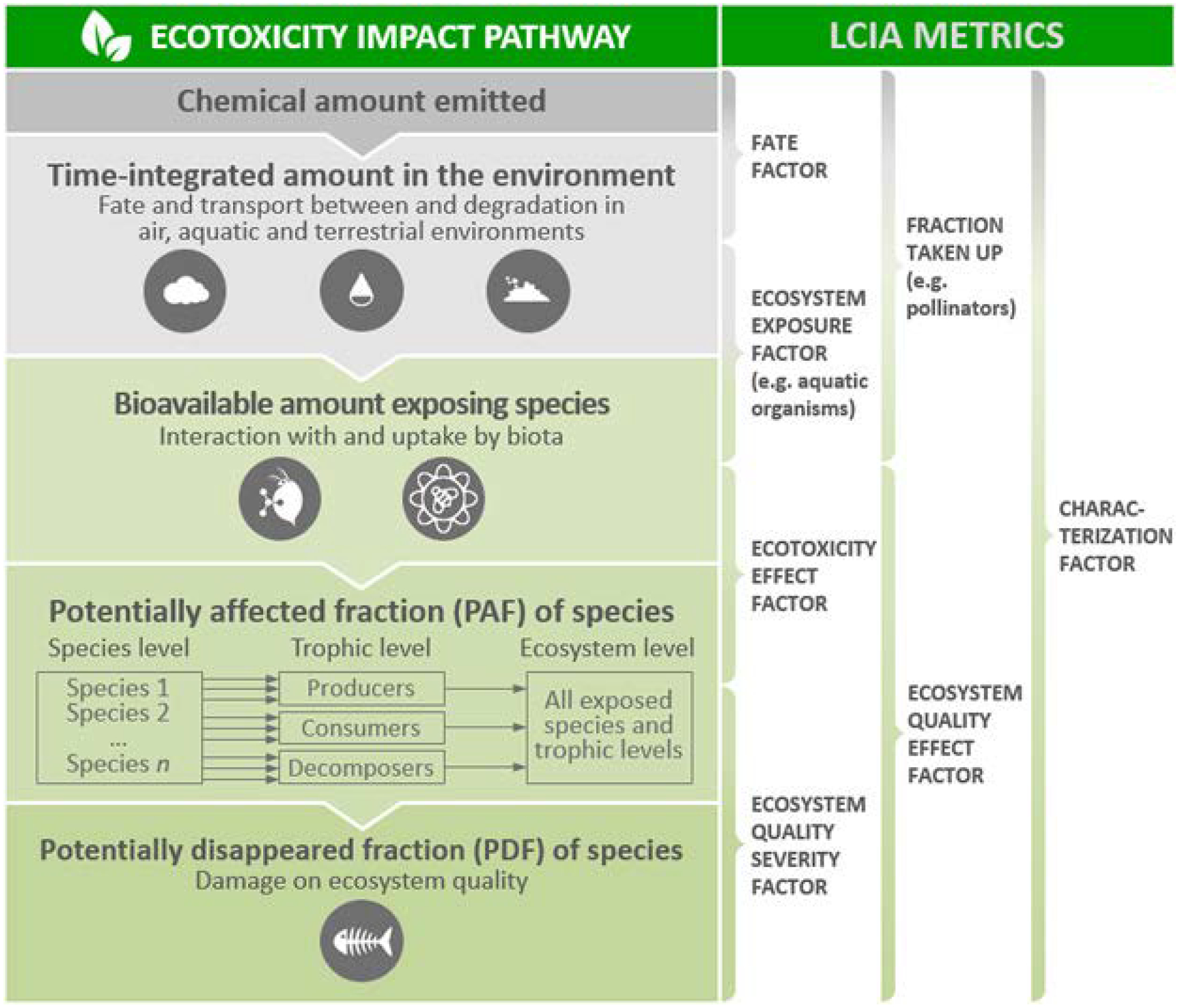
Conceptual representation of ecotoxicity impact pathway in life cycle impact assessment (LCIA). Units of LCIA metrics and the organisms that are considered may differ according to the modeled impact pathways, for example, freshwater ecotoxicity refers to all related organisms across trophic levels using bioavailable chemical mass in freshwater as effect starting point.

In an earlier Life Cycle Initiative effort, available ecotoxicity assessment models were compared and harmonized based on predefined criteria, representing their scientific quality and coverage of impact pathways (Hauschild et al. 2008; Westh et al. 2015). This effort provided expert guidance on central elements of modeling ecotoxicological impacts at dedicated workshops on effect indicators (Jolliet et al. 2006) and fate and effect modeling for metals (Ligthart et al. 2004). A key outcome, endorsed by the Life Cycle Initiative, was the scientific consensus model USEtox (Rosenbaum et al. 2008), which was proposed in 2008 together with the USEtox‐based LCIA ecotoxicity characterization factors for freshwater aquatic ecosystems (Rosenbaum et al. 2008; Henderson et al. 2011). At the time, only the assessment of ecotoxicity in the freshwater compartment was considered sufficiently mature and supported by an adequate amount of test data to allow an appropriate and robust representation of ecotoxicity in LCIA. A later expert consultation on best practice for ecotoxicity assessment of metals (Diamond et al. 2010) led to a modification in the modeling of metal‐related ecotoxicological impacts in freshwater (Gandhi et al. 2010; Dong et al. 2014).

The need for global guidance and harmonization

Since its release, USEtox has been widely used by LCA practitioners. The European Commission recommends it as a reference model to characterize human toxicity and freshwater aquatic ecotoxicity impacts from life cycle chemical emissions for the International Reference Life Cycle Data System Handbook (European Commission 2011b) and the Product Environmental Footprint/Organizational Environmental Footprint (PEF/OEF) pilot phase (European Commission 2013). Despite the consensus on USEtox, stakeholders still debate the appropriate methods for characterizing ecotoxicity in LCIA. Both conceptual and practical challenges drive the debate. There are 2 conceptual challenges. First, impacts need to be estimated for an inherently complex technical and natural system, namely, thousands of chemicals (in contrast to most other LCIA impact categories), which may occur in various environmental compartments (implying different degrees of exposure and sensitivity of exposed species). Second, associated impacts must be estimated or extrapolated from limited data for ecotoxicological endpoints, often measured only under laboratory conditions. Practical challenges arise from variation among chemicals in the empirical data available to characterize ecotoxicological impacts (from no data to hundreds of data points). As a result, different regulatory frameworks use different methods to judge data accuracy and validity. Comparisons with risk and safety assessment approaches have revealed that additional challenges for practitioners are large uncertainties for ecotoxicity characterization factors and the lack of clarity in interpreting USEtox steady‐state ecotoxicity characterization factors (van Zelm et al. 2007, 2009; Saouter et al. 2011; Van Hoof et al. 2011; European Centre for Ecotoxicology and Toxicology of Chemicals 2016).

The conceptual and practical complexities, combined with the demand for decision support, motivate continuous efforts to improve ecotoxicity characterization methods and data, and continued evaluation of recommendations to accommodate new substances being introduced into the market. During the PEF/OEF pilot phase (2013–2017), 25 different European Union industry sectors employed USEtox. The testing phase evaluation revealed that USEtox can lead to results for PEF/OEF that might be difficult to understand and interpret. Based on these conceptual, practical, and interpretation challenges, the PEF/OEF Steering Committee concluded that ecotoxicity could only become a mandatory impact category for assessing, comparing, and communicating the environmental footprint of products or organizations after the implementation of various improvements, ranging from scientific underpinning to interpretation and communication of ecotoxicity results.

Although the available version of USEtox constitutes a useful starting point, scientific advances since its first release in 2008 provide a timely opportunity to review and update guidance for addressing the ecotoxicity of chemicals in LCIA. Ideally, we provide LCA practitioners with tools to address all potential impacts on ecosystem quality, instead of a narrow focus on a very limited set of impact categories (Molander et al. 2004). This requires the pursuit of further scientific development, harmonization, consensus building, communication, and training by improving the process of ecotoxicity‐related exposure and effect modeling (Rosenbaum et al. 2008; Henderson et al. 2011), and specifically addressing the ecotoxicity of metals in freshwater systems (Dong et al. 2014). Our proposed revisions are guided by mature state‐of‐the‐science in environmental exposure and ecotoxicological effects assessment.

Recognized priority issues thus include: 1) exposure of marine biota (Dong et al. 2016) and terrestrial organisms (Owsianiak et al. 2015; Plouffe et al. 2016; Tromson et al. 2017); 2) pollinator exposure and ecotoxicity of pesticides (Crenna et al. 2017); 3) ecosystem impacts via secondary poisoning (Elliott et al. 1997; Nendza et al. 1997; Hop et al. 2002); 4) using ecotoxicological endpoint data and metrics from up‐to‐date and comprehensive data sources (Müller et al. 2017; Saouter et al. 2017a, 2017b; Wender et al. 2018) covering substance classes that are currently not considered in LCIA, such as inorganic salts (Müller and Fantke 2017); 5) combined exposure to multiple chemicals (de Zwart and Posthuma 2005; Backhaus et al. 2013); 6) sediment‐dwelling organisms (Pu et al. 2017); 7) essentiality of certain metals at concentrations below toxicologically relevant levels (Stumm and Morgan 1995; Chapman and Wang 2000; Chapman et al. 2003); and 8) evolution in the bioavailability of metals and other persistent substances (Lebailly et al. 2014; Fantke et al. 2015; Shimako et al. 2017). Our proposed review also considers the availability of the required substance data and gives priority to approaches that are consistent with data and scientific approaches used in other contexts, such as regulatory risk assessment.

Addressing these issues can make ecotoxicity characterization in LCIA more comprehensive and improve support for decision makers who rely on LCIA. The role of the present review is to guide this improvement process and identify related research needs.

Boundary conditions for ecotoxicity characterization

Any updates to LCIA ecotoxicity characterization must respect the boundary conditions of LCA to ensure the relevance and consistency of environmental impact comparisons among different products or services, life stages, and other impact categories. In Textbox 1, we identify 5 boundary conditions of importance to the characterization modeling of ecotoxicological impacts.

TEXTBOX 1: Boundary conditions for characterizing ecotoxicity impacts in life cycle impact assessment.

• The focus of LCA on a functional unit means that the assessment of impacts must be aligned with an emitter or producer perspective (Fantke and Ernstoff 2018; Guinée et al. 2017).

• In following the emitter perspective, ecotoxicity factors depend on substance emissions obtained from the inventory analysis phase of LCA. The inventory information consists of quantified emission flows expressed in kg emitted/functional unit and represents the marginal increase in emissions mass aggregated across the whole life cycle of the studied system(s). Apart from a specification of the primary emission compartment (e.g., air, water, soil), there is limited geographical and temporal specification for most of the quantified emission flows. This makes it difficult to relate the calculated impacts to environmental carrying capacities or similar thresholds, unless spatiotemporally explicit information becomes available at the inventory (e.g., emission patterns) and impact assessment level (e.g., species richness and vulnerability patterns).

• The purpose of LCA is to express the potential environmental impacts and damages associated with a product or service system in a way that supports comparisons between alternatives, both at the level of the individual substance emission and at the level of the entire system under study. To avoid introducing bias in LCA comparisons, LCIA focuses on representative or typical conditions in the modeling of the impact pathways, avoiding worst‐case assumptions used to ensure safety in activities such as premarket regulatory assessments of chemicals.

• The aggregation of the impact scores across the full life cycle and across chemicals requires LCIA characterization scores that are additive—an approach common for other types of impacts characterized in LCIA (Verones et al. 2017).

• It must be possible to quantitatively relate impact scores to damage to the functioning of natural ecosystems and expressed as potential biodiversity loss (e.g., the potentially disappeared fraction of exposed species). At the damage level, results should be consistent with results from other impact categories affecting the same area of protection, that is, ecosystem quality.

In working toward these boundary conditions, we followed a consensus‐building process similar to the approach used to build USEtox. We returned to the fundamental recommendations and principles of USEtox for evaluating all recommendations to update and extend currently used data and methods (not necessarily limited to USEtox). Where useful, we provide additional clarifications for interpreting results in terms of LCIA decision making.

KEY QUESTIONS

An initial Framing Workshop was organized back to back with the Society of Environmental Toxicology and Chemistry Conference in Brussels, Belgium, in May 2017. For this workshop and the overall harmonization effort, a broad range of internationally recognized scientists and practitioners in environmental exposure and effect modeling was brought together, to obtain state‐of‐the‐science models and data.

The specific objectives of our effort were to first identify and discuss the main scientific questions and challenges to an improved framework for characterizing potential ecotoxicological impacts on ecosystems from exposure to chemicals, and also to provide initial guidance to the process. A set of key questions was identified and discussed in terms of 3 broader topics: 1) approaches and data needed to determine ecotoxicity indicators for chemical emissions; 2) the validity and maturity of approaches and data needed to represent ecotoxicological impacts in environmental compartments other than freshwater; and 3) the relevance and feasibility of specifically improving the ecotoxicity characterization of metal emissions including essentiality and long‐term dynamics. We summarize the questions in Textbox 2 and discuss the outcomes in detail in the following sections.

TEXTBOX 2: Key questions for advancing and harmonizing the current ecotoxicity characterization framework in life cycle impact assessment.

1. General assessment framework

   • Can we use as a starting point the framework that is a result of earlier scientific consensus‐building efforts (Hauschild et al. 2008; Rosenbaum et al. 2008) to include the broad range of ecotoxicological impacts from chemical emissions into LCIA and to improve the underlying data basis, given the boundary conditions posed by LCA
   • What is currently missing from the existing framework regarding environmental compartments, impact pathways, exposed organisms, or new ecotoxicity data, allowing for aggregating over chemical substances, and levels of spatiotemporal detail?
2. Additional compartments, exposed organisms, and impact pathways

   • How can we include additional ecotoxicity‐related impact pathways, exposed organisms, and environmental compartments based on available evidence and data?
   • Marine water: What data can be used for ecotoxicity to marine organisms; which approaches exist to supplement freshwater ecotoxicity data and what is the level of maturity; and is there a need to subdivide the marine compartment (e.g., distinguishing coastal waters from open ocean) and if yes, how can we do it?
   • Sediment: What models and data can be used for sediment‐related fate processes and ecotoxicity to sediment‐dwelling organisms; which approaches exist to supplement freshwater ecotoxicity data and what is their level of maturity; and what is the added value of including sediment, if aquatic and potentially also terrestrial species are already considered?
   • Groundwater: What models and data can be used for groundwater‐related fate processes and ecotoxicity to groundwater organisms; which approaches exist to supplement freshwater ecotoxicity data and what is their level of maturity; and what is the added value of including groundwater, if aquatic species are already considered?
   • Terrestrial soil: What data can be used for ecotoxicity to soil organisms and what is their level of maturity; and which approaches exist to supplement freshwater ecotoxicity data with data specifically for soil organisms?
   • Other terrestrial organisms: What impact pathway approaches will have to be modeled; which models and data can be used for ecotoxicity; and what is their level of maturity for 1) pollinating and nonpollinating insects, 2) birds, and 3) predators via food chain biomagnification and secondary poisoning?
3. Metrics for ecotoxicity characterization in LCIA

   • Which metric is most appropriate for modeling toxicity‐related effects on ecosystems in LCIA, taking into account: 1) the relevance of the metric for predicting ecosystem damage in the form of potential biodiversity loss, 2) the uncertainty of the metric, and 3) the boundary conditions of LCA, notably the aim of comparing alternative solutions based on characterization results across different impact categories?
   • What are the major studies we need to take into account to determine concentration–response functions for different organisms for the relevant ecosystem effect endpoints; are there any emerging studies that could be used as alternatives to our default linear approach; and are there recent developments in other impact categories contributing to impacts on ecosystem quality where nonlinear approaches are used?
   • What are important data sources for relevant ecotoxicological effect metrics?
   • What is best practice for extrapolation from acute to chronic effects and between levels of acute and chronic effects?
   • What is the best way to compare chemical ecotoxicity? Is there a need to align with global regulatory practices and, recognizing that data availability varies among chemicals, is it more important either to treat all chemicals the same way or to ensure that the most toxic chemicals are reliably characterized in LCA?
   • How should chemical mixtures in the environment and mixture toxicity be handled, that is, combined exposure to multiple chemicals from the same emission source or from the background chemical mixture resulting from processes outside the product life cycles of alternative solutions?
   • Which empirical insights exist on damage to ecosystem structure and ecosystem functioning (relevant for ecosystem services) due to exposure to chemicals, and what are the relevant mechanisms and which indicators describe them best?
   • Which empirical and mechanistic insights exist on the disappearance of species from an ecosystem due to chemical exposure and what is the maturity of available approaches and data?
4. Ecotoxicity modeling for metals

   • With respect to essentiality, when certain emitted metals occur below toxicologically relevant levels, what is the relevance for different ecosystems; which metals are essential for which organisms; and what is the variability of essentiality concentrations between individual organisms?
   • With respect to long‐term ecotoxicity of metals, how does the speciation and accessibility of metals change over long time periods in marine and terrestrial environments with respect to: 1) patterns for different metals, 2) dynamic modeling, 3) influence on bioavailability, and 4) differences to freshwater compartments?
   • How can dynamic aspects (changes in mass distribution over time) related to the environmental fate of metals be considered in ecotoxicity characterization?

GENERAL ASSESSMENT FRAMEWORK

We consider the current framework in LCIA (Rosenbaum et al. 2008; Henderson et al. 2011) a suitable starting point for assessing ecosystem damages from emissions of toxic chemicals. In this framework, the focus is on determining the potential fraction of species lost in aquatic ecosystems due to chemical emissions, based on the modeled relationship between chemical exposure mass in the environment and the potentially affected fraction (PAF) of species. This relationship is based on a statistical model, which describes the variability across species in their sensitivity to a chemical, based on data collected from various ecotoxicity databases and including no‐observed‐effect concentrations (NOECs), various effect concentration (ECx) values, or various lethal concentration (LCx) values obtained in laboratory toxicity tests with single chemicals and single species. This model is known as the species sensitivity distribution (SSD) model and expresses the PAF of species exposed at the level above the ecotoxicity endpoint of the model (Posthuma et al. 2002).

Various studies have shown that the impact of chemicals based on an SSD model, especially SSD_EC50 based on reported or extrapolated median effect concentration (EC50) data, can be empirically related to ecosystem damage quantified as loss of taxa (Posthuma and de Zwart 2006, 2012; Posthuma et al. 2016). This step represents the “translation” of the dimensionless PAF outcome to the field‐relevant quantification of fraction of species lost (potentially disappeared fraction [PDF]). In USEtox and in LCIA generally, this model and its validation have been used to derive ecotoxicity‐related impacts on freshwater ecosystems. However, although LCIA characterizes potential ecotoxicological impacts associated with a product or service life cycle using PAF and PDF as metrics, this does not imply actual species loss in a particular environment, for which site‐specific emission, exposure and effect estimates would be required. These impacts described by a characterization factor, CF_c (PDF m³ d/kg_{emitted in c}), are finally complemented by a severity factor (SF) to relate PAF to the level of damage imposed on ecosystem quality expressed as potential species loss (Fantke et al. 2017):

$${\text{CF}}_C={\text{FF}}_{w\leftarrow c}\times {\text{XW}}_F\times {\text{EF}}_w\times \text{SF}$$ (1)

where FF_w←c (kg_{in w}/kg_{emitted in c} /d) denotes the steady‐state fate factor from compartment c to freshwater w; XF_w (kg_{dissolved in w}/kg_{in w}) denotes the truly dissolved (metal ions) or total dissolved (organic substances) fraction of chemical mass in freshwater; EF_w (PAF m³/kg_{dissolved in w}) denotes the ecotoxicological effect factor linking the PAF of freshwater species integrated over exposed water volume and time to the truly dissolved chemical mass in freshwater; and SF (PDF/PAF) denotes the severity factor expressed as relationship between the PDF of species and the PAF. SF expresses the severity of exposing the ecosystem species to the effect concentrations considered in the determination of EF, where the concentration is estimated from emitted mass and an assumed compartment volume. The FF_w←c can be interpreted as the product of the residence time of a chemical in freshwater, FF_w←w (d), and the overall time‐integrated mass fraction transferred from emission compartment c to freshwater, f _w←c (kg_{in w}/kg_{emitted in c}):

$${\text{FF}}_{w\leftarrow c}= \text{F}\stackrel{f_{w\leftarrow c}}{\overbrace{{\text{F}}_{w\leftarrow c}/{\text{FF}}_{w\leftarrow w}\times {\text{FF}}_{w\leftarrow c}}}$$ (2)

Introducing PAF and PDF with the stated units makes it clear that characterization results refer to a particular fraction. In this case, the fraction of exposed species in the entire exposure compartment over the given chemical residence time in that compartment that either experiences exposure above their species‐specific effect concentration (in case of PAF) or that potentially disappears (in case of PDF). However, using these species fractions as part of the impact factor also brings difficulties in the interpretation among stakeholders and needs to be further discussed.

This mathematical framework is also generally applicable to the characterization of ecotoxicity for organisms other than freshwater species, specifically, in line with recent developments, also for marine and soil organisms (Owsianiak et al. 2013, 2015; Dong et al. 2016; Plouffe et al. 2016). Characterization factors can be applied among a set of chemicals to denote the ranked potential of a specific chemical to pose harm to species assemblages. Ecotoxicity characterization is not restricted to direct effects on species assemblages as a starting point for SSDs, which could also make use of the observed vulnerability of specific taxa that have value due to factors such as providing ecosystem services. Hence, an alternate modeling approach may focus on species‐specific population modeling as a basis for damage characterization. For some specific organisms like pollinators (e.g., honey bees), the existing characterization framework needs modification to account for species‐specific exposure/effect data rather than the more ecosystem‐level bioavailable mass fractions and related exposure and effect concentrations (Doublet et al. 2015).

In principle, a regionalized effect assessment (e.g., using tropical species for effects in tropical regions) is relevant for all environmental compartments and organisms. Currently applied LCIA characterization models, however, do not include data explicitly applied to specific locations for distinguishing between different species occurrence and effect distributions. Instead, LCIA ecotoxicity modeling is currently based on data available mostly for a few standard test species, some of which are temperate (e.g., Daphnia magna) and some subtropical or tropical (e.g., Danio rerio). As long as the available ecotoxicological data only reflect effects on a few standard species, ecotoxicological assessments cannot be made spatially explicit. Recent work, however, indicates that the sensitivity of tropical ecosystems may potentially be approximated by data from common (temperate and tropical) test species (Daam and Van den Brink 2010). Additional challenges are unique ecosystems in the tropical regions that are not well represented by processes included in current LCIA fate models (e.g., mangroves and coral reefs). Considering the state‐of‐the‐science and scarcity of effect data, regionalization of ecotoxicity impact pathways in LCIA requires further research before it can be integrated in currently applied models. We recommend summing up effect results across chemicals, which is the current default in LCIA, as a first approximation for handling mixture toxicity under the typical situation of unknown chemical emission location and time along product life cycles. However, the multisubstance PAF approach, which builds on aggregating predicted impacts across substance groups with (dis)similar modes of action (de Zwart and Posthuma 2005), should be further explored.

ADDITIONAL COMPARTMENTS AND PATHWAYS

Since the release of USEtox in 2008, practitioners and stakeholders have requested an extension of ecotoxicity characterization beyond freshwater environments. Several efforts have explored the possibility of including other compartments and have resulted in emerging models supporting the assessment of fate, exposure, and ecotoxicological effects in marine, terrestrial, and sediment environments (Owsianiak et al. 2015; Dong et al. 2016; Plouffe et al. 2016; Crenna et al. 2017; Pu et al. 2017). Guidance is needed on whether these models and their underlying data are already mature enough for inclusion into LCIA. In the following, we mainly focus on impacts on freshwater and marine mammals and birds; we also discuss sediment‐dwelling and groundwater organisms, as well as impacts on the terrestrial environment, pollinating insects, predatory birds, and other land animals.

Warm‐blooded organisms

Certain lipophilic chemicals may accumulate in biota and be transferred within the food chain, leading to exposure of organisms at higher trophic levels, such as mustelids and predatory birds. This is already considered in existing LCIA methods. However, ecotoxicity characterization results differ among available methods, especially for substances that are bioaccumulative (Mattila et al. 2011). Bioaccumulation can occur in all aquatic and terrestrial food chains and across cold‐blooded and warm‐blooded species, but research has shown that uptake from food is particularly important for warm‐blooded predators (Kelly et al. 2007). A study of the ecotoxic impacts of chemicals on warm‐blooded predatory species, however, has found that a high relative impact on cold‐blooded species, primary producers, and decomposers does not necessarily indicate a high relative impact on warm‐blooded predators (Golsteijn et al. 2012b). However, this effect might be different for metals, for which studies have shown that sources of bioaccumulation differ across the metals, demonstrating the importance of investigating upper and lower trophic levels separately to fully understand metal transfer pathways in aquatic and terrestrial food webs (Chen et al. 2000; Ouédraogo et al. 2015). We recommend addressing bioaccumulation for warm‐blooded species (and other species) by considering all trophic levels and calculating effect estimates separately for each trophic level, which is consistent with other findings (e.g., Chen et al. 2000; Larsen and Hauschild 2007b). Depending on the weighing of trophic levels, the inclusion of impacts on warm‐blooded predators may influence the relative ranking of chemicals in an LCIA. Because incomplete data are available for many chemicals across trophic levels, data points from available trophic levels are used and averaged, instead of averaging for each trophic level separately.

Marine water

Species diversity and density are much higher in coastal marine waters than in the open ocean. This argues for a distinction between the 2 and the possibility of only including the coastal compartment in LCIA, an approach that was already recommended for metals at the Apeldoorn workshop (Ligthart et al. 2004).

Extremely persistent and mobile chemicals, such as metals and per‐ and polyfluoroalkyl substances, will accumulate in oceans if they are sufficiently water soluble (Prevedouros et al. 2006). To capture the potential effects of persistent chemicals on marine organisms, we suggest considering ecotoxicological effects in marine environments and adding these to the existing framework. Finally, secondary poisoning of birds and mammals could be relevant in relation to exposure from marine ecosystems, but available data for many relevant species are usually lacking (Nendza et al. 1997).

Sediment

Addressing ecotoxicological impacts on sediment‐dwelling organisms (benthic biota) requires the incorporation of an additional compartment into the existing framework. Based on the evaluation of maturity, quality, and availability of existing approaches for addressing sediment in multimedia fate modeling, a sediment compartment is a potentially important addition to the proposed framework, particularly in light of persistent substances with a potential to build up high exposure concentrations in sediments and related organisms. In addition, for certain chemicals such as cyclic siloxanes, sediments provide potential transfer pathways for bioaccumulation (Wang et al. 2013). Required data for including ecotoxicity to sediment‐dwelling organisms are becoming more readily available and could be sufficient to become part of LCIA. If sediment toxicity effects could be estimated by ecotoxicity data for pelagic species (e.g., via equilibrium partitioning for nonpolar organic chemicals), such an inclusion would put a stronger emphasis on sediment‐binding chemicals of concern, as just mentioned. Because aquatic sediment belongs to aquatic ecosystems, we suggest considering effects on benthic and sediment species for integration into 2 overall aquatic ecotoxicity impact scores (i.e., freshwater and marine).

Groundwater

Addressing ecotoxicological impacts on groundwater organisms (stygobiota) requires the incorporation of a separate groundwater compartment, in addition to exposure and effect data for these organisms. We evaluated the availability of approaches addressing groundwater organisms in a multimedia modeling context. Several studies indicate that groundwater organisms have longer life cycles due to lower metabolic rates, greater fat storage, and adaptation to low‐energy environments (Di Lorenzo et al. 2014), and show different sensitivities to chemical exposure (Hose 2005) than phylogenetically related surface‐water species, although similar sensitivities have also been indicated (Verweij et al. 2015). However, the availability of experimental data for toxicity to groundwater organisms is extremely limited, making it difficult to introduce a separate impact pathway at this point. Therefore, the benefit of representing toxicity to organisms in groundwater is a low priority.

Terrestrial soil

Ecotoxicological impacts on soil organisms are relevant for assessing product systems that include pesticide releases, sewage sludge applications, deposition of air emissions, and/or use of irrigation water contaminated by emissions or deposition. We suggest that a detailed analysis of the state‐of‐the‐science to derive recommendations on how terrestrial soil ecotoxicity can be addressed in LCIA. The absence of soil toxicity data could be addressed with the use of aquatic toxicity data to estimate terrestrial soil ecotoxicity based on the sorption‐based equilibrium partitioning between media and phases (van Beelen et al. 2003). For most chemical groups, soil porewater hazardous concentrations are approximately a factor of 3 higher than the respective hazard concentrations in freshwater. However, the large overall statistical uncertainty in deriving multispecies hazard concentrations makes it hard to assess whether there are systematic deviations in such concentrations between aquatic and soil species (Golsteijn et al. 2013). Available studies on soil impacts recommend the use of species samples of different trophic levels with consideration of bioaccumulation (Hop et al. 2002). If the sample size is too small or specific species (e.g., birds) toxicity data are not available, interspecies correlation estimations could provide representative samples (Golsteijn et al. 2012a). We conclude that the consideration of ecotoxicological impacts on terrestrial organisms is needed, but requires further study.

Exposure of pollinating insects and other species of special concern

Among terrestrial aerial species, pollinators are of special concern for their role in providing essential ecosystem services (Kerr 2017; Woodcock et al. 2017). Pollinators are affected by many different stressors, including chemical exposure. Estimating exposure for pollinators, however, is more complicated than starting from concentrations in soil, water, or air. It could be more expedient to link a dose of pesticide applied to agricultural land (usually expressed in kg active ingredient applied/ha) to the probability of effect on pollinators and potentially other species of special concern (Crenna et al. 2017), in analogy to how human exposure to chemicals is estimated. Efforts are in progress to characterize impacts on pollinators, but need to be expanded before they can be included in the existing framework.

DATA AND METRICS FOR ECOTOXICITY CHARACTERIZATION

Data relevant for ecotoxicity characterization

Substance‐related input data, including physicochemical properties, chemical half‐lives, and ecotoxicity effect information in ecotoxicity characterization models like USEtox, should be aligned with the most recently available large data sources. One strong example is the IUCLID database of the European Chemicals Agency (ECHA) used for the Registration, Evaluation, Authorisation and Restriction of Chemicals (REACH) in the European Union. The Joint Research Center of the European Commission and the USEtox International Centre are currently assessing the possible use of REACH registration data as input to USEtox (Müller et al. 2017; Saouter et al. 2017a, 2017b). These efforts are timely, and clear recommendations are needed on how to make effective use of REACH and other data sources for LCIA. This includes addressing data ownership and rights of use. In view of the recent data quality evaluation published by the Umwelt Bundesamt (German Federal Environment Agency 2015), we stress the need for adequate quality control of the data. Considering the available data in various databases, there is ample opportunity to combine the global data collection, and specific novel data collections (such as for REACH), and apply pertinent quality and relevance criteria to strike a balance between needs for decision support (preferred: all chemicals) and precision (preferred: sufficient data quality and quantity).

Exposure metrics

The exposure factor presented in Equation 1 translates the total mass of a chemical in water into the truly dissolved mass to which organisms are exposed. However, multimedia transfer and degradation processes of organic chemicals in the environment are usually based on the octanol/water partition coefficient, whereas for surfactants and similar surface‐active chemicals, other parameters might be better suited, such as hydrophilic–lipophilic balance values. For metals, the exposure factor must represent the truly dissolved fraction of the metal, comprising the free ions (that are normally responsible for the toxicity) and the inorganic complexes within the dissolved phase (Diamond et al. 2010; Gandhi et al. 2010; Dong et al. 2014, 2016). For soils, solid‐phase speciation is relevant for metals because it determines which fraction of the metal pool in the soil is potentially available for leaching and uptake by biota. Thus, for exposure of soil organisms, workshop participants proposed an exposure factor that is either 1) the product of an accessibility factor representing the solid‐phase reactive fraction of total metal in soil, and a bioavailability factor, which determines the fraction of the reactive metal pool that is present in immediately bioavailable metal forms (Owsianiak et al. 2013, 2015); or 2) the ratio between bioavailable and total metal mass (Plouffe et al. 2015). These metrics should be considered as best available options for use in LCIA. However, the main issue in implementing these metrics is how to model them consistently for the different aquatic and terrestrial compartments. This needs to be included in the discussion of the modeling of the effects on the ecosystems of the individual compartments.

Effect metrics

The ecotoxicological effect factor as currently used in USEtox, EF_w (see Equation 1), represents the potential toxicity of any chemical emission flow to the exposed freshwater aquatic ecosystem and is based on an indicator of the chronic toxicity of the substance to (ideally) all species of that ecosystem (Henderson et al. 2011). Chronic ecotoxicity is considered most relevant for LCA when the focus is on long‐term exposures from processes in a product system rather than short‐term high‐concentration pulses with acute effects. The focus on chronic ecotoxicity corresponds well with the current fate factor component of the characterization factor, which is based on the modeling of a change in steady‐state concentration resulting from a change in emission flow. The choice for the current approach in ecotoxicity characterization (by USEtox and other prevailing characterization models like USES‐LCA and IMPACT2002+) can give rise to results that are dominated by metals and highly persistent chemicals, while more short‐lived (and potentially quite toxic) organic compounds recede from interest. This chemical focus and ranking may differ from environmental hazard ranking and risk assessment.

Chronic toxicity is estimated from observations of the sensitivities of a subsample of the species of which an ecosystem might be composed. The approach is based on confirmation studies, in which it has been shown that an increase in the predicted fraction of species that is potentially affected (PAF based on SSDs) for a chemical is related to an increased ecological effect (van den Brink et al. 2002; de Zwart 2005; Posthuma and de Zwart 2006, 2012). Recommendations from ongoing efforts in other task forces of the GLAM project suggest that PDF should be used as a default damage level metric, given its prevalence in the other impact categories that affect ecosystems (e.g., acidification). However, the PDF must be clearly defined to ensure that damages can be compared across impact categories (Verones et al. 2017).

Sensitivity observations needed to derive the ecotoxicological effect indicator are composed of the set of available test results. These tests are commonly laboratory experiments exposing test organisms from different trophic levels in the ecosystem to the chemical under controlled and reproducible conditions in preferably standardized conditions. Various global or regional databases contain substantial amounts and types of data, reflecting data that are traceable to published scientific literature or to regulatory registration requirements (e.g., REACH). The combined data sets contain approximately 1 million test outcomes (partly representing copied entries). A selection must be made from the available toxicity data, which may represent acute or chronic exposure relative to the life cycle of the organism (temporal aspect) or no‐, low‐, or median‐response endpoints (e.g., ECx as the effect concentration that elicits effect in x % of the exposed organisms compared with the background). An overview of ecotoxicological effect data for freshwater organisms reported under REACH for different endpoints and species groups is given in Figure 2, which is adapted from Saouter et al. (2018). After data cleanup (e.g., removing double entries and entries without reporting exposure duration), 146 817 data points ended up in acute and chronic categories based on reported exposure duration.

Figure 2.

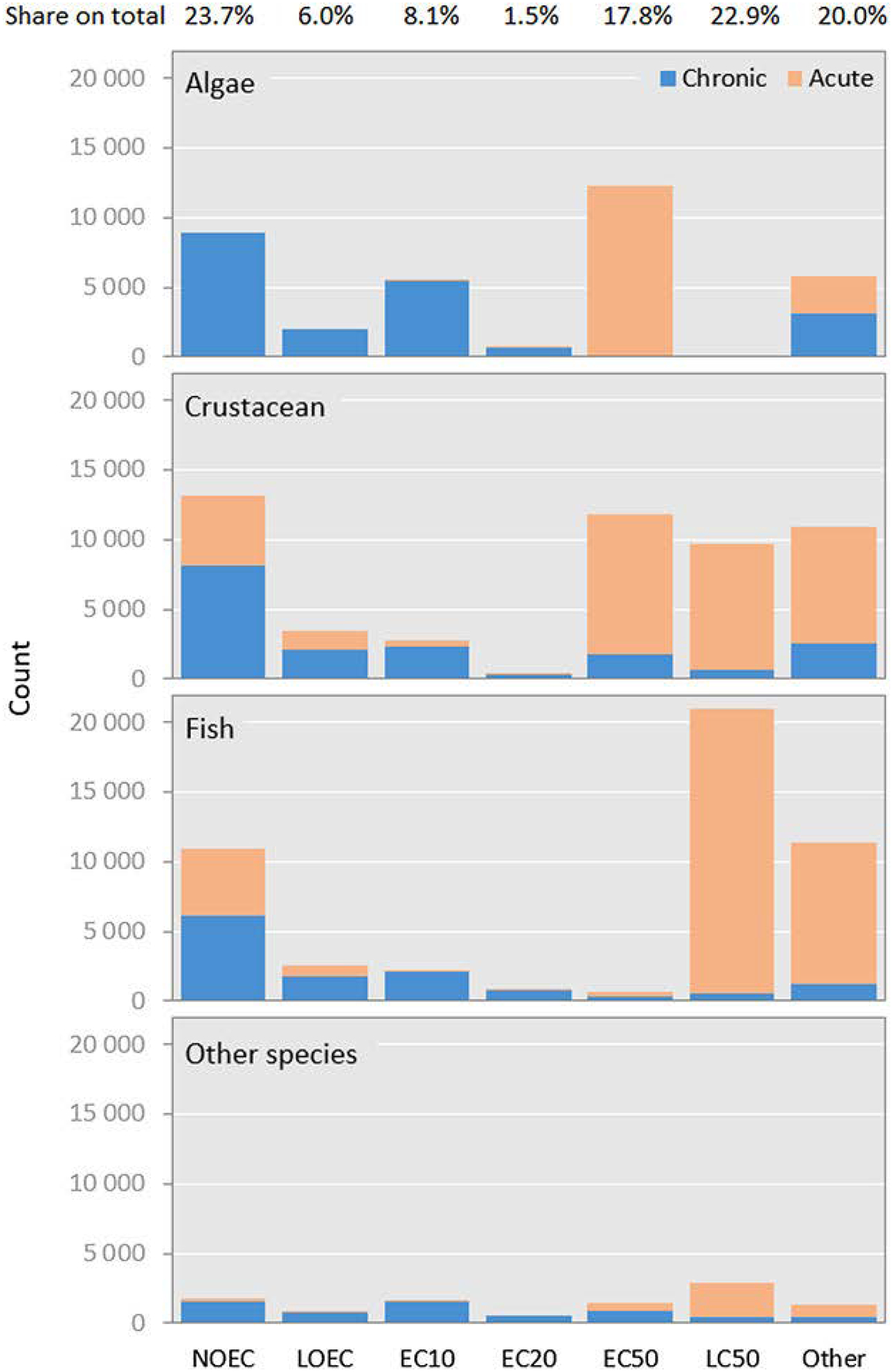
Number of acute and chronic ecotoxicological effect data available in the Registration, Evaluation, Authorisation, and Restriction (REACH) regulation for the species groups algae, crustacean, fish, and other species (includes amphibian, anellidae, insect, mollusca, plant, and rotifera) and endpoints. NOEC = no‐observed‐effect concentration; LOEC = lowest‐observed‐effect concentration; EC = effect concentration; LC = lethal concentration; Other = contains all endpoints not listed separately and includes, for example, EC5 and EC100), and the share of endpoints on the total data count (n = 146 817).

To represent possible chronic impacts of a chemical on an ecosystem in the effect factor, preference might be given to results from chronic or subchronic tests at a meaningful ECx level (Jolliet et al. 2006; Larsen and Hauschild 2007a). When the needed chronic/subchronic endpoint data are not available but other endpoint data exist, extrapolation routines can be applied to estimate chronic responses from acute data and to estimate response levels with scare data (e.g., EC10 or EC50) from other levels—such as NOEC. This is supported by Figure 2, which shows that chronic data are mostly reported at NOEC, LOEC, and EC10 levels, together accounting for 75% of all reported chronic data in REACH, whereas acute data are mostly available at EC50 and LC50 levels, together accounting for 61% of all reported acute data in REACH.

After collating test results for the chemical across different test organisms, the SSD curve can be constructed (Posthuma et al. 2002); this curve depicts the fraction of species in the ecosystem that are affected above their chronic ECx value (y ‐axis) as a function of the truly dissolved concentration (x ‐axis) of the chemical. Figure 3 provides illustrative examples of SSD curves. The SSD models may be constructed from ecotoxicity tests in which the ECx is observed, from NOECs, or from any other relevant subset of relevant data. Figure 3 shows SSDs derived from a data set provided by ECHA, composed of 188 data points covering 3 relatively data‐rich substances. In this set, 19 data points had to be excluded, mainly due to noninterpretable information about test duration, effect endpoint, unit or species tested. After the data cleanup, the median of the remaining data points for each substance–species combination was derived for EC50 and NOEC data, respectively, as example metrics. We note that SSDs describe data sets, which can be fully characterized by a median and a standard deviation and in theory from 2 data points, whereas a higher number of data improves model reliability.

Figure 3.

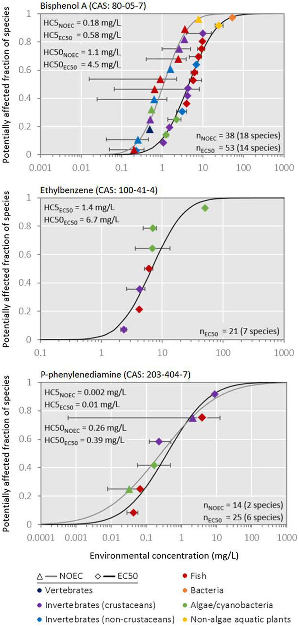
Cumulative species sensitivity distribution (SSD) functions of reported chronic no‐observed‐effect concentrations (NOECs) and chronic concentrations affecting 50% of exposed individuals (EC50) for each species included in the cumulative distribution for 3 chemicals with varying data availability, and related minimum–maximum error ranges and geometric means across data points for 5% (HC5) and 50% (HC50) of affected species. With such data, we can study per species extrapolation (acute‐chronic) when needed, but also SSD‐to‐SSD extrapolation, to obtain the desired SSD_EC50 from other available data, where the latter is often robust, implying a shift of the SSD_x to SSD_EC50.

The ecological relevance of the model also increases when the test data better represent the assemblage of species exposed in the field. Formal data requirements for the derivation of protective benchmark concentrations exist and vary among jurisdictions; often, ecotoxicity data for 5 to 10 species across taxonomic rank at the family level are deemed necessary (Nugegoda and Kibria 2013). For example, data on at least 8 to 10 families are required in the European Union and the United States (European Commission 2011a; US Environmental Protection Agency 1985), whereas specific modes of action are proposed to result in deriving and using separate models for sensitive and insensitive taxonomic species groups (e.g., European Food Safety Authority 2013). This issue is illustrated in Posthuma et al. (2002). Note further from Figure 3 that one (predicted or measured) ambient exposure level implies the presence of a suite of different impacts in different species. That is, 1 mg/L of bisphenol A (top panel of Figure 3) can be interpreted—shown by the curves—as 10% of the species being exposed beyond their EC50, as well as simultaneously 50% of the species being exposed beyond their NOEC. The hazardous concentration at which 50% of a population dies (HC50_EC50) is to be considered a summary metric, derived from inter‐species differences in sensitivity, which empirically relates to species loss, but which also is a summary of a field‐SSD of effect levels. Notably, in the derivation of protective regulatory water quality criteria for chemicals, metrics like HC5 or HC10 are used, in which case with an SSD based on NOECs, that is, HC5_NOEC or HC10_NOEC (see Part II of European Commission 2003), where the choice of the underlying data (e.g., NOEC, EC5, EC10, EC20) does not seem to largely affect HC5 or similar summary metrics (Azimonti et al. 2015; Iwasaki et al. 2015). The SSDs shown in Figure 3 for selected chemicals can also be constructed from data for many other substances if they are available.

The purpose of LCA, and hence of characterization modeling in LCIA, is to compare alternative products or product systems rather than to risk or impact on an absolute scale (Ligthart et al. 2004; Jolliet et al. 2006). Following previous work and recommendations on the choice of the LCIA ecotoxicity indicator, priority should be given to the use of statistically robust yet ecologically relevant measures of toxicity rather than protective measures of toxicity, which are generally interpolated in the lower tail of the SSD distribution and reflect an exposure related to “unlikely impacts.” The effect factor in USEtox is currently based on the HC50_EC50, defined as the geometric mean of EC50s across species (Fantke et al. 2017), rather than being based on the HC5_NOEC or the predicted no‐effect concentration (PNEC) used in preventive regulatory assessments. The PNEC is typically derived from the toxicity data for the most sensitive tested species, divided by an assessment factor to ensure protection of the ecosystem. The HC50_EC50 reflects the average sensitivity of all species of the ecosystem at the EC50 level rather than the most sensitive species. It can be seen from the 3 SSD curves in Figure 3 that the ratio between HC50_EC50 and HC5_EC50 varies between chemicals—for example, from 4.8 for ethylbenzene to 39 for p ‐phenylenediamine. This reflects the different shapes of the SSD curves, in turn related to a data‐poor comparison (p ‐phenylenediamine: only 2 NOEC data points resulted in the flat SSD). However, experience shows that shifts between SSD curves of different endpoints across chemicals are rather robust, allowing approximation and across‐SSD_type extrapolations, for example, from SSD_acute to SSD_chronic, or vice versa. The recognition of this pattern in SSDs dates back to de Zwart (2002), and this approach may be a basis for seeking improvements to the characterization of ecotoxicity in LCIA.

The effect factor for freshwater ecotoxicity, EF_w (PAF m³ d/kg), is currently defined as (Rosenbaum et al. 2008; Gandhi et al. 2010):

$${\text{EF}}_{\text{w}}=0.5/\text{HC}{50}_{\text{EC}50}$$ (3)

where 0.5 denotes the 50% level of species that are potentially affected above their EC50 (PAF) and HC50_EC50 (kg/m³) refers to the effect indicator calculated as the geometric mean of available chronic EC50s for species of the affected ecosystem. Because we want EF to represent the slope of the curve connecting the origin and the midpoint, it has to be the midpoint value of the y ‐axis (0.5) divided by the midpoint of the x ‐axis (HC50). However, EF can be defined in different ways, with each eventually summarizing the ranked position of a chemical in terms of posing harm to species assemblages. The EF metric choice matters, for both technical aspects (data availability, alignment with other PDF definitions in LCIA) as well as communication aspects (protective chemical risk assessments utilize HC5_NOEC, so that deviating choices require specific communication). In terms of the constraints and characteristics of the boundary conditions of the assessment of ecotoxicity in LCIA, Table 1 summarizes the strengths and weaknesses of the different options for deriving effect factors (based on different concentration–response metrics); a similar analysis was performed and is discussed in Saouter et al. (2017a).

Table 1.

Characteristics of options for ecotoxicological effect factor^a

Effect factor (concentration–response metrics)	Ecosystem impact representativeness	Robustness and sensitivity to number of experimental data points	Uncertainty and ease of application
0.5/HC50EC50(b)	Effect oriented, accounts for all possible effects and related species sensitivities	Most robust between data‐rich and ‐poor chemicals Premodeling split in SSD for sensitive taxa (e.g., insecticides with separate SSDs for insects and noninsects) would have high numerical effect	Uncertainty can be estimated using bootstrap methods Recommended earlier for comparative life cycle assessment (Jolliet et al. 2006; Pennington et al. 2004)
0.05/HC5EC50	Effect oriented, accounts broadly for effects and species sensitivities	More influenced by the shape of the curve Sensitive to number of species tested Premodeling split in SSD for sensitive taxa (e.g., insecticides with separate SSDs for insects and noninsects) would have low numerical effect	Higher uncertainty than HC50, but higher “protection” level
0.05/HC5NOEC or 0.1/HC10NOEC or 0.2/HC20NOEC(b)	No‐effect oriented, that is, cannot be directly used to predict effects and related species loss as such	Influenced by tested concentrations, not the shape of the curve More sensitive to number of species tested	Uncertainty higher than for EC50‐based HCs due to its unknown distance to the (true) LOEC Recommended for protective chemical risk assessment if data available (European Commission 2003); allows for use of chronic NOEC data that can be extrapolated to EC10, for example, given that the choice of ECx level (e.g., EC5, EC10, EC20) or NOEC does not largely affect HC5 or similar summary metrics (Azimonti et al. 2015; Iwasaki et al. 2015)
1/PNEC concentration–response based on most sensitive species	No‐effect oriented, cannot be directly used to predict effects and related species loss	Very sensitive to number of species tested Bias between emerging substances with 3 tests and well‐studied chemicals (such as metals) Not intended for comparative effects assessment	Commonly used in protective chemical risk assessment and environmental quality assessment Conservative (especially when additional “safety factors” are introduced) Based on key chemical safety studies (e.g., under the European REACH regulation)
All metrics	No consideration of keystone species and ecological interactions Chronic data often based on acute‐to‐chronic extrapolations

^aText in italics are statements relative to the current approach using 0.5/HC50_EC50

^bPotentially best suited as ecotoxicity effect metric in LCIA based on additional study.

HC50 = hazardous concentration at which 50% of a population dies; 0.5/HC50_EC50 = 50% level of species that are potentially affected above their median effect concentration (EC50); SSD = species sensitivity distribution; NOEC = no‐observed‐effect concentration; LCIA = life cycle impact assessment; LOEC = lowest‐observed‐effect concentration; PNEC = predicted no‐effect concentration; REACH = Registration, Evaluation, Authorisation and Restriction of Chemicals.

The motivations for choosing the 50% effect level are, among others, the statistical robustness of determining the concentration corresponding to the 50% response level (positioned in the middle of the concentration–response curve), and also the possibility of translating the exposure into disappearance of species, because exposures above EC50 can be related to disappearance observed in field‐exposed ecosystems (Posthuma and de Zwart 2006, 2012). However, this endpoint is not routinely generated; for historical reasons, preference in testing has been for chronic NOEC‐type endpoints and acute EC50s. Hence, we need to find a way to tap into the existing chronic data (e.g., NOEC, EC10) for use in LCIA. Other effect response levels (e.g., EC10, EC20) might be an alternative option for deriving effect factors because they are closer to the range where chronic data are routinely generated (i.e., chronic NOEC). In addition, EC10 data are more in the range of environmentally relevant substance concentrations. Given these conditions, different effect levels should be tested to evaluate the tradeoff among availability of chronic data, statistical robustness, and environmental relevance of concentrations.

Damage metrics

In an effort to match an ecosystem impact metric with the LCA boundary conditions stated in Textbox 1, the focus should be on impact scores that can be quantitatively related to damage imposed on the structure of natural ecosystems and expressed as biodiversity loss (Larsen and Hauschild 2007a) or as damage to populations of individual species (such as bees). This brings the ecotoxicity indicator in line with damage level indicators from other impact categories that also relate to ecosystem quality and facilitate grouping or comparing across impact categories. To meet this goal, indicator scores expressed in the PAF (of species) must be translated into the PDF. The PAF is “potential” and not structured as an “actual” affected fraction of species in an ecosystem. The PAF is an abstract but reliable and reproducible indicator of ecotoxicological impact suggesting impacts on species richness, or specific (keystone) species with particular roles (e.g., commercially relevant pollinating insects). The limited documentation on moving from PAF to PDF indicates that the PAF should be based on species effect data (e.g., EC10, EC50), which might, however, be extrapolated from no‐effect data (e.g., NOEC). The choice of effect level in the SSD curve must respect the PDF definitions of other LCIA midpoint indicators. A choice needs to be made between an effect factor that relates to the initiation of species loss impacts (which would relate to a lower percentile choice in an SSD_x), or to the progressing fact of species loss (empirically embodied in the median of the SSD_x for impact modeling). Furthermore, a lower percentile will be more representative of actually occurring pressures from chemicals present in the environment. The choice of a lower percentile than the median will also reduce the discrepancy with contemporary approaches in chemical risk assessment that ask for the use of several SSD models in the case of chemicals with a specific mode of action (most pesticides). There are numerically large differences at the level of the median value (HC50_EC50), but expectedly lower numerical consequences in the tails between the nonsplit and split SSD approaches (e.g., Zajdlik et al. 2009).

ECOTOXICITY MODELING FOR METALS

In terms of fate, exposure, and toxicity, metals behave differently from organic chemicals, and several recent expert workshops have offered guidance to the ecotoxicity modeling of metals (Diamond et al. 2010; Ligthart et al. 2004). In the current version of USEtox, the ecotoxicity modeling for metals differs from that of organic chemicals mainly with regard to incorporating the speciation of metals in modeling of fate, exposure, bioavailability, and effects in freshwater ecosystems. However, for most if not all organic substances, steady‐state conditions are reached within the first months or years. This is different for most metals, for which it might be relevant to assess changes in mass distribution over time because steady state might not be reached even within thousands of years (Lebailly et al. 2014; Fantke et al. 2015), which should be further investigated before implementation in LCIA. These differences suggest that LCIA outcomes for metals and organic substances should be presented separately. A workshop organized under the auspices of Eurometaux in 2014 identified a number of issues that should be addressed to improve modeling of metal impacts in LCA (Eurometaux 2014). Among the issues that remain to be addressed are the role of possible essentiality of certain metals to ecosystems and the change in bioavailability of metals over time.

Essentiality

Metals and metalloids that play a role in the metabolism of an organism are considered essential (i.e., they are needed for the development and thriving of the organism). An essential metal will be toxic when it occurs in the environment in (bioavailable) concentrations above a toxicity threshold that is specific to both the metal and exposed species (Chapman and Wang 2000). Undisturbed ecosystems have a species composition and abundance that have evolved in harmony with naturally changing levels of metal concentrations including those that are considered essential metals. In such ecosystems, addition of essential metals may increase the abundance of some species in the ecosystem and perhaps facilitate the thriving of invasive species at the expense of species native to the ecosystem (de Oliveira‐Filho et al. 2004). The modeling of essentiality further depends on exposure site characteristics and exposed species (ecophysiology), both of which are not considered in the current framework, largely due to data constraints for site‐specific emission and effect estimation. However, species‐specific benefits versus negative effects for the same metal concentration range can be addressed separately in LCIA. Hence essentiality is recognized but is currently considered less relevant for ecotoxicity characterization, given the existing data limitations and the option to model species benefiting from increased concentrations of essential metals separately from those experiencing negative effects at the same concentration range.

Long‐term ecotoxicological effects

Ecotoxicity approaches in LCIA assume that substance ecotoxicity is constant, but the bioavailability of metals may change over time as a result of processes that change metal speciation and distribution. Fixation, weathering, and solubility can potentially change metal bioavailability and exposure as a function of the emitted form (e.g., solid or dissolved). Through its influence on both fate and exposure factors, aging affects the overall ecotoxicity potential of metals (Owsianiak et al. 2015). Aging behaviors are of minor importance in aquatic compartments when the water residence time is too short for the aging to have any effect (e.g., in rivers). Metal aging may be, however, of importance for lake ecosystems or other compartments that are under consideration for future developments (terrestrial, aquifer, marine, sediment).

CONCLUSIONS AND RECOMMENDATIONS

All the questions listed in Textbox 2 were extensively discussed and evaluated to improve and refine the current ecotoxicity assessment framework in LCIA. We recognize that models and data developed for science, regulation, and policy contexts could be used to enhance the analysis of ecotoxicological impacts in LCIA. Among these models and data, adopting elements from other fields should be favored that can be demonstrated to strengthen the LCIA method and its outcomes and interpretation. However, elements from other fields should be avoided that facilitate environmental protection, assessment, and management (protective chemical regulation and environmental quality assessment). In Textbox 3, we summarize our key findings compiled as a set of 12 specific recommendations for future research and for updating current LCIA ecotoxicity characterization practice.

Textbox 3. Key findings of the ecotoxicity Task Force discussions compiled into a set of recommendations.

1. The current ecotoxicity characterization framework is a suitable starting point for further harmonizing and extending the characterization of ecotoxicological impacts in life cycle impact assessment (LCIA). However, additional guidance is required to properly interpret ecotoxicity characterization results and related units.

2. Ecotoxicological impacts on marine water and sediment organisms should be incorporated into the existing framework, but related exposure and effect data should be explored and vetted before this can be deployed.

3. Ecotoxicological effects on groundwater ecosystems are currently not recommended to be included in LCIA, given that hardly any effect data are available and that the few studies at hand seem to show sensitivities similar to those of freshwater biota.

4. Ecotoxicological impacts on terrestrial ecosystems including impacts on populations of single species (e.g., bees) require further analysis to derive recommendations on how these impacts can be addressed and modeled.

5. Our ability to reflect regional differences in species sensitivity for species assemblages in different regions of the world is currently constrained by the lack of effect data and requires further exploration before it can be integrated in LCIA.

6. Additional data sources, such as Registration, Evaluation, Authorisation and Restriction of Chemicals (REACH) registration dossiers, should be exploited to complement the data currently used in LCIA ecotoxicity characterization. This requires further research to establish data selection that will be adequate to comply with LCIA‐relevant study design quality and ecological relevance criteria.

7. For identifying the most suitable effect metric, different ecotoxicity effect levels should be tested to evaluate the tradeoff among availability of chronic data, statistical robustness. and environmental relevance of concentrations.

8. The aspect of deriving specific outcomes for specific taxa in relation to specific modes of actions of chemicals should be further investigated (e.g., looking at a species sensitivity distribution for arthropods and other taxa when the impacts of insecticides are considered).

9. The applicability of the multisubstance potentially affected fraction (PAF) approach should be further investigated to address mixture toxicity under the conditions of usually unknown chemical emission location and time along product life cycles.

10. The LCIA outcomes should be presented separately for metal ions and organic substances due to large differences in the characterization modeling and the relevance of time‐dependent modeling of fate factors for metals, the latter of which requires further research.

11. Addressing long‐term changes in the ecotoxicity of metals in river systems is of minor importance due to the limited modeled residence time of water compared with other compartments (e.g., lakes, coastal areas, sediment, and soils).

12. Essentiality of metals is recognized but currently considered less relevant for ecotoxicity characterization, mainly due to data limitations and the option of modeling species‐specific benefits separately from negative effects for the same metal concentration range.

These recommendations form the basis for providing global guidance toward improving and harmonizing the characterization of ecotoxicity impacts in LCIA. It is necessary to align any improvement (e.g., selecting and scrutinizing data) or extension (e.g., including additional compartments) of ecotoxicity characterization with the respective chemical emission information as well as with other impact methods, such as human toxicity characterization (Fantke et al., Technical University of Denmark, Lyngby, Denmark, unpublished manuscript), to ensure consistent integration into the overall LCIA framework. Furthermore, we note the need for adequate communication, training, and documentation of any additional developments to inform and educate practitioners and decision makers. In this improvement and harmonization process, we anticipate the following as next steps: 1) building on the set of initial recommendations outlined in the present review; 2) refining the proposed framework based on selecting, implementing, and testing state‐of‐the‐science environmental exposure and effect assessment methods, models and data; and 3) studying possible ways forward to tackle the open questions and unsolved problems that have been identified so far. The harmonized ecotoxicity characterization framework (along with improved data, models, and global guidance) was presented and discussed at a Pellston® expert workshop and will be disseminated in a related workshop report under the auspices of the Life Cycle Initiative.

References

- Azimonti G, Galimberti F, Marchetto F, Menaballi L, Ullucci S, Pellicioli F, Caffi A, Ceriani L, de Boer WJ, van der Voet H, Moet A. 2015. Comparison of NOEC values to EC10/EC20 values, including confidence intervals, in aquatic and terrestrial ecotoxicological risk assessment EFSA Supporting Publication 12 (EN‐906). European Food Safety Authority, Parma, Italy. [Google Scholar]
- Backhaus T, Faust M, Kortenkamp A. 2013. Cumulative risk assessment: A European perspective on the state of the art and the necessary next steps forward. Integr Environ Assess Manag 9: 547–548. [DOI] [PubMed] [Google Scholar]
- Chapman PM, Wang F. 2000. Issues in ecological risk assessment of inorganic metals and metalloids. Hum Ecol Risk Assess 6: 965–988. [Google Scholar]
- Chapman PM, Wang F, Janssen CR, Goulet RR, Kamunde CN. 2003. Conducting ecological risk assessments of inorganic metals and metalloids: Current status. Hum Ecol Risk Assess 9: 641–697. [Google Scholar]
- Chen CY, Stemberger RS, Klaue B, Blum JD, Pickhardt PC, Folt CL. 2000. Accumulation of heavy metals in food web components across a gradient of lakes. Limnol Oceanogr 45: 1525–1536. [Google Scholar]
- Crenna E, Sala S, Polce C, Collina E. 2017. Pollinators in life cycle assessment: Towards a framework for impact assessment. J Cleaner Prod 140: 525–536. [Google Scholar]
- Daam MA, Van den Brink PJ. 2010. Implications of differences between temperate and tropical freshwater ecosystems for the ecological risk assessment of pesticides. Ecotoxicology 19: 24–37. [DOI] [PubMed] [Google Scholar]
- de Oliveira‐Filho EC, Lopes RM, Paumgartten FJR. 2004. Comparative study on the susceptibility of freshwater species to copper‐based pesticides. Chemosphere 56: 369–374. [DOI] [PubMed] [Google Scholar]
- de Zwart D 2002. Observed regularities in species sensitivity distributions for aquatic species In Posthuma L, Suter GW, Traas TP, eds, Species Sensitivity Distributions in Ecotoxicology. CRC, Boca Raton, FL, USA, pp 133–154. [Google Scholar]
- de Zwart D 2005. Ecological effects of pesticide use in the Netherlands: Modeled and observed effects in the field ditch. Integr Environ Assess Manag 1: 123–134. [DOI] [PubMed] [Google Scholar]
- de Zwart D, Posthuma L. 2005. Complex mixture toxicity for single and multiple species: Proposed methodologies. Environ Toxicol Chem 24: 2665–2676. [DOI] [PubMed] [Google Scholar]
- Di Lorenzo T, Di Marzio WD, Sáenz ME, Baratti M, Dedonno AA, Iannucci A, Cannicci S, Messana G, Galassi DM. 2014. Sensitivity of hypogean and epigean freshwater copepods to agricultural pollutants. Environ Sci Pollut Res 21: 4643–4655. [DOI] [PubMed] [Google Scholar]
- Diamond ML, Gandhi N, Adams WJ, Atherton J, Bhavsar SP, Bulle C, Campbell PGC, Dubreuil A, Fairbrother A, Farley K, Green A, Guinee J, Hauschild MZ, Huijbregts MAJ, Humbert S, Jensen KS, Jolliet A, Margni M, McGeer JC, Peijnenburg WJGM, Rosenbaum R, van de Meent D, Vijver MG. 2010. The Clearwater consensus: The estimation of metal hazard in fresh water. Int J Life Cycle Assess 15: 143–147. [Google Scholar]
- Dong Y, Gandhi N, Hauschild MZ. 2014. Development of comparative toxicity potentials of 14 cationic metals in freshwater. Chemosphere 112: 26–33. [DOI] [PubMed] [Google Scholar]
- Dong Y, Rosenbaum RK, Hauschild MZ. 2016. Assessment of metal toxicity in marine ecosystems: Comparative toxicity potentials for nine cationic metals in coastal seawater. Environ Sci Technol 50: 269–278. [DOI] [PubMed] [Google Scholar]
- Doublet V, Labarussias M, de Miranda JR, Moritz RFA, Paxton RJ. 2015. Bees under stress: Sublethal doses of a neonicotinoid pesticide and pathogens interact to elevate honey bee mortality across the life cycle. Environ Microbiol 17: 969–983. [DOI] [PubMed] [Google Scholar]
- Elliott JE, Wilson LK, Langelier KM, Mineau P, Sinclair PH. 1997. Secondary poisoning of birds of prey by the organophosphorus insecticide, phorate. Ecotoxicology 6: 219–231. [Google Scholar]
- European Commission. 2003. Technical guidance document on risk assessment, 2nd ed. Brussels, Belgium. [Google Scholar]
- European Commission. 2011a. Common implementation strategy for the Water Framework Directive (2000/60/EC) Guidance document no. 27: Technical guidance for deriving environmental quality standards. Brussels, Belgium. [Google Scholar]
- European Commission. 2011b. International Reference Life Cycle Data System (ILCD) Handbook: Recommendations for life cycle impact assessment in the European context—Based on existing environmental impact assessme nt models and factors, 1st ed. Brussels, Belgium. [Google Scholar]
- European Commission. 2012. Addressing the new challenges for risk assessment. Brussels, Belgium. [Google Scholar]
- European Commission. 2013. Commission recommendation 2013/179/EU of 9 April 2013 on the use of common methods to measure and communicate the life cycle environmental performance of products and organisations. Brussels, Belgium. [Google Scholar]
- European Centre for Ecotoxicology and Toxicology of Chemicals. 2016. Freshwater ecotoxicity as an impact category in life cycle assessment. Technical report no. 127. Brussels, Belgium. [Google Scholar]
- European Chemicals Agency. 2013. Agreement of the Member State Committee on the identification of 4‐nonylphenol, branched and linear, ethoxylated as a Substance of Very High Concern: Annex XV dossier. Helsinki, Finland. [Google Scholar]
- European Food Safety Authority. 2013. Guidance on tiered risk assessment for plant protection products for aquatic organisms in edge‐of‐field surface waters. Parma, Italy. EFSA J 11: 3290. [Google Scholar]
- Eurometaux‐European Association of Metals. 2014. Leuven Workshop on Environmental and Human Toxicity of metals in LCA: Status, limitations and new developments. Leuven, Belgium. [Google Scholar]
- Fantke P, Ernstoff A. 2018. LCA of chemicals and chemical products In Hauschild M, Rosenbaum RK, Olsen SI, eds, Life Cycle Assessment: Theory and Practice. Springer International, Dordrecht, The Netherlands, pp 783–815. [Google Scholar]
- Fantke P, Jolliet O, Wannaz C. 2015. Dynamic toxicity modeling based on the USEtox matrix framework. Proceedings, Society of Environmental Toxicology and Chemistry Europe 25th Annual Meeting, 3–7 May, 2015, Barcelona, Spain, pp 33–34. [Google Scholar]
- Fantke P, Bijster M, Guignard C, Hauschild M, Huijbregts M, Jolliet O, Kounina A, Magoud V, Margni M, McKone T, Posthuma L, Rosenbaum RK, van de Meent D, van Zelm R. 2017. USEtox® 2.0 Documentation (Ver 1). Kgs. Lyngby, Denmark. [Google Scholar]
- Finnveden G, Hauschild MZ, Ekvall T, Guinée J, Heijungs R, Hellweg S, Koehler A, Pennington D, Suh S. 2009. Recent developments in life cycle assessment. J Environ Manage 91: 1–21. [DOI] [PubMed] [Google Scholar]
- Fleeger JW, Carman KR, Nisbet RM. 2003. Indirect effects of contaminants in aquatic ecosystems. Sci Total Environ 317: 207–233. [DOI] [PubMed] [Google Scholar]
- Frischknecht R, Fantke P, Tschümperlin L, Niero M, Antón A, Bare J, Boulay A‐ M, Cherubini F, Hauschild MZ, Henderson A, Levasseur A, McKone TE, Michelsen O, Canals LM, Pfister S, Ridoutt B, Rosenbaum RK, Verones F, Vigon B, Jolliet O. 2016. Global guidance on environmental life cycle impact assessment indicators: Progress and case study. Int J Life Cycle Assess 21: 429–442. [Google Scholar]
- Frischknecht R, Jolliet O. 2016. Global guidance for life cycle impact assessment indicators, Vol 1 UNEP/SETAC Life Cycle Initiative, Paris, France. [Google Scholar]
- Gandhi N, Diamond ML, van de Meent D, Huijbregts MAJ, Peijnenburg WJGM, Guinée J. 2010. New method for calculating comparative toxicity potential of cationic metals in freshwater: Application to copper, nickel, and zinc. Environ Sci Technol 44: 5195–5201. [DOI] [PubMed] [Google Scholar]
- Golsteijn L, Hendriks HWM, van Zelm R, Ragas AMJ, Huijbregts MAJ. 2012a. Do interspecies correlation estimations increase the reliability of toxicity estimates for wildlife? Ecotoxicol Environ Saf 80: 238–243. [DOI] [PubMed] [Google Scholar]
- Golsteijn L, van Zelm R, Veltman K, Musters G, Hendriks AJ, Huijbregts MAJ. 2012b. Including ecotoxic impacts on warm‐blooded predators in life cycle impact assessment. Integr Environ Assess Manag 8: 372–378. [DOI] [PubMed] [Google Scholar]
- Golsteijn L, van Zelm R, Hendriks AJ, Huijbregts MAJ. 2013. Statistical uncertainty in hazardous terrestrial concentrations estimated with aquatic ecotoxicity data. Chemosphere 93: 366–372. [DOI] [PubMed] [Google Scholar]
- Guinée JB, Heijungs R, Vijver MG, Peijnenburg WJGM. 2017. Setting the stage for debating the roles of risk assessment and life‐cycle assessment of engineered nanomaterials. Nat Nanotechnol 12: 727–733. [DOI] [PubMed] [Google Scholar]
- Hauschild M, Huijbregts MAJ. 2015. Life Cycle Impact Assessment. Springer, Dordrecht, The Netherlands. [Google Scholar]
- Hauschild MZ. 2005. Assessing environmental impacts in a life‐cycle perspective. Environ Sci Technol 39: 81A–88A. [DOI] [PubMed] [Google Scholar]
- Hauschild MZ, Huijbregts MAJ, Jolliet O, Macleod M, Margni MD, van de Meent D, Rosenbaum RK, McKone TE. 2008. Building a model based on scientific consensus for life cycle impact assessment of chemicals: The search for harmony and parsimony. Environ Sci Technol 42: 7032–7037. [DOI] [PubMed] [Google Scholar]
- Henderson AD, Hauschild MZ, van de Meent D, Huijbregts MAJ, Larsen HF, Margni M, McKone TE, Payet J, Rosenbaum RK, Jolliet O. 2011. USEtox fate and ecotoxicity factors for comparative assessment of toxic emissions in life cycle analysis: Sensitivity to key chemical properties. Int J Life Cycle Assess 16: 701–709. [Google Scholar]
- Hop H, Borgå K, Gabrielsen GW, Kleivane L, Skaare JU. 2002. Food web magnification of persistent organic pollutants in poikilotherms and homeotherms from the Barents Sea. Environ Sci Technol 36: 2589–2597. [DOI] [PubMed] [Google Scholar]
- Hose GC. 2005. Assessing the need for groundwater quality guidelines for pesticides using the species sensitivity distribution approach. Hum Ecol Risk Assess 11: 951–966. [Google Scholar]
- Huijbregts MAJ, van de Meent D, Goedkoop M, Spriensma R. 2002. Ecotoxicological impacts in life cycle assessment In Posthuma L, Suter GW, Traas TP, eds, Species Sensitivity Distributions in Ecotoxicology. CRC, Boca Raton, FL, USA, pp 421–436. [Google Scholar]
- International Organization for Standardization. 2006. ISO 14040 International Standard Environmental management—Life cycle assessment—Principles and framework. Geneva, Switzerland. [Google Scholar]
- Iwasaki Y, Kotani K, Kashiwada S, Masunaga S. 2015. Does the choice of NOEC or EC10 affect the hazardous concentration for 5% of the species? Environ Sci Technol 49: 9326–9330. [DOI] [PubMed] [Google Scholar]
- Jolliet O, Rosenbaum RK, Chapman PM, McKone TE, Margni MD, Scheringer M, van Straalen N, Wania F. 2006. Establishing a framework for life cycle toxicity assessment: Findings of the Lausanne review workshop. Int J Life Cycle Assess 11: 209–212. [Google Scholar]
- Jolliet O, Frischknecht R, Bare J, Boulay A‐M, Bulle C, Fantke P, Gheewala S, Hauschild M, Itsubo N, Margni M, McKone TE, Canals LM, Postuma L, Prado‐Lopez V, Ridoutt B, Sonnemann G, Rosenbaum RK, Seager T, Struijs J, van Zelm R, Vigon B, Weisbrod A. 2014. Global guidance on environmental life cycle impact assessment indicators: Findings of the scoping phase. Int J Life Cycle Assess 19: 962–967. [Google Scholar]
- Kelly BC, Ikonomou MG, Blair JD, Morin AE, Gobas FAPC. 2007. Food web‐specific biomagnification of persistent organic pollutants. Science 317: 236–239. [DOI] [PubMed] [Google Scholar]
- Kerr JT. 2017. A cocktail of poisons. Science 356: 1331–1332. [DOI] [PubMed] [Google Scholar]
- Kümmerer K 2009. The presence of pharmaceuticals in the environment due to human use—Present knowledge and future challenges. J Environ Manage 90: 2354–2366. [DOI] [PubMed] [Google Scholar]
- Larsen HF, Hauschild M. 2007a. Evaluation of ecotoxicity effect indicators for use in LCIA. Int J Life Cycle Assess 12: 24–33. [Google Scholar]
- Larsen HF, Hauschild M. 2007b. GM‐troph: A low data demand ecotoxicity effect indicator for use in LCIA. Int J Life Cycle Assess 12: 79–91. [Google Scholar]
- Lebailly F, Levasseur A, Samson R, Deschênes L. 2014. Development of a dynamic LCA approach for the freshwater ecotoxicity impact of metals and application to a case study regarding zinc fertilization. Int J Life Cycle Assess 19: 1745–1754. [Google Scholar]
- Ligthart TN, Aboussouan L, van de Meent D, Schönnenbeck M, Hauschild M, Delbeke K, Struijs J, Russel A, Udo de Haes H, Atherton J, van Tilborg W, Karman C, Korenromp R, Sap G, Baukloh A, Dubreuil A, Adams W, Heijungs R, Jolliet O, De Koning A, Chapmann P, Verdonck F, van der Loos R, Eikelboom R, Kuyper J. 2004. Declaration of Apeldoorn on LCIA of non‐ferro metals. SETAC Globe 5: 46–47. [Google Scholar]
- MacLeod M, Breitholtz M, Cousins IT, de Wit CA, Persson LM, Rudén C, McLachlan MS. 2014. Identifying chemicals that are planetary boundary threats. Environ Sci Technol 48: 11057–11063. [DOI] [PubMed] [Google Scholar]
- Mattila T, Verta M, Seppälä J. 2011. Comparing priority setting in integrated hazardous substance assessment and in life cycle impact assessment. Int J Life Cycle Assess 16: 788–794. [Google Scholar]
- Medina MH, Correa JA, Barata C. 2007. Micro‐evolution due to pollution: Possible consequences for ecosystem responses to toxic stress. Chemosphere 67: 2105–2114. [DOI] [PubMed] [Google Scholar]
- Molander S, Lidholm P, Schowanek D, Recasens MdM, Palmer PFi, Christensen F, Guinee JB, Hauschild M, Jolliet O, Pennington DW, Carolson R, Bachmann TM. 2004. OMNIITOX—Operational life‐cycle impact assessment models and information tools for practitioners. Int J Life Cycle Assess 9: 282–288. [Google Scholar]
- Müller N, de Zwart D, Hauschild M, Kijko G, Fantke P. 2017. Exploring REACH as potential data source for characterizing ecotoxicity in life cycle assessment. Environ Toxicol Chem 36: 492–500. [DOI] [PubMed] [Google Scholar]
- Müller N, Fantke P. 2017. Getting the chemicals right: Gaps and opportunities in addressing inorganics in life cycle assessment. Proceedings, Society of Environmental Toxicology and Chemistry Europe 27th Annual Meeting, 7–11 May, 2017, Brussels, Belgium. [Google Scholar]
- Nendza M, Herbst T, Kussatz C, Gies A. 1997. Potential for secondary poisoning and biomagnification in marine organisms. Chemosphere 35: 1875–1885. [DOI] [PubMed] [Google Scholar]
- Nugegoda D, Kibria G. 2013. Water quality guidelines for the protection of aquatic ecosystems In Férard J‐F, Blaise C, eds, Encyclopedia of Aquatic Ecotoxicology. Springer; Netherlands, Dordrecht, The Netherlands, pp 1177–1196. [Google Scholar]
- Organisation for Economic Co‐operation and Development. 2008. OECD environmental outlook to 2030. Paris, France. [Google Scholar]
- Ouédraogo O, Chételat J, Amyot M. 2015. Bioaccumulation and trophic transfer of mercury and selenium in African sub‐tropical fluvial reservoirs food webs (Burkina Faso). PLoS One 10: e0123048. [DOI] [PMC free article] [PubMed] [Google Scholar]
- Owsianiak M, Rosenbaum RK, Huijbregts MAJ, Hauschild MZ. 2013. Addressing geographic variability in the comparative toxicity potential of copper and nickel in soils. Environ Sci Technol 47: 3241–3250. [DOI] [PubMed] [Google Scholar]
- Owsianiak M, Holm PE, Fantke P, Christiansen KS, Borggaard OK, Hauschild MZ. 2015. Assessing comparative terrestrial ecotoxicity of Cd, Co, Cu, Ni, Pb, and Zn: The influence of aging and emission source. Environ Pollut 206: 400–410. [DOI] [PubMed] [Google Scholar]
- Pennington DW, Payet J, Hauschild M. 2004. Aquatic ecotoxicological indicators in life‐cycle assessment. Environ Toxicol Chem 23: 1796–1807. [DOI] [PubMed] [Google Scholar]
- Plouffe G, Bulle C, Deschênes L. 2015. Assessing the variability of the bioavailable fraction of zinc at the global scale using geochemical modeling and soil archetypes. Int J Life Cycle Assess 20: 527–540. [Google Scholar]
- Plouffe G, Bulle C, Deschênes L. 2016. Characterization factors for zinc terrestrial ecotoxicity including speciation. Int J Life Cycle Assess 21: 523–535. [Google Scholar]
- Posthuma L, de Zwart D. 2006. Predicted effects of toxicant mixtures are confirmed by changes in fish species assemblages in Ohio, USA, rivers. Environ Toxicol Chem 25: 1094–1105. [DOI] [PubMed] [Google Scholar]
- Posthuma L, de Zwart D. 2012. Predicted mixture toxic pressure relates to observed fraction of benthic macrofauna species impacted by contaminant mixtures. Environ Toxicol Chem 31: 2175–2188. [DOI] [PubMed] [Google Scholar]
- Posthuma L, Suter II GW, Traas TP. 2002. Species Sensitivity Distributions in Ecotoxicology. CRC, Boca Raton, FL, USA. [Google Scholar]
- Posthuma L, de Zwart D, Keijzers R, Postma J. 2016. Ecologische Sleutelfactor Toxiciteit Deel 2: Kalibratie: Toxische druk en ecologische effecten op macrofauna. STOWA rapport nr: 2016–15 B. STOWA, Amersfoort, The Netherlands. [Google Scholar]
- Prevedouros K, Cousins IT, Buck RC, Korzeniowski SH. 2006. Sources, fate and transport of perfluorocarboxylates. Environ Sci Technol 40: 32–44. [DOI] [PubMed] [Google Scholar]
- Pu Y, Laratte B, Ionescu RE. 2017. Freshwater sediment characterization factors of copper oxide nanoparticles. IOP Conf Ser Earth Environ Sci 51: 012020. [Google Scholar]
- Rosenbaum RK, Bachmann TM, Gold LS, Huijbregts MAJ, Jolliet O, Juraske R, Koehler A, Larsen HF, MacLeod M, Margni M, McKone TE, Payet J, Schuhmacher M, van de Meent D, Hauschild MZ. 2008. USEtox—The UNEP‐SETAC toxicity model: Recommended characterisation factors for human toxicity and freshwater ecotoxicity in life cycle impact assessment. Int J Life Cycle Assess 13: 532–546. [Google Scholar]
- Saouter E, Aschberger K, Fantke P, Hauschild MZ, Bopp SK, Kienzler A, Paini A, Pant R, Secchi M, Sala S. 2017a. Improving substance information in USEtox®, Part 1: Discussion on data and approaches for estimating freshwater ecotoxicity effect factors. Environ Toxicol Chem 36: 3450–3462. [DOI] [PubMed] [Google Scholar]
- Saouter E, Aschberger K, Fantke P, Hauschild MZ, Kienzler A, Paini A, Pant R, Radovnikovic A, Secchi M, Sala S. 2017b. Improving substance information in USEtox®, Part 2: Data for estimating fate and ecosystem exposure factors. Environ Toxicol Chem 36: 3463–3470. [DOI] [PubMed] [Google Scholar]
- Saouter E, Biganzioli F, Ceriani L, Sala S, Versteeg D. 2018. Using REACH and EFSA database to derive input data for Environmental Footprint chemical toxicity impact categories Draft report prepared for the Environmental Footprint Stakeholder Workshop of February 14th 2018. JRC Publication no. J RC110659; Ispra, Italy. [Google Scholar]
- Saouter EG, Perazzolo C, Steiner LD. 2011. Comparing chemical environmental scores using USEtox™ and CDV from the European Ecolabel. Int J Life Cycle Assess 16: 795–802. [Google Scholar]
- Schäfer RB, Caquet T, Siimes K, Mueller R, Lagadic L, Liess M. 2007. Effects of pesticides on community structure and ecosystem functions in agricultural streams of three biogeographical regions in Europe. Sci Total Environ 382: 272–285. [DOI] [PubMed] [Google Scholar]
- Schwarzenbach RP, Escher BI, Fenner K, Hofstetter TB, Johnson CA, von Gunten U, Wehrli B. 2006. The challenge of micropollutants in aquatic systems. Science 313: 1072–1077. [DOI] [PubMed] [Google Scholar]
- Shimako AH, Tiruta‐Barna L, Ahmadi A. 2017. Operational integration of time dependent toxicity impact category in dynamic LCA. Sci Total Environ 599–600: 806–819. [DOI] [PubMed] [Google Scholar]
- Steffen W, Richardson K, Rockström J, Cornell SE, Fetzer I, Bennett EM, Biggs R, Carpenter SR, de Vries W, de Wit CA, Folke C, Gerten D, Heinke J, Mace GM, Persson LM, Ramanathan V, Reyers B, Sorlin S. 2015. Planetary boundaries: Guiding human development on a changing planet. Science 347: 736–746. [DOI] [PubMed] [Google Scholar]
- Stehle S, Schulz R. 2015. Agricultural insecticides threaten surface waters at the global scale. Proc Natl Acad Sci U S A 112: 5750–5755. [DOI] [PMC free article] [PubMed] [Google Scholar]
- Stumm W, Morgan JJ. 1995. Aquatic Chemistry: Chemical Equilibria and Rates in Natural Waters, 3rd ed. John Wiley & Sons, Hoboken, NJ, USA. [Google Scholar]
- Tromson C, Bulle C, Deschênes L. 2017. Including the spatial variability of metal speciation in the effect factor in life cycle impact assessment: Limits of the equilibrium partitioning method. Sci Total Environ 581–582: 117–125. [DOI] [PubMed] [Google Scholar]
- Umwelt Bundesamt (German Federal Environment Agency). 2015. REACH Compliance: Data availability of REACH registration. Part 1: Screening of chemicals > 1000 tpa. Dessau‐Roßlau, Germany. [Google Scholar]
- United Nations Environment Programme. 2016. Global environmental outlook—GEO 6: Assessment for the Pan European region. Nairobi, Kenya. [Google Scholar]
- US Environmental Protection Agency. 1985. Guidelines for deriving numerical national water quality criteria for the protection of aquatic organisms and their uses. Washington, DC. [Google Scholar]
- van Beelen P, Verbruggen EMJ, Peijnenburg WJGM. 2003. The evaluation of the equilibrium partitioning method using sensitivity distributions of species in water and soil. Chemosphere 52: 1153–1162. [DOI] [PubMed] [Google Scholar]
- van den Brink PJ, Brock TCM, Posthuma L. 2002. The value of the species sensitivity distribution concept for predicting field effects In Posthuma L, Suter GW, a TP, eds, Species Sensitivity Distributions in Ecotoxicology. CRC, Boca Raton, FL, USA, pp 155–198. [Google Scholar]
- van der Oost R, Beyer J, Vermeulen NPE. 2003. Fish bioaccumulation and biomarkers in environmental risk assessment: A review. Environ Toxicol Pharm 13: 57–149. [DOI] [PubMed] [Google Scholar]
- Van Hoof G, Schowanek D, Franceschini H, Muñoz I. 2011. Ecotoxicity impact assessment of laundry products: A comparison of USEtox and critical dilution volume approaches. Int J Life Cycle Assess 16: 803–818. [Google Scholar]
- van Zelm R, Huijbregts MAJ, Harbers JV, Wintersen A, Struijs J, Posthuma L, van de Meent D. 2007. Uncertainty in msPAF‐based ecotoxicological effect factors for freshwater ecosystems in life cycle impact assessment. Integr Environ Assess Manag 3: 203–210. [DOI] [PubMed] [Google Scholar]
- van Zelm R, Huijbregts MAJ, Posthuma L, Wintersen A, van de Meent D. 2009. Pesticide ecotoxicological effect factors and their uncertainties for freshwater ecosystems. Int J Life Cycle Assess 14: 43–51. [Google Scholar]
- Verones F, Bare J, Bulle C, Frischknecht R, Hauschild M, Hellweg S, Henderson A, Jolliet O, Laurent A, Liao X, Lindner JP, de Souza DM, Michelsen O, Patouillard L, Pfister S, Posthuma L, Prado V, Ridoutt B, Fantke P. 2017. LCIA framework and cross‐cutting issues guidance within the UNEP‐SETAC Life Cycle Initiative. J Cleaner Prod 161: 957–967. [DOI] [PMC free article] [PubMed] [Google Scholar]
- Verweij W, Blonk B, Kraak M. 2015. How to protect groundwater organisms to toxic substances? EU Working Group Groundwater, Luxembourg. [Google Scholar]
- Wang D‐G, Norwood W, Alaee M, Byer JD, Brimble S. 2013. Review of recent advances in research on the toxicity, detection, occurrence and fate of cyclic volatile methyl siloxanes in the environment. Chemosphere 93: 711–725. [DOI] [PubMed] [Google Scholar]
- Wender BA, Prado V, Fantke P, Ravikumar D, Seager TP. 2018. Sensitivity‐based research prioritization through stochastic characterization modeling. Int J Life Cycle Assess 23: 324–32. [Google Scholar]
- Westh TB, Hauschild MZ, Birkved M, Jørgensen MS, Rosenbaum RK, Fantke P. 2015. The USEtox story: A survey of model developer visions and user requirements. Int J Life Cycle Assess 20: 299–310. [Google Scholar]
- Woodcock BA, Bullock JM, Shore RF, Heard MS, Pereira MG, Redhead J, Ridding L, Dean H, Sleep D, Henrys P, Peyton J, Hulmes S, Sarospataki M, Saure C, Edwards M, Genersch E, Knabe S, Pywell RF. 2017. Country‐specific effects of neonicotinoid pesticides on honey bees and wild bees. Science 356: 1393–1395. [DOI] [PubMed] [Google Scholar]
- Zajdlik BA, Dixon DG, Stephenson G. 2009. Estimating water quality guidelines for environmental contaminants using multimodal species sensitivity distributions: A case study with atrazine. Hum Ecol Risk Assess 15: 554–564. [Google Scholar]