Consistency and overfitting of multi-omics methods on experimental data

Abstract

Knowledge on the relationship between different biological modalities (RNA, chromatin, etc.) can help further our understanding of the processes through which biological components interact. The ready availability of multi-omics datasets has led to the development of numerous methods for identifying sources of common variation across biological modalities. However, evaluation of the performance of these methods, in terms of consistency, has been difficult because most methods are unsupervised. We present a comparison of sparse multiple canonical correlation analysis (Sparse mCCA), angle-based joint and individual variation explained (AJIVE) and multi-omics factor analysis (MOFA) using a cross-validation approach to assess overfitting and consistency. Both large and small-sample datasets were used to evaluate performance, and a permuted null dataset was used to identify overfitting through the application of our framework and approach. In the large-sample setting, we found that all methods demonstrated consistency and lack of overfitting; however, in the small-sample size setting, AJIVE provided the most stable results. We provide an R package so that our framework and approach can be applied to evaluate other methods and datasets.

Introduction

Multi-omics studies are often performed when there is interest in understanding the relationship between different biological modalities (RNA, chromatin, etc.). In some cases, it is useful to determine the extent to which these relationships can help develop classes of samples, while in other cases it is more informative to examine the correlations across data modalities in order to identify which modalities are strongly associated. As data generation has become less expensive, investigators are increasingly generating multiple -omics datasets from a common set of biological samples, thus giving rise to demand for statistical methods to analyze the data. Certain methods, such as iCluster+ [1] and Similarity Network Fusion [2], classify samples into groups. These methods use multiple -omics platforms to find similarities and differences between samples and across data types. For example, this type of analysis has been applied to identify novel tumor subtypes. Supervised methods such as iBoost [3] can be used to leverage multiple large-scale data types to help predict survival time or other response variables of interest. Other methods determine which features or biological processes contribute to the common variation across data types, as well as the magnitude of the relationships. Examples include sparse multiple canonical correlation analysis (Sparse mCCA) [4], angle-based joint and individual variation explained (AJIVE) [5] and multi-omics factor analysis (MOFA) [6]. Additionally, canonical correlation analysis (CCA) [7] can be modified for a high-dimensional setting by running the analysis on the top principal components (PCs) of each matrix. Unsupervised multi-omics methods, which do not consider a primary outcome when detecting common variation across data types, are useful for exploratory data analysis, including assessment of data quality as well as hypothesis generation, similar to applications of ordination methods such as principal components analysis for experiments with a single data type. Sample swaps may be detected with unsupervised multi-omics methods as outlying points in various scatter plots described below, in the case that different data types disagree in the placement of individual samples in the space of common variation.

Several investigators have compared the performance of multi-omics methods. For example, Meng et al. (2016) [8] compared the mathematical properties of several multi-omics methods. Pucher et al. (2018) [9] used simulated and experimental cancer datasets to compare methods in terms of classification and feature overlap with known biological pathways. Additionally, Tini et al. (2017) [10] compared methods for sample clustering. However, assessment of performance of unsupervised methods, in terms of stability of output and degree of overfitting on experimental datasets, can be challenging.

The goal of this paper is to identify the extent of overfitting and the consistency of multi-omics methods. We do not attempt to simulate multi-omics datasets, as it is extremely difficult to propose realistic patterns of covariance among numerous multi-omics assays. Instead, we aim to evaluate method performance by examining the contribution of each sample in each data type toward the common variation space and by utilizing a k-fold cross-validation to assess stability and potential overfitting. All of the published unsupervised multi-omic methods examined here performed well on large sample-size datasets, but some displayed some inconsistency on smaller sample-size datasets. We provide an R package for reproducing the results here and detailed R Markdown vignettes demonstrating software usage. We suggest that researchers in the burgeoning field of multi-omics consider the evaluation framework presented here, which leverages the inherent properties of multi-omics datasets, for assessing newly proposed methods or refinements of existing methods.

Multi-omics methods

Criteria for method inclusion

We chose to evaluate three published unsupervised multi-omics methods, Sparse mCCA [4], AJIVE [5] and MOFA [6], as well as a simple approach for applying classical CCA to high-dimensional data by first applying dimension reduction, discussed below. These three published methods were chosen for their ability to take three or more high-dimensional matrices as input, corresponding to multiple data types measured on the same individuals, and to extract feature weights per data type, described in more detail in the following section in our framework for the evaluation of methods. In addition, methods were chosen either for having a high citation count (hundreds of papers citing the publications for Sparse mCCA and JIVE, an earlier algorithm for which AJIVE is an improvement/refinement), or for evidence of recent and ongoing development and community interest (MOFA with dozens of citations since its publication in 2018, and detailed documentation and tutorials). While numerous additional methods are available for unsupervised multi-omics integration and analysis, we attempted to choose a small number that represent distinct geometric decompositions or statistical models capturing common variation across samples for multiple types of data. The approaches are further described below:

PC-CCA

CCA [7] was developed to assess relationships between linear combinations of features of two separate matrices. If we let the matrices themselves be and , then CCA can be applied to identify and that maximizes . The correlation indicates how strongly related these two matrices are, and the vectors of weights identify which features are closely related. While estimates of the weights have a closed-form solution, CCA relies on the number of subjects being larger than the number of features. Additionally, CCA can only accommodate two matrices, and thus, it is not appropriate for multi-omics analyses with more than two assays. In analyses where the datasets have a large number of features, CCA can be conducted on the top PCs of each matrix. This method is often called PC-CCA. The number of PCs to include must be decided beforehand, and the number of PCs can be shown to affect how well the weights generalize. With null datasets, correlations as high as 0.9 are possible when the number of PCs included in the analysis is large (Supplementary Figure 1).

Sparse mCCA

Sparse mCCA [4] is an extension of CCA that allows for the inclusion of multiple high-dimensional matrices. Sparse mCCA estimates each by maximizing the sum of all pair-wise weighted correlations. Additionally, Sparse mCCA imposes a sparsity parameter on the weights through a lasso penalty, which forces a larger proportion of the weights to be set equal to zero and leaves only non-zero weights for features that are related across data types. These two adjustments prevent a closed-form solution from being obtained, and thus, an iterative procedure is conducted to estimate the weights. Equation 1 provides the objective function for sparse mCCA. corresponds to any convex penalty function for the weights of matrix with the default penalty being a lasso. An estimate for the tuning parameter is calculated using a permutation approach, in which the tuning parameter that provides the smallest permutation P-value for the sum of the correlations is selected. P-values are calculated as the average number of permutations that provide a sum correlation greater than the observed one. Sparse mCCA can also be implemented in a supervised setting in which there is an interest in the prediction of a separate response variable.

(1)

AJIVE

AJIVE [5] classifies the variability of each matrix as being a component of the variation across all data types, the variability within one data type or the result of random noise. AJIVE uses an extension of principal angle analysis and invokes perturbation theory as a guide for variance segmentation. AJIVE requires the user to specify an initial number of the signal ranks, and thus, the user needs to examine the scree plot of each data type prior to running the software in order to make this determination. The specification of these ranks is subject to the judgment of the user and AJIVE can provide different conclusions based upon this decision.

MOFA

MOFA [6] is a factor analysis method that estimates a series of latent factors to describe the variation across and within data types. MOFA aims to classify variation as being common across data types; however, unlike AJIVE, MOFA allows for the variability to be across one, some or all data types. MOFA requires that the user either specifies the total number of hidden factors to estimate or a threshold for removing factors. MOFA also has the ability to include samples for which data have not been collected for all assays. This feature is particularly useful as the high cost of collecting large sequencing data for samples may make it difficult to collect complete data.

Framework for evaluation of methods

Contributions

The methods described in the previous section provide sets of weights corresponding to the importance of each feature in each data type. The larger the absolute value of the weight, the more the corresponding feature contributes to the common variation. Instead of examining results in the feature space, we instead look on the sample space and observe relationships across data types and samples. This is accomplished by constructing what we call a contribution, which is calculated by multiplying the estimated weights and the data to obtain an individual contribution per subject. Let be the by one-dimensional vector corresponding to the estimated weights for data type , and let be the by matrix corresponding to data type . The contribution is then calculated as . Contributions can be calculated for any multi-omics method, as long as the output provides a list of weights. We will demonstrate how this is done in PC-CCA, sparse mCCA, AJIVE and MOFA. Because both PC-CCA and sparse mCCA are modifications of CCA, the calculation of the contributions is trivial. The weights in this case correspond to the solution for each data type, and a simple matrix multiplication can be performed to calculate the contributions. For AJIVE and MOFA, the contributions are not difficult to calculate; however, because these methods identify a multi-dimensional solution, we only focus on the weights for one factor (Figure 1). In AJIVE, this corresponds to the first column of the loadings matrix of the joint space, and for MOFA, this corresponds to the weights for the top factor. In the MOFA analysis, we restrict the method to fit only one factor.

Figure 1.

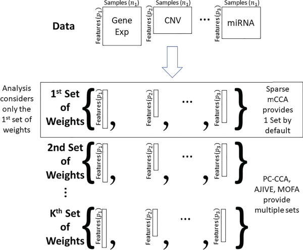
Each method shown in the figure generates a set of weights for each data type. Our analysis only considers the first set of weights to avoid issues related to a potentially complex set of mappings of factors across data splits.

Once contributions are found for each data type, they can be plotted against the contributions of another data type to visualize the relationships identified by the multi-omics method of interest. Additionally, samples that fall off of the diagonal in a contribution plot may be biologically meaningful outliers, or technical outliers for one of the assays. This plot is termed the ‘contribution plot’, and we can identify method overfitting using a cross-validation analysis.

Cross-validation

The unsupervised nature of the multi-omics methods makes it difficult to determine whether a method is overfitting or identifying a true biological relationship. Data splitting and the projection of estimated contributions were proposed by Soneson et al. (2010) [11] for parameter tuning and validation of a multi-omics method. Other methods have assessed method performance by using leave-one-out cross-validation and the projection of learned factors on new datasets [12]; [13]. By omitting a subset of the samples from the analysis and predicting their contributions from each data type in the training set, we can discern whether the relationships from the full analysis suffer from overfitting or provide unstable results. Our analysis pipeline is shown in Figure 2. We chose to divide the data into training and test sets of approximately 80% / 20% of the total samples. Using the 80% training set, analyses were done for each method, and corresponding weights were generated for each data type. Contributions were calculated for the test set by multiplying the weights derived from the training set by the test set data in the manner appropriate to each method, as defined above. Critically, our cross-validation loop used for evaluation of methods takes place ‘outside’ of any permutation or cross-validation that a method may use during training or fitting of its model parameters, such as the calculation of feature weights for each data type.

Figure 2.

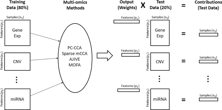
Pipeline for cross-validation analysis. Training data: Dataset is subset to 80% of the original data and will be used to train the model. Multi-omics methods: The training data are analyzed using the specified method. Output: Weights are output from the multi-omics methods. Test data: The remaining 20% of the original data are used as test data and multiplied by the subsequent weights. Contributions: The result of multiplying the output weights by the test set data. Each sample in the test data yields one number that represents the contribution per data type.

The results of the methods may not be unique, which can lead to slight alterations in scaling and sign. Due to this, the results across folds may identify the same biological process, but provide results of different magnitudes. To account for this, we scale and change the sign of the cross-validated contributions to ensure that they are positively correlated with the results from the full analysis. This procedure is performed separately for each fold. The sign is flipped if the correlation between the cross-validated and full-analysis contributions is negative, while scaling is achieved by subtracting the mean and dividing it by either the standard deviation or the median absolute deviation. If the contributions are not unimodal or contain outliers, we recommend using the median absolute deviation for scaling.

To avoid difficulties in aligning weights across folds, in our evaluation we only consider the set of weights corresponding to the first factor. In MOFA, factors are arbitrarily labeled and thus no formal ordering is defined for the ‘first’ or ‘second’ factor. Repeating the analysis will yield a different labeling scheme for each factor while factors are still describing the same biological process. This necessitates the alignment of factors across multiple folds and creates a computational challenge. For sparse mCCA and MOFA, the first set of weights or first factor typically yields the strongest pair-wise correlations. As more sets of weights are estimated, the correlations typically decrease (see Figure 2B in [6]). Lower factors may be more susceptible to fluctuations, such as sampling variability in the samples chosen for the training set.

After the contributions are appropriately scaled, contribution plots can be constructed for each pair-wise combination of the assays in the test set. We will refer to these plots as the cross-validation (CV) contribution plots and the contribution plots from the full analysis as the full contribution plots. By examining the change in correlations between the CV contribution plots and the full contribution plots for each pair-wise data type pair, we may observe the degree to which each method suffers from overfitting. The full contribution plots reflect the typical results that a user would observe when running a method on their entire dataset, while the CV contribution plots reveal any issues with the generalization of feature weights for new data, in that we observe the correlations obtained on all samples in the dataset when those samples are not used for training. It is important to note that because the identified factor may only be a small portion of the entire solution, the correlation of the contribution plot should not be compared across methods, but rather within one method by comparing the correlation in the full analysis to the correlation in the cross-validated analysis. Methods like AJIVE and MOFA identify a multi-dimensional solution, and thus, a low correlation in the contribution plot may not indicate that the method is performing poorly, but rather that the top factor captures a low correlation between the two data types of interest. Figure 3 provides examples of good and poor results for the contribution plot generated using artificial data. Figure 3A shows a strong correlation in both the full and CV contribution plots, indicating that the method is not overfitting and that the two data types are related. Figure 3B shows no correlation in the full and CV contribution plots, which also indicates that the method is not overfitting, but rather, that the two data types are not related. Figure 3C shows a strong correlation in the full contribution plot and no correlation in the CV contribution plot, thus demonstrating that the method is overfitting on the data and that there does not appear to be a relationship between these two data types. We also generate ‘overfitting plots’, which plot lines connecting the pair-wise correlations of the full and cross-validated contribution plots to provide a useful overview of the change in correlation between the full and CV analysis for all pairs of assays. We also plot contributions from the cross-validation analysis against contributions from the full analysis within each data type. We call these the ‘comparison plots’, and a strong linear correlation indicates method consistency.

Figure 3.

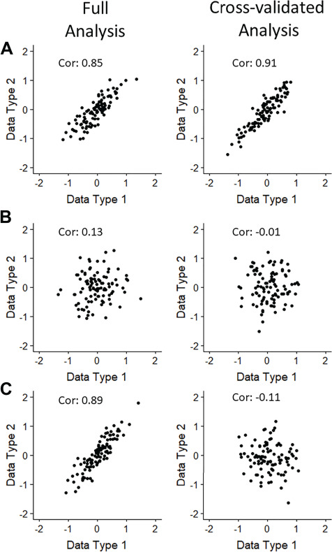
The figure provides hypothetical scenarios for the contribution plot, generated using artificial data. A. A strong correlation in both the full and CV plots, indicating that the method accurately fits the data and that the two data types are linearly related. B. A null correlation in both the full and CV plots, indicating that the method did not overfit and that the two data types are not related in terms of this factor. C. A strong linear relationship in the full plot and a null relationship in the CV plots, indicating that the method overfit and that the two data types are not associated with the top factor.

Multi-omics datasets

Data from The Cancer Genome Atlas (TCGA) [3] [14] was used to evaluate method performance for sparse mCCA, AJIVE and MOFA. We applied these three methods to 558 breast cancer samples using copy number variation (CNV), RNA expression and micro RNA expression. CNV was summarized for 216 segments; RNA expression was measured for 12 434 genes; and miRNA expression was measured for 305 miRNAs. Five folds were selected for the analysis, and fold membership was fully randomized. Contribution and comparison plots were generated for each data type to evaluate the degree of overfitting and the consistency of the results.

Data from Li et al. (2016) [15] were used as a second validation dataset. This collection of datasets contained fewer samples and thus was used to examine stability of methods with smaller sample sizes. RNA expression, DNase and protein expression were collected for lymphoblastoid cell lines from Yoruban individuals. DNase was measured for 699 906 peaks; RNA expression was measured for 13 967 genes; and protein expression was measured for 4375 proteins for 53 samples.

To demonstrate the ability of our framework to identify overfitting, we analyzed datasets with no relationship across assays, referred to as null datasets, using PC-CCA, sparse mCCA, AJIVE and MOFA. Permuted null datasets were generated by permuting the samples for each data type in the TCGA breast cancer data. Because PC-CCA can only accommodate two data types, we used only RNA and miRNA for this analysis. Five folds were selected for the analysis, with the fold membership being fully randomized. For all datasets, contribution plots, comparison plots and overfitting plots were generated to evaluate method performance.

Evaluation of methods

We applied our evaluation framework to datasets with both large (TCGA breast cancer) and small (Li et al.) sample sizes, as well as a permuted null dataset. Sparse mCCA, AJIVE and MOFA all demonstrate consistency and a lack of overfitting in the large-sample size analysis. The overfitting plots for the large-sample size analysis (Figure 4A–C) have near zero slopes, indicating that the relationships found in the training set generalize to the held out set. The difference in the magnitude of the correlations across methods does not indicate a lack of overfitting, but rather that the top factor indicated a strong or weak relationship between the specified data types. This artifact is not necessarily a limitation of the method, but rather might be explained by the fact that we are considering only the first set of weights in our analysis. Side-by-side contribution plots (Supplementary Figures 2–10) also demonstrate a lack of overfitting and confirm that there are no sample outliers that are overly influencing the results. Comparison plots (Supplementary Figures 11–13) show that the contributions for the CV analysis and full analysis are similar, indicating overall method consistency. AJIVE was observed to have reduced pair-wise correlations for contributions including the CNV assay, and this result persisted after attempting with a higher pre-specified rank (Supplementary Figure 14). Overall, for the large-sample size analysis, we found that sparse mCCA and MOFA did not overfit and found large pair-wise correlations between contributions from all assays. AJIVE also showed a lack of overfitting; however, a large pair-wise correlation was only found between RNA and miRNA.

Figure 4.

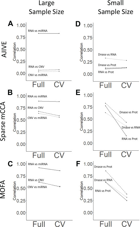
Overfitting plot: Plots of the pair-wise correlations identified in the full and CV contribution plots for each method. The left column (plots A–C) corresponds to the large-sample analysis (n = 558; TCGA breast cancer), while the right column (plots D–F) corresponds to the small-sample size analysis (n = 53; Li, et al. 2016). Rows correspond to AJIVE, sparse mCCA and MOFA, respectively. Flat lines indicate non-overfitting methods, while lines with a negative slope indicate a large change in the results for the full and CV plots.

We further investigated the contributions for AJIVE, sparse mCCA and MOFA. Contributions from Sparse mCCA are highly correlated (, Pearson correlation coefficient) with MOFA across all data types. AJIVE contributions have strong negative correlations with both Sparse mCCA () and MOFA () for mRNA (noting that the sign here is arbitrary), while exhibiting a moderate negative correlation in miRNA (. AJIVE contributions for CNV are not correlated with Sparse mCCA () or MOFA () (Supplementary Figures 15–17). mRNA contributions for all methods were found to be bimodal and highly correlated with the expression of the estrogen receptor 1 (ESR1) gene (Supplementary Figure 18). Previous studies have found that the expression of the ESR1 gene is amplified in a subset of breast cancers, providing some biological validation for the top contribution—estimated without any prior information about ESR1 gene expression—for all methods run on this dataset [16].

Alternatively, in the small-sample size analysis, sparse mCCA and MOFA appear to overfit in the full analysis, while AJIVE does not overfit. Plot 4D shows a lack of overfitting with AJIVE in the small-sample analysis, while plots 4E and 4F show a consistent drop in the correlation for the CV analysis. Thus, sparse mCCA and MOFA are able to identify strong linear relationships in the full analysis, but the correlations are substantially reduced in the CV analysis. This may reflect a reduced ability for consistent detection of top factors for small-sample datasets. Side-by-side contribution plots (Supplementary Figures 19–27) show more clearly a decrease in correlation with sparse mCCA and MOFA, but not with AJIVE, which maintains a relatively weak correlation in both analyses. Comparison plots (Supplementary Figures 28–30) show less consistency than in the large-sample analysis.

We assessed the degree to which the results were robust when varying the number of folds. Sparse mCCA was used to analyze the small-sample size dataset using both 3- and 10-folds. The 3-fold analysis yielded small training set sizes, which led to poor prediction for the test set samples (Supplementary Figure 31). Alternatively, in the 10-fold analysis, small test set sizes made contribution scaling difficult, which also led to reduced correlation of the cross-validated contributions with the full set contributions (Supplementary Figure 32). Additionally, many methods have extensive run times and thus conducting an analysis with many folds can create a prohibitive computational burden.

Analyses for the permuted null dataset showed that PC-CCA using 100 PCs per data type identifies a strong relationship between miRNA and RNA when no relationship exists (Figure 5A). Sparse mCCA correctly identifies no relationship (Figure 5B) in the full analysis; AJIVE and MOFA also identify no relationship (Supplementary Figures 33–34). These plots show the ability of our framework to identify overfitting, as well as the ability of sparse mCCA, AJIVE and MOFA to not overfit the null dataset.

Figure 5.

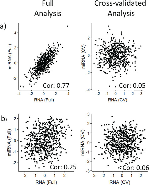
Side-By-Side contribution plots for a) PC-CCA with 100 PCs and b) Sparse mCCA with the null dataset: Left panels show the contribution plots from the full analysis, while right panels show the contribution plots for the CV analysis. Pair-wise correlations are reported on the figure.

Discussion

In this paper, we have proposed a framework and approach for the evaluation of unsupervised multi-omics methods. Sparse mCCA, AJIVE, MOFA and PC-CCA were compared based on consistency and the degree of overfitting in one large-sample size dataset, one small-sample size dataset and one permuted null dataset. All methods performed well with the large-sample dataset, with AJIVE somewhat underperforming by failing to detect a contribution from CNV to the top factor, which other methods detected and which had stable correlation in cross-validated contributions. However, both sparse mCCA and MOFA showed some evidence of either overfitting or lack of consistency with the small-sample dataset. PC-CCA overfit the null dataset, while the other methods accurately identified a null relationship. Previous work [9] looked at the sensitivity and specificity of methods using simulated data. In contrast, our framework examines the extent of overfitting and does not make any simulation assumptions.

There are now dozens of methods for unsupervised multi-omics data analysis, and the list continues to grow. Other multi-omics approaches that we did not compare here use re-formulations of partial least squares [17], or co-inertia analysis [18], and often make use of a lasso penalty or sparse thresholding to induce sparsity on feature weights [19].

Future work may include investigation into the alignment of weights across folds and replications and how to incorporate more than one set of weights. Argelaguet et al. (2019) [20] propose comparing the Pearson correlation coefficient between every pair of factors as a way to address these concerns. Additionally, classical CCA could be used to perform matching of factors across folds or replicate runs, by running CCA on every pair of contributions. We did not evaluate the sensitivity and specificity of the methods we tested, as they are designed to describe variation, rather than classification, of samples. A separate analysis similar to Pucher et al. (2018) [9] would be needed to evaluate AJIVE and MOFA on the claims of accuracy. Here we examined the biological meaningfulness of the top factor found in the TCGA breast cancer dataset by plotting the mRNA contributions against expression of estrogen receptor 1, for which we have, from literature, some external support of its relevance as a primary axis of co-variation of molecular profiles of breast tumors. In general, downstream assessment of the biological meaningfulness of a factor can be achieved through gene set analysis, by defining the observed gene set as the non-zero or top weighted genes from the gene expression weights estimated by the multi-omics methods. The MOFA R package includes a function for performing this type of ‘Feature Set Enrichment Analysis’. For non-gene expression features, non-zero or top weights for features can be examined with respect to their co-localization with weights from other data types on the genome, or with various publicly available genomic tracks such as cell-type specific regulatory regions [21][22].

We provide an R package called MOVIE (Multi-Omics VIsualization of Estimated contributions) and documentation to assist with the comparison of future methods and datasets using our framework. Package source code is publicly available: https://github.com/mccabes292/movie.

Key Points

• Cross-validation provides a useful framework for evaluating unsupervised multi-omics methods in which the true common variation across biological modalities is not known.

• Sample sizes of n = 50 or below may result in inconsistent fitting of multi-omics methods, where correlations found in training data do not generalize to held out data.

• The contribution plot, where contributions to the common variation space from two modalities are plotted against each other, provides a useful visual summary of the result of multi-omics methods.

Sean D. McCabe is a PhD student in the Department of Biostatistics at the University of North Carolina at Chapel Hill.

Dan-Yu Lin is the Dennis Gillings Distinguished Professor in the Department of Biostatistics at the University of North Carolina at Chapel Hill.

Michael I. Love is an assistant professor in the Department of Biostatistics and the Department of Genetics at the University of North Carolina at Chapel Hill.

Funding

The work of S.D.M. was supported by a National Institutes of Health grant [T32 CA106209-12]. The work of D.Y.L. was supported by National Institutes of Health grants [P01 CA142538, R01 HG009974]. The work of M.I.L. was supported by National Institutes of Health grants [R01 HG009125, P01 CA142538, P30 ES010126].

References

- 1. Shen R, Olshen AB, Ladanyi M. Integrative clustering of multiple genomic data types using a joint latent variable model with application to breast and lung cancer subtype analysis. Bioinformatics 2010;26(2):292–3, doi: 10.1093/bioinformatics/btp659. [DOI] [PMC free article] [PubMed] [Google Scholar]
- 2. Wang B, Mezlini AM, Demir F, et al. Similarity network fusion for aggregating data types on a genomic scale. Nat Methods 2014;11:333–7 doi: 10.1038/nmeth.2810, 3, PMID:24464287. [DOI] [PubMed] [Google Scholar]
- 3. Wong KY, Fan C, Tanioka M, et al. I-boost: an integrative boosting approach for predicting survival time with multiple genomics platforms. Genome Biol 2019;20:52,1, doi: 10.1186/s13059-019-1640-4, PMID:30845957. [DOI] [PMC free article] [PubMed] [Google Scholar]
- 4. Witten DM, Tibshirani RJ. Extensions of sparse canonical correlation analysis with applications to genomic data. Stat Appl Genet Mol Biol 2009;8(1):28. [DOI] [PMC free article] [PubMed] [Google Scholar]
- 5. Feng Q, Jiang M, Hannig J, et al. Angle-based joint and individual variation explained. Journal of Multivariate Analysis 2018;166,241–265. [Google Scholar]
- 6. Argelaguet R, Velten B, Arnol D, et al. Multi-Omics factor analysis—a framework for unsupervised integration of multi-omics data sets. Mol Syst Biol 2017;14:e8124. [DOI] [PMC free article] [PubMed] [Google Scholar]
- 7. Hotelling H. Relations between two sets of variates. Biometrika 1936;28,321–77, 3-4, doi: 10.1093/biomet/28.3-4.321. [DOI] [Google Scholar]
- 8. Meng C, Zeleznik OA, Thallinger GG, et al. Dimension reduction techniques for the integrative analysis of multi-omics data. Brief Bioinform 2016;17(4),628–41, doi: 10.1093/bib/bbv108. [DOI] [PMC free article] [PubMed] [Google Scholar]
- 9. Pucher BM, Zeleznik OA, Thallinger GG. Comparison and evaluation of integrative methods for the analysis of multilevel omics data: a study based on simulated and experimental cancer data. Brief Bioinform 2019;20(2),671–681, 10.1093/bib/bby027. [DOI] [PubMed] [Google Scholar]
- 10. Tini G, Marchetti L, Priami C, et al. Multi-omics integration—a comparison of unsupervised clustering methodologies. Brief Bioinform, bbx167, 10.1093/bib/bbx167. [DOI] [PubMed]
- 11. Soneson C, Lilljebjörn H, Fioretos T, Fontes M. Integrative analysis of gene expression and copy number alterations using canonical correlation analysis. BMC Bioinformatics 2010;11,191, 1, doi: 10.1186/1471-2105-11-191. [DOI] [PMC free article] [PubMed] [Google Scholar]
- 12. Brown BC, Bray NL, and Pachter L Expression reflects population structure. PLOS Genetics 2018;14(12), e1007841 10.1371/journal.pgen.1007841. [DOI] [PMC free article] [PubMed] [Google Scholar]
- 13. Fertig EJ, Ren Q, Cheng H, et al. Gene expression signatures modulated by epidermal growth factor receptor activation and their relationship to cetuximab resistance in head and neck squamous cell carcinoma. BMC Genomics 2012;13,160, 1, doi: 10.1186/1471-2164-13-160. [DOI] [PMC free article] [PubMed] [Google Scholar]
- 14. Broad Institute TCGA Genome Data Analysis Center Analysis-ready standardized TCGA data from Broad GDAC Firehose 2016_01_28 run.
- 15. Li YI, van de Geinj B, Raj A, et al. RNA splicing is a primary link between genetic variation and disease. Science 2016;352(6285):600–4, doi: 10.1126/science.aad9417. [DOI] [PMC free article] [PubMed] [Google Scholar]
- 16. Holst F, Stahl PR, Ruiz C, et al. Estrogen receptor alpha (ESR1) gene amplification is frequent in breast cancer. Nat Genet 2007;39,655–60, 5, doi: 10.1038/ng2006. [DOI] [PubMed] [Google Scholar]
- 17. Lê Cao KA, Martin PGP, Robert-Granié C, Besse P. Sparse canonical methods for biological data integration: application to a cross-platform study. BMC Bioinformatics 2009;10:34, 1, doi: 10.1186/1471-2105-10-34. [DOI] [PMC free article] [PubMed] [Google Scholar]
- 18. Meng C, Kuster B, Culhane AC, Gholami A. A multivariate approach to the integration of multi-omics datasets. BMC Bioinformatics 2014;15:162, 1, doi: 10.1186/1471-2105-15-162, PMID:24884486. [DOI] [PMC free article] [PubMed] [Google Scholar]
- 19. Rohart F, Gautier B, Sing A, et al. mixOmics: an R package for’omics feature selection and multiple data integration. PLoS Comput Biol 2017;13(11). [DOI] [PMC free article] [PubMed] [Google Scholar]
- 20. Argelaguet R, Mohammed H, Clark S, et al. (2018). Single cell multi-omics profiling reveals a hierarchical epigenetic landscape during mammalian germ layer specification. bioRxiv, 519207; doi: 10.1101/519207. [DOI] [Google Scholar]
- 21. ENCODE Project Consortium (2012). An integrated encyclopedia of DNA elements in the human genome. Nature, 489(7414):57–74, doi: 10.1038/nature11247, PMID:22955616. [DOI] [PMC free article] [PubMed] [Google Scholar]
- 22. Roadmap Epigenomics Consortium Integrative analysis of 111 reference human epigenomes. Nature 2015;518:317–30. [DOI] [PMC free article] [PubMed] [Google Scholar]
Associated Data
This section collects any data citations, data availability statements, or supplementary materials included in this article.