

Abstract
Studying sets of genomic features is increasingly popular in genomics, proteomics and metabolomics since analyzing at set level not only creates a natural connection to biological knowledge but also offers more statistical power. Currently, there are two gene-set testing approaches, self-contained and competitive, both of which have their advantages and disadvantages, but neither offers the final solution. We introduce simultaneous enrichment analysis (SEA), a new approach for analysis of feature sets in genomics and other omics based on a new unified null hypothesis, which includes the self-contained and competitive null hypotheses as special cases. We employ closed testing using Simes tests to test this new hypothesis. For every feature set, the proportion of active features is estimated, and a confidence bound is provided. Also, for every unified null hypotheses, a  -value is calculated, which is adjusted for family-wise error rate. SEA does not need to assume that the features are independent. Moreover, users are allowed to choose the feature set(s) of interest after observing the data. We develop a novel pipeline and apply it on RNA-seq data of dystrophin-deficient mdx mice, showcasing the flexibility of the method. Finally, the power properties of the method are evaluated through simulation studies.
Keywords: pathway analysis, multiple pathways, GWAS, closed testing, self-contained approach, competitive approach
Introduction
In a typical genomics study, one would measure over a thousand features, e.g. DNA sequence, structural variation or gene expression. The goal is to detect features that are active (e.g. differentially expressed) under a certain phenotype condition. Traditionally, association of each feature with the phenotype is tested, and using multiple testing procedures, a long list of  -values with a controlled error rate is created. A well-established alternative is to define sets as groups of homogeneous features (e.g. similar function or location) and test their association with the phenotype [1]. Testing feature sets rather than individual features allows more direct interpretation of the underlying biological processes as well as giving more power to detect subtle effects.
If many feature sets are tested, multiple testing correction must be used. Controlling false discovery rate (FDR) is common for genomics studies; however, some authors have argued that control of family-wise error rate (FWER) is more appropriate when testing feature sets [2–4]. Feature sets of interest are generally determined based on one or many feature-set collections, for example Gene Ontology (GO) [5], Kyoto Encyclopedia of Genes and Genomes (KEGG) [6], Molecular Signatures Database [7], Panther Database [8], WikiPathways [9] etc. Since the choice of database can greatly affect the analysis result, it is very tempting to use several databases. However, current multiple testing methods require that the feature sets are chosen independent from the data at hand. Using many databases simultaneously results in a severe multiple testing correction.
There are many options to test for association of a given feature set with phenotype [10, 11]. Broadly, we can distinguish two types of approaches by their choice of null hypothesis [12]. Methods testing the competitive null test whether features in the feature set of interest are more often active than features outside the feature set. Methods testing the self-contained null test whether there are any active features in the feature set of interest. Examples of competitive methods are Fisher’s exact test [13], Gene Set Analysis (GSA) [14], Significance Analysis of Function and Expression (SAFE) [15] and Gene Set Enrichment Analysis (GSEA) [1]. Self-contained methods include global test [16], GlobalANCOVA [17] and FORGE [18].
The two approaches may produce widely different results [19], and there is an ongoing debate over the suitability of self-contained versus competitive methods. Self-contained methods are criticized for ignoring the information in the complement of the feature set: detecting at least one active feature in the feature set is not very informative if the complement of the feature set has more active features than the set itself [20, 21]. Competitive methods have been criticized for relying on an unrealistic assumption of independence of features [22, 23]. Moreover, the competitive null hypothesis is not always statistically as well defined. Wu [22] suggest that competitive tests are still used despite their methodological drawbacks because there are no statistically sound alternative methods that would ‘maintain the direct interpretation of competitive tests’. Attempts have been made to avoid the assumption of independence of features in competitive methods by a permutation approach. However, Maciejewski [24] convincingly argued that in general the resulting methods do not in fact test the competitive but the self-contained null. Only in the case of GSEA, did Debrabant [25] show under restrictive assumptions that the permutation version of GSEA tests the competitive null. So far, there is no general method that tests the competitive null hypotheses and is valid under dependence of features.
This article proposes a novel approach unifying competitive and self-contained testing into a single framework. We introduce a general null hypothesis, related to the partial conjunction hypothesis [26], that asserts that the proportion of truly active features is less than some threshold. By varying the threshold, the self-contained and competitive null hypotheses are included as special cases. We embed this general null hypothesis in a multiple testing framework that controls FWER for all unified null hypotheses for all thresholds simultaneously. Remarkably, therefore the framework also includes all competitive and self-contained null hypotheses of all possible feature sets, i.e. all subsets of the total set of features. Consequently, the choice for testing a competitive or self-contained null hypothesis may even be postponed until after seeing the data. Since FWER is controlled over all possible feature sets, even the database of feature sets may be chosen after seeing the data without compromising type I error control. The method gives FWER-adjusted  -values for the null hypotheses for any set of interest for any threshold. More importantly, it also gives a simultaneous confidence interval for the proportion of active features in the set.
Our approach is based on the All-Resolutions Inference (ARI) of Goeman and Solari [27] and Goeman et al. [28], which uses a combination of closed testing [29] and the Simes test [30]. A similar approach has recently been advocated for testing brain regions in neuroimaging [31]. This approach is valid under certain forms of dependence between features, as long as the Simes inequality can be assumed to hold for the set of all non-active features. This is the same assumption required for the validity of FDR control by the widely accepted method of Benjamini and Hochberg (BH) [32].
The paper is organized as follows: first, we present a brief review of the properties of self-contained and competitive tests. Next we introduce the unified null hypothesis and show that it encompasses both earlier definitions. Then we briefly revisit the ARI and adapt it to test the unified null. We apply simultaneous enrichment analysis (SEA) to an RNA-seq data set and suggest a general pipeline for testing sets of genomic features. Finally, we study the power of the new method in comparison to previous approaches by a simulation experiment.
Self-contained versus competitive methods
Various statistical methods have been established for feature-set testing since its inception, and many studies have compared them in terms of power, false positive rate, sensitivity and reproducibility, for a recent review refer to [33]. As mentioned above, these methods are broadly categorized as self-contained or competitive. In this section, we briefly review the advantages and disadvantages of each category.
Self-contained methods aim to test  : ‘None of the features in the set are active’ [12]. This is a very classical type of null hypotheses in statistics (familiar from e.g. ANOVA models). Therefore, self-contained tests are typically based on classical and sound statistical models that have the subject as the sampling unit. Consequently, whether based on subject permutation or on parametric methods, correlations between features are correctly taken into account. Self-contained methods are statistically well founded: this is the main selling point of these methods. As a consequence, self-contained methods have been found to be highly reproducible: there is a high chance of achieving similar results with a new set of subjects [33]. Moreover, self-contained tests are powerful for feature sets of all sizes and can even be meaningfully applied to the feature set of all features and to singleton feature sets [12].
However, self-contained tests have been criticized for being too powerful. This is because the null hypothesis is too specific: it is false even if a single active feature is present in a set of many features. If many features in the data are active, then the self-contained null hypotheses will generally be false for almost all feature sets, especially for large ones. This means that self-contained methods can be less specific in distinguishing feature sets that are associated with e.g. polygenic phenotypes [20].
Competitive methods aim to test  : ‘Features in the set are at most as active as the background features’. The background (or reference) features are all the features that are not in the feature set of interest. Feature sets for which the competitive null hypothesis is not true are called enriched with active features. Competitive hypotheses are more specific because they look for feature sets that stand out in comparison with other feature sets. This way, competitive tests correct for the biological processes in the background. It has been claimed that not only the undesired and shared biological effects but also genome-wide confounding effects are excluded [20]. Thereby, the approach adds biological relevance to the analysis. This is the main reason for using competitive methods. It is especially relevant if there are many active features in the data set. Obviously, the background should be chosen with care to ensure proper biological interpretation, and any feature filtering steps should be properly taken into account [34–36].
Most competitive tests rely on the crucial assumption that features are independent, either explicitly or because they calculate  -values by feature permutation [24]. An advantage of this assumption is that the methods can be used even for a study with only two biological samples [37, 38]. However, the assumption of independent features is almost always highly unrealistic. If this assumption is violated, the results of competitive methods cannot be trusted. Even in the presence of small correlations between features competitive methods have excessive type I errors, as has been demonstrated by many authors [14, 22, 23, 35,
39–41].
-values by feature permutation [24]. An advantage of this assumption is that the methods can be used even for a study with only two biological samples [37, 38]. However, the assumption of independent features is almost always highly unrealistic. If this assumption is violated, the results of competitive methods cannot be trusted. Even in the presence of small correlations between features competitive methods have excessive type I errors, as has been demonstrated by many authors [14, 22, 23, 35,
39–41].
Some competitive methods, such as SAFE, GSA and GSEA, avoid the problematic independence assumption by switching to subject permutation to calculate  -values. Such hybrid methods [12] indeed have lower false-positive rates than other competitive methods [41]. Critically, Maciejewski [24] showed that GSEA and SAFE do not actually test the competitive null hypothesis, which makes the results difficult to interpret. In fact, the null hypothesis of such hybrid methods is false if any feature either in or out of the set is active. This means that hybrid methods do not in general provide valid statistical tests for the competitive null hypothesis. Only for the case of GSEA and under strong assumptions, did Debrabant [25] suggest that the method truly tests the competitive null hypothesis.
Both approaches have their advantages and disadvantages. Self-contained methods are statistically well founded but may not always test the biologically relevant null hypothesis. Competitive methods do test the biologically relevant null hypothesis, but all available methods rely on strong or unrealistic assumptions.
The unified null hypothesis
We now unify the self-contained and competitive methods into a single null hypothesis  , that contains both types of null hypothesis as special cases.
Suppose that a genomics experiment is performed with  features. Denote the set of all features by
  . An unknown subset
  of these are truly active (A). We are interested in testing feature-set
  . We denote the number of truly active features in
  as
as  where
where  refers to the size of set. Define
  , the proportion of active features in
  . The competitive and self-contained null hypotheses can now both be formulated in terms of
  .
.
By the definition from [12], the self-contained null hypothesis says that the proportion of active features is zero, so it is defined as
 |
Similarly, the competitive null hypothesis says that the proportion of active features in  is at most equal to the proportion in the background. The background is the complement of the set
  , denoted by
  . The competitive null is therefore defined as
As we show in Methods,  is logically equivalent to
 |
To understand this, assume that the feature-set  has a smaller proportion of active features than its complement
  , then it must also have a smaller proportion of active features than the set of all features
  . Conversely, if the set has a smaller proportion than the set of all features, this must be because the complement has a larger proportion than the set itself. A formal proof is provided in the supplementary material.
We see that both hypotheses are special cases of the unified hypothesis
 |
for  . By varying
  , we may obtain the competitive test by taking
  or the self-contained test by taking
  . However, we may also take other values of
  . By testing the unified null hypothesis for all values of
  , we automatically test both the self-contained and the competitive null hypotheses. We note that
  is always a multiple of
  , so only values of
  that are a multiple of
  make sense to test.
All-resolutions inference
In practical applications, we are not interested in making inferences about a single feature set but about multiple feature sets. Moreover, we are not necessarily interested in a single value of  . The ARI approach [27, 28,
31] allows testing the unified null hypothesis for all
. The ARI approach [27, 28,
31] allows testing the unified null hypothesis for all  and all
  , while controlling the FWER at level
  . This means that with probability at least
  no type I error is made, where a type I error is defined as rejection of any true unified null hypothesis
  for any
  . This is a huge multiple testing burden, involving
  sets
sets  and many values
  for every
  . This burden is surmounted by ARI using the closed testing procedure [29], which exploits the overlaps between the various sets
  to great effect. Technical details are given in the Methods section and in [27] and [28].
Control of FWER for all  and
and  allows the user to postpone the choice of
  and
and  until after seeing the data without incurring additional type I errors due to this data peeking. Thereby, we do not need to choose feature sets from a single feature-set database but allow ourselves to combine many such databases. A feature set may even be chosen on the basis of the data without reference to any database. By testing all values of
  simultaneously, we will be testing both the self-contained and the competitive null hypotheses for all feature sets. If multiple
  and
and  are chosen, the final results have automatic FWER control. This FWER control also encompasses the individual features, i.e. singleton feature sets.
For every feature-set  , ARI produces an estimate
  and a 95% confidence bound
  for the proportion of active features in
  . These have the properties that
  simultaneously for all
  with probability at least 50% and that
  simultaneously for all
  with probability at least 95%. The simultaneous confidence interval for
  is therefore
  . It always contains the estimate
  but is not necessarily centered on it. The confidence intervals are necessarily one sided: it is impossible to prove that features are non-active since we cannot prove a null hypothesis.
Based on this confidence interval, ARI rejects  if and only if
  . A FWER-adjusted
  -value can be calculated for every
  , as we show in the Methods section. It is defined as the smallest
  -level that allows rejection of
  within the ARI framework. Consequently, this
  -value is smaller than 5% if and only if
  . By testing all
  for all
  , we automatically test the competitive null hypothesis for all
  . However, the definition uses
  , which is not known. Practically, we may plug in an estimator of
  . It should be remarked that the FWER control is guaranteed for the unified null at the plugged-in threshold. Control at the real value of
  is only guaranteed if correlations between features are low, as explained in the Methods section.
ARI is not assumption free. It requires that the Simes inequality [30] holds for the subset  of truly inactive features. It has been shown to hold whenever the
  -values are independent or positively correlated [42]. The assumption needed for ARI is needed for the validity of BH [32] as an FDR-controlling procedure. It is a much less restrictive assumption than the independence assumption that is invariably made by competitive methods.
Methods
In this section, we present details on the ARI method of Goeman and Solari [27] and its use to test the unified null hypothesis simultaneously for all feature sets. Within this framework, we create a closed testing procedure for all self-contained null hypotheses first. From this, we derive simultaneous confidence intervals for the proportion of active features in all feature sets, which are in turn used to test the unified null hypothesis.
Simes tests
We will first construct a multiple testing procedure for all  self-contained null hypotheses and then explain how the same procedure can actually be used to test all unified null hypotheses. To test the self-contained null hypothesis of a set
  , we use the Simes test. This test rejects the self-contained null hypothesis at level
  if and only if
  , where
 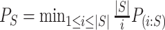 and
and  stands for the ith ordered
  -value among features in
  .
.
The Simes test is valid under quite general dependency structures between the  -values, including independence but not when too many negative correlations between
  -values occur [42, 44–46]. The conditions under which the Simes test controls type I error are weaker than those required by the FDR controlling procedure of BH [32], to which it is closely related. The BH procedure requires the
  -values to satisfy the ‘positive regression dependence on a subset (PRDS)’ property, which is generally assumed to hold for genomics data [43]. For the Simes test, the ‘positive regression dependence within nulls (PRDN)’ is sufficient, which is a weaker assumption than PRDS [47].
Closed testing
To control FWER over the self-contained null hypotheses for all subsets, we use the closed testing procedure. In closed testing, the hypothesis for a set  is rejected if and only if the hypotheses for all supersets of
  , including
  itself, have also been rejected. Closed testing guarantees that FWER is controlled for all hypotheses for all
  sets
sets  .
.
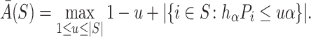
In general, closed testing procedures have an exponential computational load, but for the case of closed testing with Simes tests, the computations can be done much more efficiently. As shown by [28],  is rejected if and only if for some
  , we have
 |
(1) |
where
 |
(2) |
The dependence of  on
on  is made explicit by its subscript. Note that
  does not depend on
  .
.  can be interpreted as the size of largest feature-set
  for which
  is not rejected at level
  . We also have that
  . Meijer et al. [48] introduced an algorithm to calculate
  for all values of
  simultaneously in linearithmic time. After
  has been found, deciding whether
  is rejected takes only linear time in
  for each
  .
.
Estimates and confidence intervals
It was shown by [27] that any closed testing procedure can be used to make simultaneous confidence intervals for  . The reasoning is briefly as follows: suppose that all subsets of
  of size
  have been rejected by the closed testing procedure. If the closed testing procedure did not make a type I error, then every subset of
  of size
  must contain at least one active feature. Consequently,
  must contain at least
  active features. Since the probability that the closed testing procedure makes no error is at least
  , we have
  . For every
  , we find the smallest value of
  , say
, say  , such that all
  -sized subsets of
  have been rejected by the closed testing procedure. Then
  . Importantly, since the event that the confidence interval does not cover
  is the event that the closed testing procedure makes an error, which is the same for every
  , the confidence intervals are automatically simultaneous. We have
 |
(3) |
The simultaneity in (3) means that the true values of  for all
  are all within these bounds with probability at least
  . This implies that also any selected
  is within the bounds. Simultaneity of confidence bounds makes them robust against selection.
In general, calculation time of  is exponential. For the case of Simes tests, however, calculations simplify. Goeman et al. [28] showed that
  , where
 |
Taking  , we obtain the confidence lower bound, leading to the confidence interval
  . Taking
  , we obtain the point estimate
  . The probability of the true proportion
  of active features exceeding the estimate is at most 0.5 (the estimate is ‘median unbiased’). More liberal than the confidence bound, this estimate is useful to get a conservative impression of the likely amount of activation in the selected set
  . Since the 50% confidence intervals that give rise to the point estimate are still simultaneous, this estimate retains its property of median unbiasedness even over selected
  .
.
Testing unified null hypotheses
Clearly, (1) tests  for
for  for all
  since this is the self-contained null hypothesis. To test the unified null hypothesis, we reject if and only if
  . To see that this is a valid test, let
  be true, so that
  . Then we have
  . Simultaneity over all
  and all
  , and consequently FWER control, follows immediately from the simultaneity of the confidence bounds. If the closed testing procedure did not make an error, which happens with probability at least
  , no unified null hypothesis, for any
  or any
  , is falsely rejected.
For closed testing with Simes tests, we reject  if and only if there is an
  such that
 |
(4) |
where  .
.
To test the competitive null hypothesis, we should use the unified null hypothesis with  . However, usually
  is unknown, and we need to replace it with an estimate
  . Then, we reject the competitive null hypothesis for
  if
if  .
.
To keep type I error control, it is important that  underestimates
  at most as much as
  underestimates
  . Goeman et al. [28] showed that the bounds
  are more conservative for small sets
  than for larger sets. Consequently, we know that on average
  underestimates
  less than
  underestimates
  . Therefore, we propose to use
  .
.
Like above for the unified test, we use a constant  that is an integer multiple of
  . However, instead of rounding down as we could with a fixed
  in the unified test, we now round up in order to conserve the necessary property that
  does not underestimate
  too much. Consequently, the estimate
  depends on
  .
.
FWER control of the unified null hypothesis at  does not formally guarantee control of FWER for the true unified null with
  . However, we found that in practice FWER control still holds, certainly under independence of features. Only when features within
  are much more strongly correlated than features outside
  did we encounter lack of FWER control for the competitive null. In practice, it is not that important that
  is not known, since the unified framework tests all values of
  simultaneously. Rather than putting much effort into estimating
  precisely, we recommend that a user simply uses the values of
  or
or  as a loose guideline to choose a biologically meaningful value of
  post hoc. FWER control is guaranteed for the unified null hypothesis for any selected value of
  .
.
Adjusted P-values
Instead of just reporting rejection or non-rejection of hypotheses, users may want to report adjusted  -values. By definition, the adjusted
  -value of a hypothesis is the smallest
  that allows rejection of that hypothesis within a multiple testing procedure. Consequently, a hypothesis is rejected by the multiple testing procedure at level
  if and only if its adjusted
  -value is less than
  .
.
We can calculate the FWER-adjusted  -value
  of
of  as follows. We note from (4) that
  is rejected if and only if
  , where
 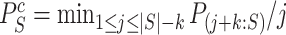 and
and  is defined as in (4). Now the calculation of the adjusted
  -value is completely analogous to the calculation of adjusted
  -values for individual features in Hommel’s procedure as given in [48]. The adjusted
  -values for
  is therefore given by
 |
(5) |
where  and
and  .
.
Simulation experiment set-up
We designed a small simulation experiment to evaluate the power of the unified approach. Our aim is not to show that the new method is more powerful than existing self-contained or competitive methods. If fact, we expect many such methods to be more powerful because they do not offer the same flexibility that our approach offers. Our aim is merely to show that the proposed method has comparable power to commonly used approaches. Therefore, we did not conduct an exhaustive simulation with many competing approaches, but compared only with the most popular and basic method, which is the Fisher’s exact test. Among enrichment methods, Fisher’s exact test is most comparable with ARI because the two methods have the same definition of enrichment: an increased proportion of active features. There are many simulations comparing Fisher’s exact test to competing methods, which can be used for cross-comparisons [49,50].
The simulation set-up is as follows: we defined 24500 features based on ENSEMBL identifiers. The GO database was used to make 12252 feature sets. For each simulation, a small (50), moderate (100) or large (200) pathway was selected randomly as the active pathway. The proportion of active features in the active pathway and in the background varied between 0.1, 0.3, 0.5 and 0, 0.05, 0.1, respectively. These proportions were held fixed, but the precise active genes were randomly selected. We generated  -scores for each feature independently. For the non-active features, these were standard normally distributed. For active features,
  -scores were assumed to follow a normal distribution with mean
  2, 3, 4 or 5, and unit variance. From the
  -scores, we calculated the corresponding one-sided
  -values. Varying all 5 parameters over the values mentioned led to 108 scenarios in total. For each scenario, the adjusted
  -value of the truly active set was calculated for our novel competitive test and for Fisher’s test. In the latter case, we corrected for multiple testing of 12252 GO terms using 2 approaches. FDR was controlled using BH method, and FWER was controlled using Hommel’s method. Power was defined as the proportion of adjusted
  -values
  for our assumed truly active set in 1000 repetitions. Results of the simulation are presented in Figure 3 and Supplementary Figures 3 and 4. R source code that was used for simulations is also provided in the supplementary data.
Figure 3.

Simulation results. Power to detect a moderate-sized pathway (100 features) truly active feature set is compared for the three approaches. In general, power of Fisher’s exact test with FDR and FWER corrections is the same, so the corresponding line appears as a single dot-dashed line. When there are no active features in the background, the three methods have very similar power. As the difference between set and background TDP decreases, ARI gains power compared to Fisher’s exact test.
Implementation
The following data analysis pipeline based on SEA approach, includes simple steps, but provides powerful error control and flexibility. All the mentioned calculations can be done through the rSEA R package that has the ARI algorithms.
The required input is simply the features with their feature-wise  -values. For any collection of feature sets of choice, the researcher obtains the estimate and confidence bound for the proportion of active features, as well as the adjusted
  -values for any value of
  , two default options are zero and estimated overall TDP value.
Figure 1 portrays the pipeline graphically. As emphasized in the figure, users may iterate the procedure as many times as they like, reconsidering the choice of database as well as the value of  . All reported results have guaranteed FWER control regardless of the number of hypotheses or the number of iterations.
Figure 1.

Suggested pipeline for testing feature sets in genomics. Solid lines are mandatory, e.g. confidence bounds are always used to test the unified null hypothesis. Dashed lines can be repeated as needed, e.g. defining  based on a different threshold values
  is allowed. Dotted lines are optional, e.g. set
  may be selected based on biological knowledge, data set, both or neither.
Results
DMD study
The data from a mouse model for Duchenne muscular dystrophy (DMD) have been used to illustrate the application of our method in the context of an RNA-seq experiment. For a more detailed description of the data set and analysis steps, refer to supplementary data. Count data were pre-processed and analyzed conventionally. Feature-wise  -values were computed based on a linear model for 13985 features. The estimated proportion of overall active features in the data set was 0.235. An enrichment analysis was performed based on SEA and simultaneous 0.05-level confidence bounds were built for the
  possible sets. Using these confidence bounds, we tested the unified null,
  , for two thresholds,
  and
and  , and 13278 feature-sets
  . By setting the threshold to zero,
  tests the self-contained null hypothesis. Setting 0.235, it will resemble the competitive null hypothesis. Feature sets were defined based on the mice pathways from GO (11881 sets), Reactome (1188 sets) and WikiPathways (209 sets) databases.
A proper enrichment method should not depend on the size of the pathway. We checked this property by plotting the adj. -values from SEA with
  against pathway sizes for all pathways from the three databases. As illustrated in Figure 2, the
  -values are not associated with the pathway size.
Figure 2.

The log  -values obtained from testing the unified null hypothesis,
  , are plotted against the size of pathway S. There is no clear relationship between the two variables.
Figure 1 shows significantly enriched (competitive adj.  -value
 ) pathways from WikiPathways based on SEA. The SEA chart provides detailed information regarding the path size, proportion of active genes and the test results. For instance, oxidative damage includes 41 genes. In this data, 37 (
 ) of these genes are studied. The estimated lower bound for the proportion of active genes is 0.27. So, there are at least 10 (=
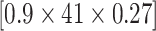 ) differentially expressed genes in this pathway. The unified null hypothesis
  oxidative damage
 is rejected with an adjusted
  -value of 0.038. This was expected as the lower bound and the point estimate (0.351) is greater than the threshold. Actually, as all pathways in this table are significantly enriched, all the estimated values of TDP bounds are greater than the threshold. On the other hand, according to the adjusted
  -value for the self-contained test (
 ), all these pathways include at least one active gene. This statement is true for 169 sets (out of 209 sets) from WikiPathways, making it hard to specify outcome-related pathways. Similar tables for Reactome and GO databases are provided in supplementary data (Supplementary Tables 1 and 2).
Table 1.
SEA chart for enriched sets from WikiPathways database
| Pathway name | Size | Coverage | TDP bound | TDP estimate | Self-contained adj.  -value -value |
Competitive adj.  -value -value |
|---|---|---|---|---|---|---|
| Irinotecan pathway | 10 | 0.40 | 0.500 | 0.500 |

|

|
| Microglia pathogen phagocytosis pathway | 41 | 0.95 | 0.487 | 0.539 |

|

|
| Macrophage markers | 10 | 1 | 0.600 | 0.800 |

|

|
| TYROBP causal network | 58 | 0.97 | 0.571 | 0.607 |

|
0.001 |
| Statin pathway | 19 | 0.63 | 0.333 | 0.333 |

|
0.002 |
| Fatty acid beta oxidation (streamlined) | 32 | 0.81 | 0.423 | 0.577 |

|
0.007 |
| Matrix metalloproteinases | 29 | 0.69 | 0.350 | 0.350 |

|
0.007 |
| Fatty acid beta oxidation | 34 | 0.88 | 0.400 | 0.567 |

|
0.008 |
| Nuclear receptors in lipid metabolism and toxicity | 30 | 0.60 | 0.389 | 0.389 |

|
0.009 |
| Mitochondrial LC-fatty acid beta-oxidation | 16 | 1 | 0.438 | 0.563 | 0.003 | 0.012 |
| Oxidative damage | 41 | 0.90 | 0.270 | 0.351 |

|
0.038 |
Furthermore, each gene set was divided into two portions, up-regulated and down-regulated, based on the log-fold change values. A similar pathway analysis was performed for each portion. The corresponding unified null hypotheses were tested against 0.181 and 0.216, which are the overall proportion of active up- and down-regulated features in the data, respectively. The estimated proportion of active genes for some pathways from each database, separate for up- and down-regulated genes, are presented in supplementary data (Supplementary Figures 1-3). Note that, even though these additional pathways were defined based on data, FWER is still controlled as discussed earlier.
To dive into the details of the analysis, we only considered the competitive results. Feature sets from WikiPathways mapped to inflammation, oxidative damage and fatty acid oxidation, which are known to be affected in DMD [51–55]. These pathways are highly relevant not only to explain the Duchenne pathophysiology but also to understand the treatment mechanism. DMD patients receive chronic treatment with corticosteroids, which reduces inflammation, and multiple drugs are in development to reduce the oxidative stress. Among the significantly enriched sets with only up- or down-regulated features, we found muscle contraction, focal adhesion, Akt/mTOR pathway, type II interferon signalling, oxidative stress, (lung) fibrosis, toll-like receptor signalling and FAS pathway, which are also known to be affected in DMD [52, 56–60]. The unified null hypothesis was rejected for the up-regulated portion of miRNA regulation of DNA damage pathway; at least %20 of the 45 up-regulated features in the pathway were active. Among the 137 significant sets from Reactome, there were four sets related to DNA damage, namely: G2/M DNA damage checkpoint, recognition of DNA damage by PCNA-containing replication complex, p53-dependent G1 DNA damage response and DNA damage recognition in GG-NER. A similar pattern was observed in GO database. The intrinsic apoptotic signaling pathway in response to DNA damage by p53 class mediator was found to be over-represented in the proportion of active genes. Pathways identified by WikiPathways were mirrored in Reactome including degradation of the extracellular matrix, VEGF pathway, activation of matrix metalloproteinases and pyruvate metabolism [61–64].
Further matching to the Reactome database showed interesting associations with e.g. molecules associated with elastic fibers, among which the latent TGF- binding proteins are known. Interestingly, it has been recently reported that latent TGF-
 binding protein 4 can modify the course of the diseases in dystrophic mice and patients [65,
66].
binding protein 4 can modify the course of the diseases in dystrophic mice and patients [65,
66].
Reactome mapping highlighted how DCC signalling is affected in mdx mice. Members of this pathway such as neogenin have been shown to promote muscle fiber formation in vitro [67], which can be connected to the capacity of muscle to regenerate and form new muscle fibers. The DCC pathway is involved in axon attraction. Other pathways providing evidence of axon growth were found to be significant in the Reactome database such as L1 signal transduction, which can act via NF- B signalling [68]. Another significant association with the Reactome database showed involvement of the unfolded protein response with pathways such as calnexin/calreticulin cycle. This observation is in line with a recent paper showing how the unfolded protein response is specifically affected in mdx mice [69]. Interestingly, five significant pathways from Reactome involved Runx2 and Runx3, which have not been linked to Duchenne in literature. Studies are required to unravel the potential link between these proteins and the pathophysiology of DMD. The 56 enriched GO terms were mostly referring to inflammation, immune reaction, myogenesis and energy production supporting the findings from WikiPathway and Reactome. Detailed GO pathways clarified that cytokines and T cells are mainly at the core in the inflammatory process as shown in the literature [70].
Power comparison
We performed a simulation experiment as described in Simulation Experiment Set-up to compare power properties of SEA with Fisher’s exact test. Despite the flexibility of SEA, we found it to have acceptable power over the whole range of simulation scenarios. We present the results for a moderate (100 features) feature set in Figure 3. Small (50 features) and large (200 features) feature sets follow a similar pattern, and the corresponding graphs can be found in the supplementary data (Supplementary Figures 4 and 5).
First, we note that FDR (BH) or FWER control (Bonferroni) hardly matters for the Fisher’s exact test approach. This was expected since only one highly enriched set was assumed. All three approaches successfully control the type I error rate at 0.05 under the null hypothesis, as shown in the bottom left panel. This is natural as all simulation scenarios use independent  -values, so both methods are valid. As expected, power for both Fisher’s exact test and for ARI increases as the effect-size
  per feature increases and as the difference between set TDP and background TDP increases. In case of no active features in the background, the methods have remarkably similar power. Differences in power occur when there is signal in the background. Fisher’s exact test has great difficulty detecting small differences between set and background TDP: even when all active features are detected as active the Fisher exact
  -value is not always small enough to survive the multiple testing correction. On the other hand, Fisher’s exact test starts to gain over ARI if this difference in signal between feature set and background becomes large. For larger or smaller feature sets (results shown in the supplemental information), we can say that power for both methods is lower for small feature sets than for large ones. ARI loses less power over Fisher’s exact test if the feature set gets smaller but conversely gains less if the feature set gets larger.
To properly interpret the results of the simulation, we should emphasize that the methods are not really comparable because the way they handle multiple testing is so different. On the one hand, 12252 feature sets is a large number, leading to a heavy multiple testing burden for Fisher’s exact test. In some applications, the number of tests may be smaller, leading to more power for Fisher’s exact test. In this sense, the simulation can be seen as unfavorable to Fisher’s exact test. On the other hand, ARI actually corrects for multiple testing for 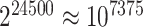 feature sets, while Fisher’s exact test is only required to correct for 12252. In this sense, the simulation experiment is unfavorable to ARI.
Discussion
We have introduced a novel paradigm for enrichment analysis of feature sets. It combines the pre-existing self-contained and competitive approaches by defining a unified null hypothesis that includes the null hypotheses of both approaches as special cases. This null hypothesis is tested with ARI, an approach to multiple testing that controls FWER based on closed testing and Simes tests.
The new approach is extremely flexible. Not only does it allow both self-contained and competitive testing but also it allows the user to choose the type of test after seeing the data, namely competitive or self-contained. Moreover, the choice of feature-set database(s) may also be postponed until after seeing the data. The data may even be used for the definition of feature sets, e.g. by taking subsets of feature sets with a certain sign or magnitude of estimated effect. Users may even iterate and revise the choice of type of test and the definition of feature sets of interest on the basis of ARI’s results. Still, family-wise error is controlled for all final results. Family-wise error is even controlled for future looks, i.e. new feature sets that could be of interest at some later stage. The method controls for all feature sets of all sizes, including singleton sets, so that it avoids inflated error rates caused by separately testing feature sets and single features.
Notably, post hoc choice of the test value  adds even more flexibility for different study goals. Larger
  values will result in a smaller list of highly enriched feature sets, appropriate for data with many active features. In contrast, smaller
  will result in a longer list of potentially relevant feature sets, a desired property for exploratory studies. The estimated value of
  is a good starting value, but we emphasize that
  may be freely tuned after seeing the data.
Allowing post hoc tuning of  circumvents a fundamental problem of competitive testing as it is classically defined. The proportion
  of active genes in the background is very difficult to bound from below: it could be that all features in
  have a non-zero but negligible effect. In that case, we would have
  , so that the competitive null hypotheses is true, even if many more features in
  than in
  have detected signal. Rejecting the competitive null hypothesis, therefore, requires proving that
  , which in turn means proving the null hypothesis for at least some of the features in
  . In most statistical models, proving a null hypothesis is impossible without strong additional assumptions. The unified null hypothesis does not suffer from the same problem since it uses a fixed threshold
  . When rejecting the unified null hypothesis at the threshold
  , we should realize that we did not reject the competitive null hypothesis—which is impossible—but we simply proved that the percentage of activation is at least
  . Proving this is as close as we can get to true competitive testing.
The new method uses only feature-wise  -values as input, so that it can be used with any omics platform, experimental design or model. ARI combines
  -values using the Simes test. The only assumption needed is therefore the Simes inequality, which allows dependence between
  -values, which is a much less restrictive assumption than the independence assumption that is invariably made by competitive methods. It is the same assumption that is needed for the validity of the procedure of BH as a method for FDR control. To the best of our knowledge, our novel approach is the only enrichment approach with proper error control in the presence of dependence between features.
Despite the flexibility and lack of independence assumptions, the new method has acceptable power compared to classical enrichment methods. Notably, the power of the method does not depend on the number of feature sets tested. As a consequence, classical methods will do better for a limited number of candidate feature sets, while ARI outperforms other methods when databases are large. In a simulation study, we found ARI to be comparable in power to a classical method for a database the size of GO. SEA is especially recommended when many feature sets are of interest or when such feature sets cannot be specified before seeing the data.
Importantly, ARI provides for each feature set not only an adjusted  -value for enrichment but also a simultaneous lower confidence bound to the actual proportion of active features. Users obtain not just the presence or absence of enrichment but also an honest assessment of the level of enrichment in each feature set.
A drawback of ARI may be that it is very strict, as it only has FWER control. For large values of  , this is not much of a drawback, as only few hypotheses will be false, so the difference between family-wise error and FDR is small. For smaller values of
  , power could be gained by switching to control of FDRs or related measures. This is left to future method development.
Application of the method is fast, and the complexity of all computations is linear or nearly linear in the number of features. An implementation of ARI is available in the rSEA package in R with some practical functions to make use of three genomics databases (GO, Reactome and WikiPathways).
Key Points
-

A unified null hypothesis states that ‘The proportion of the truly active genes in the gene set of interested is less than c.’
-

Self-contained and competitive null hypotheses are special cases of the unified null hypothesis.
-

SEA of all gene sets is possible by testing the unified null within closed testing framework.
-

Closed testing provides an FWER control over all possible gene sets. Therefore, SEA does not require a priori selection of the gene sets of the interest.
-

A main advantage of SEA over current methods is the freedom in choices of both feature set of interest and threshold c. Moreover, it is possible to revise or make new choices even after seeing the data without type I error inflation.
-

The application of SEA is not limited to gene-set analysis.
Supplementary Material
Mitra Ebrahimpoor is a PhD student at the Medical Statistics section, Department of Biomedical Data Sciences, Leiden University Medical Center. Her research focuses on statistical methods for high-dimensional data especially genomics.
Pietro Spitali is an assistant professor at the Department of Human Genetics, Leiden University Medical Center. His research focuses on the identification of biomarkers for neuromuscular disorders.
Kristina M. Hettne is a digital scholarship librarian at Center for Digital Scholarship, Leiden University Library.
Roula Tsonaka is an assistant professor at the Medical Statistics section, Department of Biomedical Data Sciences, Leiden University Medical Center. Her research focuses on statistical methods for longitudinal omics data.
Jelle J. Goeman is a professor at the Medical Statistics section, Department of Biomedical Data Sciences, Leiden University Medical Center. His research focuses on methods for large multiple hypothesis testing problems with applications in gene expression and neuroscience.
Funding
Netherlands Organization for Scientific Research VIDI (639.072.412); European Community’s Seventh Framework Programme (FP7-Health) (305121 to P.S.); Integrated European Project on Omics Research of Rare Neuromuscular and Neurodegenerative Diseases (NEUROMICS) (P.S.).
References
- 1. Subramanian A, Tamayo P, Mootha VK,. et al. Gene set enrichment analysis: a knowledge-based approach for interpreting genome-wide expression profiles. Proc Natl Acad Sci U S A 2005;102(43):15545–50. [DOI] [PMC free article] [PubMed] [Google Scholar]
- 2. Goeman JJ, Mansmann U. Multiple testing on the directed acyclic graph of gene ontology. Bioinformatics 2008;24(4): 537–44. [DOI] [PubMed] [Google Scholar]
- 3. Saunders G, Stevens JR, Isom SC. A shortcut for multiple testing on the directed acyclic graph of gene ontology. BMC Bioinformatics 2014;15(1):349. [DOI] [PMC free article] [PubMed] [Google Scholar]
- 4. Meijer RJ, Goeman JJ. Multiple testing of gene sets from gene ontology: possibilities and pitfalls. Brief Bioinform 2016;17(5):808–18. [DOI] [PubMed] [Google Scholar]
- 5. Gene Ontology Consortium Gene Ontology Consortium: going forward. Nucleic Acids Res 2015;43(D1):D1049–D1056. [DOI] [PMC free article] [PubMed] [Google Scholar]
- 6. Kanehisa M, Goto S. KEGG: Kyoto Encyclopedia of Genes and Genomes. Nucleic Acids Res 2000;28(1):27–30. [DOI] [PMC free article] [PubMed] [Google Scholar]
- 7. Liberzon A, Subramanian A, Pinchback R,. et al. Molecular signatures database (MSigDB) 3.0. Bioinformatics 2011;27(12):1739–40. [DOI] [PMC free article] [PubMed] [Google Scholar]
- 8. Thomas PD, Campbell MJ, Kejariwal A,. et al. PANTHER: a library of protein families and subfamilies indexed by function. Genome Res 2003;13(9):2129–41. [DOI] [PMC free article] [PubMed] [Google Scholar]
- 9. Kutmon M, Riutta A, Nunes N,. et al. WikiPathways: capturing the full diversity of pathway knowledge. Nucleic Acids Res. 2016;44(D1):D488–D494. [DOI] [PMC free article] [PubMed] [Google Scholar]
- 10. Rahmatallah Y, Emmert-Streib F, Glazko G. Comparative evaluation of gene set analysis approaches for RNA-Seq data. BMC Bioinformatics 2014;15(1):397. [DOI] [PMC free article] [PubMed] [Google Scholar]
- 11. Mooney MA, Wilmot B. Gene set analysis: a step-by-step guide. Am J Med Genet B Neuropsychiatr Genet 2015;168(7): 517–27. [DOI] [PMC free article] [PubMed] [Google Scholar]
- 12. Goeman JJ, Bühlmann P. Analyzing gene expression data in terms of gene sets: methodological issues. Bioinformatics 2007;23(8):980–7. [DOI] [PubMed] [Google Scholar]
-
13.
Fisher RA.
On the interpretation of
 2 from contingency tables, and the calculation of P. J R Stat Soc 1922;85(1):87. [Google Scholar]
 - 14. Efron B, Tibshirani R. On testing the significance of sets of genes. Ann Appl Stat 2007;1(1):107–129. [Google Scholar]
- 15. Barry WT, Nobel AB, Wright FA. Significance analysis of functional categories in gene expression studies: a structured permutation approach. Bioinformatics 2005;21(9):1943–1949. [DOI] [PubMed] [Google Scholar]
- 16. Goeman JJ, Van de Geer SA, De Kort F, Van Houwelingen HC. A global test for groups of genes: testing association with a clinical outcome. Bioinformatics 2004;20(1):93–9. [DOI] [PubMed] [Google Scholar]
- 17. Hummel M, Meister R, Mansmann U. GlobalANCOVA: exploration and assessment of gene group effects. Bioinformatics 2008;24(1):78–85. [DOI] [PubMed] [Google Scholar]
- 18. Pedroso I, Lourdusamy A, Rietschel M,. et al. Common genetic variants and gene-expression changes associated with bipolar disorder are over-represented in brain signaling pathway genes. Biol. Psychiatry 2012;72(4):311–317. [DOI] [PubMed] [Google Scholar]
- 19. Michael CW, Lin X. Prior biological knowledge-based approaches for the analysis of genome-wide expression profiles using gene sets and pathways. Stat Methods Med Res 2009;18(6):577–93. [DOI] [PMC free article] [PubMed] [Google Scholar]
- 20. de Leeuw CA, Neale BM, Heskes T, Posthuma D. The statistical properties of gene-set analysis. Nat Rev Genet 2016;17(6):353–64. [DOI] [PubMed] [Google Scholar]
- 21. Ho DWH, Ng IOL. uGPA: unified Gene Pathway Analyzer package for high-throughput genome-wide screening data provides mechanistic overview on human diseases. Clin Chim Acta 2015;441:105–8. [DOI] [PubMed] [Google Scholar]
- 22. Wu D, Smyth GK. Camera: a competitive gene set test accounting for inter-gene correlation. Nucleic Acids Res 2012, 40(17):e133. [DOI] [PMC free article] [PubMed] [Google Scholar]
- 23. Newton MA, Wang Z. Multiset statistics for gene set analysis. Annu Rev Stat Appl 2015;2(1):95–111. [DOI] [PMC free article] [PubMed] [Google Scholar]
- 24. Maciejewski H. Gene set analysis methods: statistical models and methodological differences. Brief Bioinform 2014;15(4):504–18. [DOI] [PMC free article] [PubMed] [Google Scholar]
- 25. Debrabant B. The null hypothesis of GSEA, and a novel statistical model for competitive gene set analysis. Bioinformatics 2017;33(9):1271–7. [DOI] [PubMed] [Google Scholar]
- 26. Benjamini Y, Heller R. Screening for partial conjunction hypotheses. Biometrics 2008;64(4):1215–22. [DOI] [PubMed] [Google Scholar]
- 27. Goeman JJ, Solari A. Multiple testing for exploratory research. Stat Sci 2011;26(4):584–97. [Google Scholar]
- 28. Goeman J, Meijer R, Krebs T,. et al. Simultaneous control of all false discovery proportions in large-scale multiple hypothesis testing. 2016. arXiv:1611.06739v2.
- 29. Marcus R, Eric P, Gabriel KR. On closed testing procedures with special reference to ordered analysis of variance. Biometrika 1976;63(3):655–60. [Google Scholar]
- 30. Simes RJ. An improved Bonferroni procedure for multiple tests of significance. Biometrika 1986;73(3):751–4. [Google Scholar]
- 31. Rosenblatt JD, Finos L, Weeda WD,. et al. All-Resolutions Inference for brain imaging. Neuroimage 2018;181:786–796. [DOI] [PubMed] [Google Scholar]
- 32. Benjamini Y, Hochberg Y. Controlling the false discovery rate: a practical and powerful approach to multiple testing. J R Stat Soc Series B Stat Methodol 1995;57:289–300. [Google Scholar]
- 33. Rahmatallah Y, Emmert-Streib F, Glazko G. Gene set analysis approaches for RNA-seq data: performance evaluation and application guideline. Brief Bioinform 2016;17(3): 393–407. [DOI] [PMC free article] [PubMed] [Google Scholar]
- 34. Nam D, Kim SY. Gene-set approach for expression pattern analysis. Brief Bioinform 2008;9(3):189–97. [DOI] [PubMed] [Google Scholar]
- 35. Tripathi S, Glazko GV, Emmert-Streib F. Ensuring the statistical soundness of competitive gene set approaches: gene filtering and genome-scale coverage are essential. Nucleic Acids Res 2013;41(7):e82. [DOI] [PMC free article] [PubMed] [Google Scholar]
- 36. Boca SM, Bravo HC, Caffo B,. et al. A decision-theory approach to interpretable set analysis for high-dimensional data. Biometrics 2013;69(3):614–23. [DOI] [PMC free article] [PubMed] [Google Scholar]
- 37. Breitling R, Amtmann A, Herzyk P. Iterative Group Analysis (iGA): a simple tool to enhance sensitivity and facilitate interpretation of microarray experiments. BMC Bioinformatics 2004;5(1):34. [DOI] [PMC free article] [PubMed] [Google Scholar]
- 38. Väremo L, Nielsen J, Nookaew I. Enriching the gene set analysis of genome-wide data by incorporating directionality of gene expression and combining statistical hypotheses and methods. Nucleic Acids Res 2013;41(8):4378–91. [DOI] [PMC free article] [PubMed] [Google Scholar]
- 39. Gatti DM, Barry WT, Nobel AB,. et al. Heading down the wrong pathway: on the influence of correlation within gene sets. BMC Genomics 2010;11(1):574. [DOI] [PMC free article] [PubMed] [Google Scholar]
- 40. Wang L, Jia P, Wolfinger RD,. et al. Gene set analysis of genome-wide association studies: methodological issues and perspectives. Genomics 2011;98(1):1–8. [DOI] [PMC free article] [PubMed] [Google Scholar]
- 41. Tarca AL, Bhatti G, Romero R,. et al. A comparison of gene set analysis methods in terms of sensitivity, prioritization and specificity. Plos One 2013;8(11): e79217. [DOI] [PMC free article] [PubMed] [Google Scholar]
- 42. Sarkar SK. On the Simes inequality and its generalization. Beyond Parametrics in Interdisciplinary Research: Festschrift in Honor of Professor Pranab K. Sen. Beachwood, Ohio, USA: Institute of Mathematical Statistics, 2008,231–42. [Google Scholar]
- 43. Sabatti C, Service S, Freimer N. False discovery rate in linkage and association genome screens for complex disorders. Genetics 2003;164(2):829–33. [DOI] [PMC free article] [PubMed] [Google Scholar]
- 44. Benjamini Y, Yekutieli D. The control of the false discovery rate in multiple testing under dependency. Ann Statist 2001;29:1165–88. [Google Scholar]
- 45. Rodland EA. Simes’ procedure is ”valid on average”. Biometrika 2006;93(3):742–6. [Google Scholar]
- 46. Finner H, Roters M, Strassburger K. On the Simes test under dependence. Statist Papers 2017;58(3):775–89. [Google Scholar]
- 47. Su WJ. The FDR-linking theorem. 2018. arXiv:1812.08965.
- 48. Meijer RJ, Krebs TJP, Goeman JJ. Hommel’s procedure in linear time. Biom J 2019;61(1):73–82. [DOI] [PubMed] [Google Scholar]
- 49. Tryputsen V, Cabrera J, De Bondt A, Amaratunga D. Using Fisher’s method to identify enriched gene sets. Stat Biopharm Res 2014;6(2):154–162. [Google Scholar]
- 50. Glass K, Girvan M. Annotation enrichment analysis: an alternative method for evaluating the functional properties of gene sets. Sci Rep 2015;4(1):4191. [DOI] [PMC free article] [PubMed] [Google Scholar]
- 51. Lin CH, Hudson AJ, Strickland KP. Fatty acid oxidation by skeletal muscle mithochondria in duchenne dystrophy. Life Sciences 1972;11(7):355–62. [DOI] [PubMed] [Google Scholar]
- 52. Murphy ME, Kehrer JP. Oxidative stress and muscular dystrophy. Chem Biol Interact 1989;69(2–3):101–73. [DOI] [PubMed] [Google Scholar]
- 53. Nakagawa T, Takeuchi A, Kakiuchi R,. et al. A prostaglandin D2 metabolite is elevated in the urine of Duchenne muscular dystrophy patients and increases further from 8 years old. Clin Chim Acta 2013;423:10–14. [DOI] [PubMed] [Google Scholar]
- 54. del Rocío Cruz-Guzmán O, Rodríguez-Cruz M, Escobar Cedillo RE. Systemic inflammation in Duchenne muscular dystrophy: association with muscle function and nutritional status. Biomed Res Int 2015;2015:1–7. [DOI] [PMC free article] [PubMed]
- 55. Vianello S, Pantic B, Fusto A,. et al. SPP1 genotype and glucocorticoid treatment modify osteopontin expression in Duchenne muscular dystrophy cells. Hum Mol Genet 2017;26(17):3342–3351. [DOI] [PubMed] [Google Scholar]
-
56.
Villalta SA, Deng B, Rinaldi C,.
et al.
IFN-
 promotes muscle damage in the mdx mouse model of Duchenne muscular dystrophy by suppressing M2 macrophage activation and inhibiting muscle cell proliferation. J Immunol 2011;187(10):5419–28. [DOI] [PMC free article] [PubMed] [Google Scholar]
 - 57. de Morrée A, Hensbergen PJ, Herman HHBM, van Haagen BM,. et al. Proteomic analysis of the Ddysferlin protein complex unveils its importance for sarcolemmal maintenance and integrity. PLoS One 2010;5(11): e13854. [DOI] [PMC free article] [PubMed] [Google Scholar]
- 58. Mojumdar K, Giordano C, Lemaire C,. et al. Divergent impact of Toll-like receptor 2 deficiency on repair mechanisms in healthy muscle versus Duchenne muscular dystrophy. J Pathol 2016;239(1):10–22. [DOI] [PubMed] [Google Scholar]
-
59.
Taniguti APT, Pertille A, Matsumura C,.
et al.
Prevention of muscle fibrosis and myonecrosis in mdx mice by suramin, a TGF-
 1 blocker. Muscle Nerve 2011;43(1):82–87. [DOI] [PubMed] [Google Scholar]
 - 60. Spitali P, Grumati P, Hiller M,. et al. Autophagy is impaired in the tibialis anterior of dystrophin null mice. PLoS Curr 2013;5 10.1371/currents.md.e1226cefa851a2f079bbc406c0a21e80 [DOI] [PMC free article] [PubMed] [Google Scholar]
- 61. Hindi SM, Shin J, Ogura Y,. et al. Matrix metalloproteinase-9 inhibition improves proliferation and engraftment of myogenic cells in dystrophic muscle of mdx mice. PLoS One 2013;8(8): e72121. [DOI] [PMC free article] [PubMed] [Google Scholar]
- 62. Dahiya S, Bhatnagar S, Hindi SM,. et al. Elevated levels of active matrix metalloproteinase-9 cause hypertrophy in skeletal muscle of normal and dystrophin-deficient mdx mice. Hum Mol Genet 2011;20(22):4345–4359. [DOI] [PMC free article] [PubMed] [Google Scholar]
- 63. Lourbakos A, Yau N, de Bruijn P,. et al. Evaluation of serum MMP-9 as predictive biomarker for antisense therapy in Duchenne. Sci Rep 2017;7(1):17888. [DOI] [PMC free article] [PubMed] [Google Scholar]
- 64. Pant M, Sopariwala DH, Bal NC,. et al. Metabolic dysfunction and altered mitochondrial dynamics in the utrophin-dystrophin deficient mouse model of Duchenne muscular dystrophy. PLoS One 2015;10(4): e0123875. [DOI] [PMC free article] [PubMed] [Google Scholar]
- 65. Flanigan KM, Ceco E, Lamar KM,. et al. LTBP4 genotype predicts age of ambulatory loss in Duchenne muscular dystrophy. Ann Neurol 2013;73(4):481–8. [DOI] [PMC free article] [PubMed] [Google Scholar]
- 66. Van Den Bergen JC, Hiller M, Bohringer S,. et al. Validation of genetic modifiers for Duchenne muscular dystrophy: a multicentre study assessing SPP1 and LTBP4 variants. J Neurol Neurosurg Psychiatry 2015;86(10):1060–5. [DOI] [PMC free article] [PubMed] [Google Scholar]
- 67. Kang JS, Yi MJ, Zhang W,. et al. Netrins and neogenin promote myotube formation. J Cell Biol 2004;167(3):493–504. [DOI] [PMC free article] [PubMed] [Google Scholar]
-
68.
Kiefel H, Pfeifer M, Bondong S,.
et al.
Linking L1CAM-mediated signaling to NF-
 B activation. Trends Mol Med 2011;17(4):178–187. [DOI] [PubMed] [Google Scholar]
 - 69. Hulmi JJ, Hentilä J, DeRuisseau KC,,. et al. Effects of muscular dystrophy, exercise and blocking activin receptor IIB ligands on the unfolded protein response and oxidative stress. Free Radic Biol Med 2016;99:308–22. [DOI] [PubMed] [Google Scholar]
- 70. Villalta SA, Rosenberg AS, Bluestone JA. The immune system in Duchenne muscular dystrophy: friend or foe. Rare Dis 2015;3(1): e1010966. [DOI] [PMC free article] [PubMed] [Google Scholar]
Associated Data
This section collects any data citations, data availability statements, or supplementary materials included in this article.