Single-Cell Classification Using Mass Spectrometry Through Interpretable Machine Learning

Abstract

The brain consists of organized ensembles of cells that exhibit distinct morphologies, cellular connectivity and dynamic biochemistries that control the executive functions of an organism. However, the relationships between chemical heterogeneity, cell function, and phenotype are not always understood. Recent advancements in matrix-assisted laser desorption/ionization mass spectrometry have enabled the high-throughput, multiplexed chemical analysis of single cells, capable of resolving hundreds of molecules in each mass spectrum. We developed a machine learning workflow to classify single cells according to their mass spectra based on cell groups of interest (GOI), e.g., neurons vs. astrocytes. Three datasets from various cell groups were acquired on three different mass spectrometer platforms representing thousands of individual cell spectra were collected and used to validate the single cell classification workflow. The trained models achieved >80% classification accuracy and were subjected to the recently developed instance-based model interpretation framework, SHAP (SHapley Additive exPlanations), which locally assigns feature importance for each single-cell spectrum. SHAP values were used for both local and global interpretations of our datasets, preserving the chemical heterogeneity uncovered by the single-cell analysis while offering the ability to perform supervised analysis. The top contributing mass features to each of the GOI were ranked and selected using mean absolute SHAP values, highlighting the values that are specific to the defined GOI. Our approach provides insight into discriminating the chemical profiles of the single cells through interpretable machine learning, facilitating downstream analysis and validation.

Graphical Abstract

INTRODUCTION

Single-cell chemical analysis enables the identification of unique cellular markers based on known phenotypes and physiological states, and provides the opportunity to search for rare biological events that contribute to cellular abnormalities. Single-cell RNA sequencing (scRNA-seq) has been the method of choice to study cellular heterogeneity and its impact on the structural organization and function of complex multicellular structures, such as the nervous system. Lipids are a structurally diverse and important class of molecules in the brain, comprising 50–60% of its dry weight, and disruption to lipid homeostasis can lead to progressive degeneration of neurons^1,2 In addition, small metabolites such as neurotransmitters are crucial to neurological function.³ The molecular mechanisms governing the transcriptional control of lipids and detailed information on brain metabolomics are not well understood. Therefore approaches that provide direct information on the chemical contents of cells are important.^4–7 Recent advancements in matrix-assisted laser desorption/ionization (MALDI) mass spectrometry (MS) have enabled the high-throughput analysis of single cells and the detection.^8–13 MALDI MS can be coupled to other techniques, such as immunocytochemistry (ICC),¹⁴ to screen thousands of cells labeled by their canonical cell types, producing information-rich ‘omics’ data on the peptidome, lipidome and metabolome. Although not yet commonly employed, many exploratory computational tools that are available for scRNA-seq,¹⁵ such as unsupervised analysis for exploratory data analysis,¹⁶ can be adapted to MALDI MS measurements for determination of the chemical differences between single cells and cell types.

The processed single-cell mass spectra can be treated as a multi-dimensional dataset, allowing the application of multivariate data analysis methods, such as principal component analysis (PCA), to enable the analysis and visualization of high-dimensional datasets of related cell populations based on their discriminating mass spectral features. Additionally, distinct algorithms have been applied to single-cell MS datasets, including t-SNE, for visualizing high-dimensional data through nonlinear dimension reduction.^9,12,14,17 The application of such algorithms for single-cell MS data analysis has become integral to research pipelines.¹⁸ However, MALDI MS can be sensitive to non-biological variations, such as shot-to-shot and spot-to-spot variability, as well as “batch effects” experienced between biological replicates.¹⁹ These experimental variations influence the output of unsupervised algorithms, which can lead to spurious clustering based on changes in experimental conditions rather than intrinsic biological differences. When mass spectra are acquired from similar samples, unwanted variations in total ion count and instrumental noise typically dominate the output of unsupervised algorithms, which we demonstrated on single-cell MALDI MS datasets. MALDI MS analyses of cerebellar neurons and astrocytes were followed by ICC cell typing and comparison of known phenotypes to single-cell mass spectral profiles.¹⁴ The first two principal components (PCs) showed that cells clustered in batches (on different days of MS analysis) instead of by cell phenotype. Unwanted variations and batch effects were still prominently featured in the PCA output of different brain regions (the hippocampus and cerebellum), which are expected to have more distinct mass spectral features.

Recent progress in machine learning has facilitated pattern recognition, classification and regression analyses that are useful for complex and noisy high-dimensional datasets.^20–23 Support vector machine (SVM), random forest (RF), and deep neural networks (DNNs) were utilized for data mining and knowledge discovery for various MALDI MS datasets,^24–29 introducing ways to overcome experimental variations to reveal the biological variability within the datasets. Interpretation of machine learning model output is important when gathering biologically relevant data. However, modern machine learning systems are often treated as “black boxes”, preventing the user from understanding how the machine learning algorithm is producing its model output, thus hindering the interpretability of the model.³⁰ Here we present a novel method to train and interpret the output of supervised classification models for single-cell MALDI MS data analysis that allows cell classification in defined GOI based on their contributing mass spectral features. In particular, ensemble tree models (Gradient Boosting Trees and random forest) were trained and the model outputs explained by SHapley Additive exPlanation (SHAP) values based on game theory to get consistent feature attributions for each individual data point (the single-cell spectra).³¹ This approach leverages cell-to-cell heterogeneity revealed by the single-cell MS analysis to provide local interpretations while following general supervised classification of GOI for global interpretations. Also, PCA was performed on feature attribution values to visualize the low-dimensional structures involved in decision making by the model for each cell, compared with the structure of the biological GOI.

We applied this method on three single-cell datasets: (1) a new dataset, consisting of 1201 single cells from different rat brain regions, hippocampus or cerebellum, at a mass range from m/z 50 to 500 acquired on a 7T Fourier transform ion cyclotron resonance (FT-ICR) mass spectrometer (HIP_CER dataset); (2) a published dataset, consisting of 1544 rat cerebellar single cells labeled by ICC to determine which cells were neurons (NF-L positive) or astrocytes (GFAP positive) at a mass range from m/z 500 to 1000 acquired using MALDI-time-of-flight (TOF)-MS (ICC dataset);¹⁴ (3) and another published dataset, consisting of 1542 single cells from different regions, the dorsal root ganglia (DRG) or cerebellum, from m/z 500 to 850 acquired using secondary ion mass spectrometry (SIMS dataset).¹⁷

EXPERIMENTAL

The experimental details on the acquisition of the newly acquired HIP_CER dataset are provided in the Supporting Information; the data processing and machine learning details were applied to the new and two previously published datasets.

Data Processing.

The newly acquired HIP_CER dataset contains single cell dissociates from two distinct rat brain regions, 686 cells from the hippocampus and 515 cells from the cerebellum, acquired on a SolariX 7T FT-ICR mass spectrometer (Bruker Corp., Billerica, MA). The ICC dataset contains 684 astrocytes and 860 neurons from rat, analyzed by an ultrafleXtreme MALDI-TOF mass spectrometer (Bruker Corp.). The SIMS dataset contains 548 single DRG cells and 994 cerebellar neurons from rat, acquired on a laboratory-modified SIMS mass spectrometer.³² Peak-picking was performed for the HIP_CER and ICC datasets to generate sparse peak data from continuous mass spectra. Peaks with a signal to noise ratio above 5 were retained. Spectra from the SIMS dataset were uniformly binned with a bin width of 0.07 Da. Peak alignment was applied for peak-picked datasets to combine individual spectra into a multivariate matrix and overcome potential mass shifts in the same peak from different spectra. For the HIP_CER dataset, acquired by FT-ICR MS, the mass resolution changes as a function of m/z values. Thus, non-uniform bins were used to align the peaks and create matrices with rows as individual cells and columns as m/z features. For example, the bin width was set as 0.001 at m/z 50 and 0.005 at m/z 500. These matrices (.mat) were imported into Python 3.7 where single-cell spectra were individually normalized by root mean square (RMS) of m/z features for the peak-picked datasets. The binned spectra from the SIMS dataset were normalized by L1 norm (sum of a vector). For both methods where x⁽ⁱ⁾={x⁽ⁱ⁾₁,x⁽ⁱ⁾_2,…_X⁽ⁱ⁾_m} with x⁽ⁱ⁾_j as the j-th m/z feature of spectrum i, the normalized spectrum x′⁽ⁱ⁾ is:

$$\text{RMS}:{\text{x}}^{\text{'(i) }}=\frac{{\text{x}}^{(\text{i})}}{\sqrt{\frac{{({\text{x}}^{(\text{i})}{}_1)}^2+{({\text{x}}^{(\text{i})}{}_2)}^2\dots +{({\text{x}}^{(\text{i})}{}_{\text{m}})}^2}{\text{m}}}}\text{L}1:{\text{x}}^{\text{'}(\text{i})}=\frac{{\text{x}}^{(\text{i})}}{{\sum }_{\text{j}=1}^{\text{m}}{\text{x}}^{\left(\text{i}\right)}{}_{\text{j}}}$$ (Eq. 1)

Mass features were selected from m/z 50 to 500, m/z 500 to 1000, and m/z 500 to 850 for the HIP_CER, ICC, and SIMS datasets, respectively, for machine learning classification. Mass features present in less than 3% of the total number of single cells were discarded. The average and subtracted spectra for the newly acquired HIP_CER dataset are provided in Figure S1.

Single-Cell Classification Through Machine Learning.

Single-cell classification is a supervised machine learning task that learns a function and maps the input data X (single-cell spectra) to the categorical output variable Y (cell GOI). The normalized intensity matrices of single-cell mass spectra were used to train classifiers to predict cell GOI using the ensemble tree models (see Supporting Information). The same procedure was applied to the three datasets individually, unless otherwise stated. The sample spectra were split into a training set and a test set with a ratio of 4:1. The relative feature importance scores were obtained through information gain (Gini importance) and plotted against m/z values (Supporting Information). The classification pipeline was implemented in Python 3.7 and the software packages, including xgboost³³ and scikit-learn,³⁴ were used for machine learning implementations. Specific hyperparameter choices are provided in the Supporting Information. Notebooks are available online for readers to reproduce the data analysis and figures in the paper (https://github.com/richardxie1119/SCCML).

Interpretable Machine Learning via SHAP Values.

Although the relative importance scores computed by Gini importance grants certain interpretability due to the hierarchical ranking of the entire feature set, Gini importance may provide inconsistent and biased feature importance measures,^31,35 which are also only available at the global scale. We thus applied a recently developed framework of SHAP³⁶ based on the additive feature attribution methods, which locally assigns consistent feature importance for each individual prediction of a single cell (see Supporting Information). SHAP values for the gradient boosting trees were computed using the Python software Tree SHAP,³¹ which implements a fast exact algorithm to compute SHAP values for tree ensemble models.

The resulting SHAP values were then subjected to interpretation. Since the SHAP values had the same dimensions as the original datasets, PCA was applied on the SHAP matrices from the three datasets to reveal the model decisions in low-dimensional space by grouping samples with similar feature contributions. SHAP values of a single cell allow local interpretations of how features contribute to a single instance model prediction, whereas the mean absolute SHAP values of features indicate their global impact toward model predictions (SHAP values can be positive or negative depending on which GOI a feature contributes to). The mean absolute SHAP values for each complete dataset were used to rank features. To select the features most important for classifying GOI and test their robustness, models were retrained using an incrementally increasing number of top-ranked features to determine model performance from the area under the curve (AUC) of the receiver operating characteristic. From this analysis, the Elbow method was used to heuristically choose the optimal number of top-ranked features. Models were then trained on the same number of features randomly sampled from the datasets (with replacement) 300 times to test how strong the selected features were as model predictors.

RESULTS AND DISCUSSION

Three datasets were used to demonstrate our method, one newly acquired (the HIP_CER dataset) and two previously published (the ICC dataset¹⁴ and the SIMS dataset¹⁷). In all cases, the ground truth condition was obtained based on spatial location of the cell dissociates for the HIP_CER (hippocampus/cerebellum cells) dataset and SIMS (DRG/cerebellum cells) dataset, or based on canonical cell types obtained from immunocytochemistry for the ICC (neurons/astrocytes) dataset.

Results from Traditional Statistical Models are Prone to Experimental Variation.

One of the most straightforward supervised analysis methods is the Wilcoxon rank-sum test (or Mann Whitney U-test), which is nonparametric and performed on the ranks of all the observations.³⁷ This test may be used to determine if the distributions of mass features were significant between single-cell GOI. Thus, a p-value was calculated for each individual peak-picked mass feature from the three datasets. In fact, most features showed low p-values, indicating distinct distributions between groups for all three datasets (Figure S2), which may also result from sensitivity of the rank-sum test to noise and unwanted variations inherent to the datasets. Overall, our interpretations of the datasets were restricted by the uninformative results provided by the rank-sum test, especially during an exploratory study in which prior knowledge was limited. Mass-match of compounds of interest is one way to narrow the range of features for the downstream analysis; however, this limits analysis to mass features that have previously been documented in available metabolite databases. As a result, important mass features without a matching mass value can easily be omitted, potentially creating a loss of information. As discussed above, performing PCA on high-dimensional, sparse datasets is not ideal as differences in instrument noise can account for the largest variance and consequently will be transformed into the principal components. Principal components based on instrumental variation can create clustering by the day of analysis (Figure 1A, B) while ignoring the actual biological variation. Other statistical methods include clustering techniques, such as K-means and Hierarchical Clustering, but may have similar limitations, with the recovered clusters representing different batches or analysis days. In response to these limitations, a dedicated field in single-cell RNA sequencing is working to eliminate unwanted variations by quantitatively and systematically evaluating the performance of different normalization procedures.³⁸ In the field of single-cell MS, efforts to create robust and informative multivariate analysis techniques are still needed.

Figure 1.

PCA on the preprocessed intensity matrices showed significant clustering of samples based on batches for both the (A) ICC dataset and the (B) HIP_CER dataset; batches with cell populations were obtained from 3 animals. The workflow of single-cell classification using high-throughput MS involves (C, top box) single population collection after enzymatic tissue dissociation, its deposition on ITO-coated glass slides, and optically guided single-cell MALDI MS data acquisition using microMS. GOI are defined either based on prior knowledge about spatial origins of the cells (e.g., cells from hippocampal or cerebellar regions) or based on ICC to identify canonical cell types (e.g., neuronal or astrocytic cells). (C, bottom box) The acquired single-cell mass spectra, after preprocessing, are then subjected to supervised machine learning to predict previously defined cell GOI. Then, the trained models are subjected to interpretation of the model output at the individual instance level (a single cell) using the recently developed SHAP framework.

Supervised Machine Learning Classifies Single-Cell GOI.

Machine learning can be applied to various tasks, including classification, in which target variables are categorical (0 and 1 for binary classification), and regression in which target variables are continuous values. Ensemble tree classifiers were trained for each dataset (Gradient Boosting Trees for the ICC and HIP_CER datasets, random forest for the SIMS dataset) based on the assumption that m/z features exist that allow the data to be classified according to the target variables (brain region or cell type). The respective datasets were split into training and testing sets for evaluation of the final model fit on the training dataset (see Experimental section). For the ICC dataset acquired using the MALDI-TOF MS instrument, the classifier was trained to differentiate between astrocytes and neurons in the rat cerebellum and achieved 0.77 accuracy on the test set. The second classifier was trained to differentiate between hippocampal and cerebellum cells using the FT-ICR MS data and was able to achieve 0.96 accuracy on the test set. Finally, for the SIMS dataset, the classifier was trained to differentiate DRG and cerebellar cells and achieved 0.99 accuracy. The overall test accuracy of the models agreed with the previous assumption that the classification models could capture the predictive m/z features for differentiating GOI.

Differences in how the single-cell data are acquired and pre-processed can influence the classification model’s output. Peaks acquired in different mass spectra that fall within a predetermined error window based on the mass error of the mass spectrometer (parts per million) are aligned and binned together. Over-binning can split a peak into multiple features, and under-binning can force multiple peaks into a single peak, ultimately influencing the number of discriminating mass features used for a classification model. The number of mass features was the greatest in the SIMS dataset (number of bins: 4688) since the spectra were resampled and uniformly binned without peak-picking. The HIP_CER dataset, which was acquired by FT-ICR MS, had the second most bin divisions and peak-picked mass features (number of features: 2464), followed by the ICC dataset acquired by MALDI-TOF MS (number of features: 512). High model performance was achieved on the HIP_CER dataset and the SIMS dataset due to the discriminative nature of cells from different anatomical regions. Relatively low performance was achieved on the ICC dataset, perhaps due to the low number of features as input for classification caused by poorer spectral quality and the heterogeneity of astrocytes and neurons. False positives caused by non-specific immunostaining can also compromise the model performance, leading to suboptimal prediction accuracy. Table 1 shows a summary of the performance scores (accuracy and AUC) of the models for three datasets.

Table 1.

Model performance scores on the test sets for three datasets.

	Accuracy	AUC
HIP_CER dataset	0.963	0.995
ICC dataset	0.774	0.833
SIMS dataset	0.995	0.996

Interpretable Machine Learning Provides Feature Attributions via SHAP Values.

For high-dimensional data, it is desirable to rank the input variables according to their relative importance to the model. Interpretations can then be made by looking at the ranked m/z features to understand which ones are relevant to the classification task. For a nonparametric statistical test, p-values obtained from the rank-sum test can be used to rank features based on how significantly different the data distributions are between groups.³⁷ In machine learning, one of the most frequently used measures for evaluating feature importance scores for ensemble tree models is the Gini feature importance, which has been applied to high-dimensional datasets such as gene expression data^39–41 and MS data^27,28 for feature selection. The Gini importance for a feature is computed by summing up its Gini impurity decrease over all trees in the forest normalized by the number of trees.⁴² The Gini importance of the three datasets was computed and visualized as stem plots, with the height representing relative feature importance (Figure S3). However, Gini importance scores are often biased in favor of variables with more possible split points.³⁵ Another feature importance measure is the permutation importance, which is the accuracy drop of the model after randomly permuting a feature in the testing set.³⁵ Both Gini importance and permutation importance measure the global impact of a feature to the model’s performance, so they do not provide information on how individual predictions are made by the model. If we are trying to understand how a prediction is made on a single-cell mass spectrum (i.e., determining the contributing features to the model prediction) by a trained ensemble tree model, the current feature importance measures may not be applicable. Recent progress in interpreting individual-instance predictions by machine learning models can be attributed to the class of additive feature attribution methods where a single-prediction output is the sum of contributions from each input feature.³⁶ One possible approach to obtain feature attributions is through computing SHAP values based on game theory (see Experimental section and Supporting Information).

Obtaining feature attributions through SHAP values allows us to analyze the predictions made by the model one cell at a time, preserving the chemical heterogeneity at the single-cell level while offering the ability to ‘supervise’ the analysis allowing interpretation of the results at a global scale. The SHAP values for all features were averaged across each dataset for an overlook of the feature impact (Figure 2A–C). In the ICC dataset, positive and negative SHAP values indicate the feature that contributes to the predicted probability of the cell being a neuron or an astrocyte, respectively. Similarly, in the HIP_CER dataset, positive and negative SHAP values represent feature contribution to predicting a cell being from the hippocampus or the cerebellum. The top 15 contributing features determined by the mean absolute SHAP values were summarized as density plots for the HIP_CER (Figure 2D) and the ICC (Figure 2E) datasets in which each point represents a cell, and the colors allow the visualization of the feature spectral intensity level. Density plots can inform us on the most globally impactful features and how the model makes decisions based on each feature’s contribution to predicting a specific GOI. Additionally, density plots allow interpretation of how a peak feature’s intensity influences the feature contribution, as calculated by SHAP values, to the model’s final prediction. The contribution plot of the SIMS dataset can be found in the Supporting Information (Figure S4).

Figure 2.

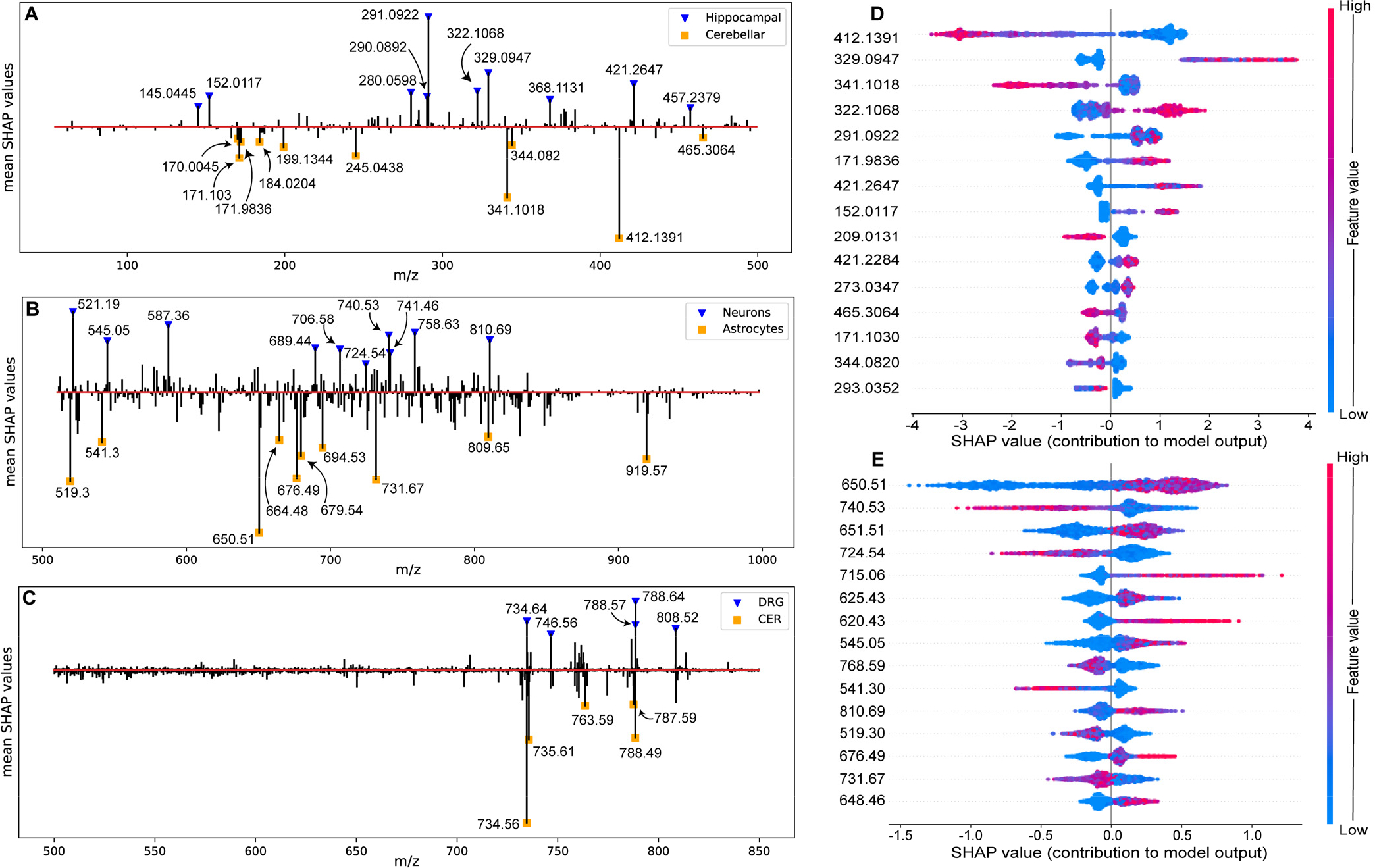
Averaged SHAP values plotted against m/z values for the (A) HIP_CER, (B) ICC, and (C) SIMS datasets. Density plots of the top contributing mass features determined by the mean absolute SHAP values for classifying (D) hippocampal cells (positive log probability) and cerebellar cells (negative log probability), and (E) neurons (positive log probability) and astrocytes (negative log probability).

From the top contributing features, we discovered multiple features that matched our expectations. For example, in the ICC dataset we found m/z 650.51 and m/z 651.51 to be the top two enriched features for predicting neurons (Figure 2E), which were reported as positive ions originating from ceramides in previous lipid research.⁴³ Ceramides are precursors of sphingolipids that are abundant on neuronal cell membranes and serve as potent regulators of brain homeostasis.² Another neuronal feature, m/z 810.69, matches [GalCer(d18:1/C24:1)+H]+,⁴⁴ a galactosylceramide considered crucial to maintaining brain health, especially for neuronal cells.⁴⁵ Lipid features such as m/z 724.54 ([PE(O-34:2)+Na]+, [PE(P-34:1)+Na]+), m/z 740.53 ([PE(34:4)+H]+) and m/z 768.59 ([PC(O-34:1)+Na]+, [PC(P-34:0)+Na]+, [PE(O-37:1)+Na]+, [PE(P-37:0)+Na]+) had large impacts for predicting that a cell was an astrocyte, consistent with previous studies.^14,44 Some contributing features could not be matched or identified (e.g., m/z 545.05 and m/z 715.06). The explained output of the models can be further investigated by focusing on the top m/z features determined by the SHAP values, and performing a subsequent analysis using tandem MS on the top / most interesting candidate ions to obtain structural information.

SHAP Values Reveal Model Decisions in Low-Dimensional Space.

PCA on the original dataset was largely affected by unwanted experimental variations (Figure 1), making it undesirable to perform “unsupervised” analyses. Instead, “supervision” was introduced by performing PCA on the feature contributions calculated by the SHAP values. Essentially, non-contributing features have zero or very small SHAP values, whereas contributing features relevant to classification tasks have larger SHAP values. The variations in the feature intensity only affect the outcome of PCA if they impact the model output.³¹ The first two PCs of the SHAP values show clustering on the GOI, demonstrating that the model learned group-specific knowledge (Figure 3A, Figure S5). The predicted log probability matched well with the clustering patterns of PCA (Figure 3B, Figure S5). There were ambiguous predictions where the model was not able to confidently differentiate GOI, such as in the ICC dataset where data points merged with decreasing predicted log probability for their associated groups. Merging of data points may happen when the spectral features of single cells from different GOI are similar, leading to suboptimal model performance.

Figure 3.

PCA performed on the SHAP values from the HIP_CER and ICC datasets, where (A) colors represent the true labels of the cell GOI (top: HIP_CER, bottom: ICC). (B) The corresponding PCA plots with the log odds (probability) as the color bar for HIP_CER (left) and ICC (right). Cells are separated in low-dimensional space by their GOI, indicating that feature contributions represented by SHAP values are group-specific. Each inset shows the SHAP values of a single-cell spectrum. SHAP PCA plots with visualization of mass feature normalized intensity to cell classification for the two datasets: (C) HIP_CER mass features m/z 412.1391 (left), m/z 322.1068 (middle), and m/z 341.1018 (right); and (D) ICC mass features m/z 650.51 (left), m/z 676.49 (middle) and m/z 768.59 (right).

Visualizing the normalized intensities of the contributing features on the “supervised” PCA plots helps us understand how predictions are made by the models. For the HIP_CER dataset, m/z 412.1391 and m/z 341.1018 were localized within cerebellar cells by model predictions (Figure 3C, left and right), whereas m/z 322.1068 prompted the model to make predictions toward hippocampal cells (Figure 3C, middle). Mass features of m/z 650.51 and m/z 676.49 in the ICC dataset were determined to contribute to predictions of cells as neurons (Figure 3D, left and middle), and m/z 768.59 contributed to predictions of astrocytes (Figure 3D, right). In the SIMS dataset, m/z 760.52 and m/z 788.57 contributed to DRG predictions and m/z 734.56 contributed to cerebellar cell predictions (Figure S5), consistent with our previous work.¹⁷ Similar visual inspections can be made for other mass features to enhance the model interpretations by looking at how peak intensities are localized with the model output.

Mean Absolute SHAP Values Serve as a Feature Selection Procedure.

Feature selection is a process in which features contributing to the prediction variables are selected, whereas those that do not contribute are deemed less relevant to the classification tasks. Several feature selection techniques were previously proposed: the rank-sum test was applied to identify and rank differentially expressed genes using genomic expression profiles;^37,46 model-dependent methods such as Recursive Feature Elimination SVM (RFE-SVM)⁴⁷ were used for gene selection for cancer classification, and a similar feature elimination procedure for the random forest.^39,48 The predictive power of the subsets of mass features was tested by selecting features based on the ranking of mean absolute SHAP values. Models were trained using incremental numbers of features, starting with the highest rank to the lowest. Performance metrics were computed for each model with a subset of features, and an optimal subset of features was chosen heuristically through the Elbow method, shown as dashed blue lines (Figure 4A, B). In order to test the strength of the selected predictors, we randomly sampled the same number of features (18 for the HIP_CER dataset and 45 for the ICC dataset) from all features 300 times and trained the models using those randomly sampled features. The distribution of AUC values from models trained on random features compared with the models trained on selected features (Figure 4C, D) suggests that ranking on mean absolute SHAP values is a way to select subsets of strong predictors for classifying cells from different GOI. Our technique essentially reduces a large number of m/z features to a much lower number specific to the defined GOI as candidates for further analysis and validation. The comprehensive list of SHAP-ranked features for the HIP_CER and the ICC datasets can be found in the Supporting Information (Tables S1, S2). Combining the information of top ranked features from three different ranking metrics (p-values, Gini, and mean absolute SHAP values) generated the lists of commonly shared features that can be more robust against false-positively identified features. Among the three ranking metrics, 9 features (m/z 284.2688, 290.0892, 291.0922, 322.1068, 377.2478, 378.2509, 412.1391, 421.2647, 483.2545) were commonly identified for the HIP_CER dataset (Figure 4E top), and 8 features (m/z 620.43, 648.46, 650.51, 651.51, 676.49, 724.54, 752.58, 758.63) for the ICC dataset (Figure 4E bottom).

Figure 4.

Model performance with an incremental number of features ranked by feature contributions for two datasets. (A) For the HIP_CER dataset, 18 features were selected with 0.98 AUC; (B) for the ICC dataset, 45 features were selected with 0.83 AUC. (C) AUC distribution of randomly selected features sampled 300 times with replacement for the HIP_CER dataset; (D) AUC distribution for the ICC dataset. (E) Venn diagrams of commonly identified features by three ranking metrics. Top: 9 features were shared for the HIP_CER dataset and bottom: 8 features were shared for the ICC dataset.

Classification of an Unlabeled Large Single-Cell Dataset Revealed GOI-Specific Knowledge.

Recently, single-cell MS analysis was applied to profile over 30,000 individual rodent cerebellar cells, demonstrating the application of high-throughput MS analysis to study cell-to-cell chemical differences in an unsupervised manner.⁹ Here we used our classification model trained on the ICC dataset to make predictions on that dataset; although the two datasets were acquired on different instruments and the cells were prepared from different animals, we expected that the unique mass features differentiating neurons and astrocytes would be preserved across samples. The input features from the mass spectra of the 30,000 cells were processed to align with peak features in the ICC dataset by taking the most intense peaks within a 0.1 m/z bin width. To interpret the model predictions, we then applied the SHAP framework to determine each feature’s contributions to the model output. The first two PCs of the SHAP values showed a divergence of feature contributions in predicting cells to be neuronal or astrocytic (Figure 5A). By selecting the top features based on their mean absolute SHAP values, we found consistency in the model explanations. For instance, m/z 545.05 and m/z 650.51 contributed most to predicting neurons (Figure 5C); m/z 724.54 and m/z 768.59 were determined to contribute to predicting astrocytes (Figure 5D, E), consistent with those shown for the ICC dataset and with our previous study¹⁴ (Figure S6). Neuron and astrocyte classifications explained by SHAP values revealed cell class-specific knowledge, and the top selected features were well-localized with model output. The ability to perform label-free canonical cell-type classification by supervised machine learning models previously trained on labeled cells needs further validation. Therefore, we aim to acquire more ICC-labeled single-cell mass spectra to test both the predictive powers and the limits of the model.

Figure 5.

(A) Model predictions of the 30,000 cells dataset were explained by SHAP values, visualized using PCA. The model was trained on the ICC dataset while predicting on unlabeled cells. Top selected features, (B, C) m/z 545.05 and m/z 650.51 for neurons, (D, E) m/z 724.54 and m/z 768.59 for astrocytes, were visualized on the SHAP PCA plot.

Limitations.

The input features for classification tasks of the ICC and HIP_CER datasets were extracted using peak picking algorithms. Peak picking reduces the dimensionality of data and aids in interpretability of features. However, peak picking may add bias to the analysis and allow valuable information to be omitted. Negative correlation exists between the probability of a peak picking algorithm not detecting a peak and the peak’s mean spectral intensity level (Figure S7), suggesting that peaks with lower signal intensities are less likely to be detected by peak picking algorithms, rather than being absent from the sample. An alternative solution to avoid the use of peak picking is through resampling and binning the entire spectra as the direct model input. Thus, preprocessing input data for the model requires additional considerations. The decision is whether to maximize the feature interpretability by performing peak-picking to generate a smaller list of mass features while potentially introducing biases, or to reduce biases by resampling the entire spectra, which contains a large set of features and compromises the interpretability.

CONCLUSIONS

We developed a workflow to classify single cells based on MALDI MS spectra through interpretable machine learning. This workflow was applied to datasets acquired across three different mass spectrometers (with vastly different performance specifications) for various GOI. Individual model predictions for single-cell spectra were locally explained by SHAP values for interpretation of a given mass feature’s contribution toward the model output. Computing the mean absolute SHAP values allowed us to select features that were important to the classification tasks, enabling global interpretations. Furthermore, PCA was applied on the SHAP values to demonstrate that the models learned group-specific knowledge and captured heterogeneous feature contributions among the single cells within a specific GOI. Future work will apply the classification workflow to a larger single-cell MALDI MS dataset that is sampled from multiple GOI.

REFERENCES

- (1).Hussain G; Wang J; Rasul A; Anwar H; Imran A; Qasim M; Zafar S; Kamran SKS; Razzaq A; Aziz N; Ahmad W; Shabbir A; Iqbal J; Baig SM; Sun T Role of Cholesterol and Sphingolipids in Brain Development and Neurological Diseases. Lipids Health Dis. 2019, 18, 26. [DOI] [PMC free article] [PubMed] [Google Scholar]
- (2).Olsen ASB; Færgeman NJ Sphingolipids: Membrane Microdomains in Brain Development, Function and Neurological Diseases. Open Biol. 2017, 7, pii: 170069. [DOI] [PMC free article] [PubMed] [Google Scholar]
- (3).Ng J; Papandreou A; Heales SJ; Kurian MA Monoamine Neurotransmitter Disorders—Clinical Advances and Future Perspectives. Nature Reviews Neurology 2015, 11, 567–584. [DOI] [PubMed] [Google Scholar]
- (4).Zenobi R Single-Cell Metabolomics: Analytical and Biological Perspectives. Science 2013, 342, 1243259. [DOI] [PubMed] [Google Scholar]
- (5).Neumann EK; Do TD; Comi TJ; Sweedler JV Exploring the Fundamental Structures of Life: Non-Targeted, Chemical Analysis of Single Cells and Subcellular Structures. Angew. Chem. Int. Ed 2019, 58, 9348–9364. [DOI] [PMC free article] [PubMed] [Google Scholar]
- (6).Lin Y; Trouillon R; Safina G; Ewing AG Chemical Analysis of Single Cells. Anal. Chem 2011, 83, 4369–4392. [DOI] [PMC free article] [PubMed] [Google Scholar]
- (7).Oomen PE; Aref MA; Kaya I; Phan NTN; Ewing AG Chemical Analysis of Single Cells. Anal. Chem 2019, 91, 588–621. [DOI] [PubMed] [Google Scholar]
- (8).Comi TJ; Neumann EK; Do TD; Sweedler JV MicroMS: A Python Platform for Image-Guided Mass Spectrometry Profiling. J. Am. Soc. Mass Spectrom 2017, 28, 1919–1928. [DOI] [PMC free article] [PubMed] [Google Scholar]
- (9).Neumann EK; Ellis JF; Triplett AE; Rubakhin SS; Sweedler JV Lipid Analysis of 30 000 Individual Rodent Cerebellar Cells Using High-Resolution Mass Spectrometry. Anal. Chem 2019, 91, 7871–7878. [DOI] [PMC free article] [PubMed] [Google Scholar]
- (10).Comi TJ; Do TD; Rubakhin SS; Sweedler JV Categorizing Cells on the Basis of Their Chemical Profiles: Progress in Single-Cell Mass Spectrometry. J. Am. Chem. Soc 2017, 139, 3920–3929. [DOI] [PMC free article] [PubMed] [Google Scholar]
- (11).Rappez L; Stadler M; Triana S; Phapale P; Heikenwalder M; Alexandrov T Spatial Single-Cell Profiling of Intracellular Metabolomes in Situ. bioRxiv 2019, 510222 10.1101/510222. [DOI] [Google Scholar]
- (12).Yao H; Zhao H; Zhao X; Pan X; Feng J; Xu F; Zhang S; Zhang X Label-Free Mass Cytometry for Unveiling Cellular Metabolic Heterogeneity. Anal. Chem 2019, 91, 9777–9783. [DOI] [PubMed] [Google Scholar]
- (13).Altelaar AFM; Klinkert I; Jalink K; de Lange RPJ; Adan RAH; Heeren RMA; Piersma SR Gold-Enhanced Biomolecular Surface Imaging of Cells and Tissue by SIMS and MALDI Mass Spectrometry. Anal. Chem 2006, 78, 734–742. [DOI] [PubMed] [Google Scholar]
- (14).Neumann EK; Comi TJ; Rubakhin SS; Sweedler JV Lipid Heterogeneity between Astrocytes and Neurons Revealed by Single-Cell MALDI-MS Combined with Immunocytochemical Classification. Angew. Chem. Int. Ed 2019, 58, 5910–5914. [DOI] [PMC free article] [PubMed] [Google Scholar]
- (15).Hwang B; Lee JH; Bang D Single-Cell RNA Sequencing Technologies and Bioinformatics Pipelines. Exp. Mol. Med 2018, 50, 1–14. [DOI] [PMC free article] [PubMed] [Google Scholar]
- (16).Shekhar K; Lapan SW; Whitney IE; Tran NM; Macosko EZ; Kowalczyk M; Adiconis X; Levin JZ; Nemesh J; Goldman M; McCarroll SA; Cepko CL; Regev A; Sanes JR Comprehensive Classification of Retinal Bipolar Neurons by Single-Cell Transcriptomics. Cell 2016, 166, 1308–1323.e30. [DOI] [PMC free article] [PubMed] [Google Scholar]
- (17).Do TD; Comi TJ; Dunham SJB; Rubakhin SS; Sweedler JV Single Cell Profiling Using Ionic Liquid Matrix-Enhanced Secondary Ion Mass Spectrometry for Neuronal Cell Type Differentiation. Anal. Chem 2017, 89, 3078–3086. [DOI] [PMC free article] [PubMed] [Google Scholar]
- (18).Verbeeck N; Caprioli RM; Plas RV de. Unsupervised Machine Learning for Exploratory Data Analysis in Imaging Mass Spectrometry. Mass Spectrometry Reviews 2020, 39, 245–291. [DOI] [PMC free article] [PubMed] [Google Scholar]
- (19).Statistical Analysis of Proteomics, Metabolomics, and Lipidomics Data Using Mass Spectrometry; Datta S, Mertens BJA, Eds.; Frontiers in Probability and the Statistical Sciences; Springer International Publishing, 2017. [Google Scholar]
- (20).Tarca AL; Carey VJ; Chen X; Romero R; Drăghici S Machine Learning and Its Applications to Biology. PLOS Comput. Biol 2007, 3, e116. [DOI] [PMC free article] [PubMed] [Google Scholar]
- (21).Camacho DM; Collins KM; Powers RK; Costello JC; Collins JJ Next-Generation Machine Learning for Biological Networks. Cell 2018, 173, 1581–1592. [DOI] [PubMed] [Google Scholar]
- (22).Caicedo JC; Cooper S; Heigwer F; Warchal S; Qiu P; Molnar C; Vasilevich AS; Barry JD; Bansal HS; Kraus O; Wawer M; Paavolainen L; Herrmann MD; Rohban M; Hung J; Hennig H; Concannon J; Smith I; Clemons PA; Singh S; Rees P; Horvath P; Linington RG; Carpenter AE Data-Analysis Strategies for Image-Based Cell Profiling. Nat. Methods 2017, 14, 849–863. [DOI] [PMC free article] [PubMed] [Google Scholar]
- (23).Belthangady C; Royer LA Applications, Promises, and Pitfalls of Deep Learning for Fluorescence Image Reconstruction. Nat. Methods 2019, 16, 1215–1225. [DOI] [PubMed] [Google Scholar]
- (24).López-Fernández H; Santos HM; Capelo JL; Fdez-Riverola F; Glez-Peña D; Reboiro-Jato M Mass-Up: An All-in-One Open Software Application for MALDI-TOF Mass Spectrometry Knowledge Discovery. BMC Bioinformatics 2015, 16, 318. [DOI] [PMC free article] [PubMed] [Google Scholar]
- (25).Behrmann J; Etmann C; Boskamp T; Casadonte R; Kriegsmann J; Maaβ P Deep Learning for Tumor Classification in Imaging Mass Spectrometry. Bioinformatics 2018, 34, 1215–1223. [DOI] [PubMed] [Google Scholar]
- (26).Dominguez DC; Lopes R; Torres ML Proteomics: Clinical Applications. Clin. Lab. Sci. J. Am. Soc. Med. Technol 2007, 20, 245–248. [PubMed] [Google Scholar]
- (27).Zhou Z; Alvarez D; Milla C; Zare RN Proof of Concept for Identifying Cystic Fibrosis from Perspiration Samples. Proc. Natl. Acad. Sci 2019, 116, 24408–24412. [DOI] [PMC free article] [PubMed] [Google Scholar]
- (28).Zhou Z; Zare RN Personal Information from Latent Fingerprints Using Desorption Electrospray Ionization Mass Spectrometry and Machine Learning. Anal. Chem 2017, 89, 1369–1372. [DOI] [PubMed] [Google Scholar]
- (29).Hanselmann M; Köthe U; Kirchner M; Renard BY; Amstalden ER; Glunde K; Heeren RMA; Hamprecht FA Toward Digital Staining Using Imaging Mass Spectrometry and Random Forests. J. Proteome Res 2009, 8, 3558–3567. [DOI] [PMC free article] [PubMed] [Google Scholar]
- (30).Rudin C Stop Explaining Black Box Machine Learning Models for High Stakes Decisions and Use Interpretable Models Instead. Nat. Mach. Intell 2019, 1, 206–215. [DOI] [PMC free article] [PubMed] [Google Scholar]
- (31).Lundberg SM; Erion GG; Lee S-I Consistent Individualized Feature Attribution for Tree Ensembles. ArXiv180203888 Cs Stat 2019. [Google Scholar]
- (32).Lanni EJ; Dunham SJB; Nemes P; Rubakhin SS; Sweedler JV Biomolecular Imaging with a C60-SIMS/MALDI Dual Ion Source Hybrid Mass Spectrometer: Instrumentation, Matrix Enhancement, and Single Cell Analysis. J. Am. Soc. Mass Spectrom 2014, 25, 1897–1907. [DOI] [PubMed] [Google Scholar]
- (33).Chen T; Guestrin C XGBoost: A Scalable Tree Boosting System. Proc. 22nd ACM SIGKDD Int. Conf. Knowl. Discov. Data Min. - KDD 16 2016, 785–794. [Google Scholar]
- (34).Pedregosa F; Varoquaux G; Gramfort A; Michel V; Thirion B; Grisel O; Blondel M; Prettenhofer P; Weiss R; Dubourg V; Vanderplas J; Passos A; Cournapeau D; Brucher M; Perrot M; Duchesnay É Scikit-Learn: Machine Learning in Python. J. Mach. Learn. Res 2011, 12, 2825–2830. [Google Scholar]
- (35).Nembrini S; König IR; Wright MN The Revival of the Gini Importance? Bioinformatics 2018, 34, 3711–3718. [DOI] [PMC free article] [PubMed] [Google Scholar]
- (36).Lundberg SM; Lee S-I A Unified Approach to Interpreting Model Predictions In Advances in Neural Information Processing Systems 30; Guyon I, Luxburg UV, Bengio S, Wallach H, Fergus R, Vishwanathan S, Garnett R, Eds.; Curran Associates, Inc., 2017; pp 4765–4774. [Google Scholar]
- (37).Troyanskaya OG; Garber ME; Brown PO; Botstein D; Altman RB Nonparametric Methods for Identifying Differentially Expressed Genes in Microarray Data. Bioinformatics 2002, 18, 1454–1461. [DOI] [PubMed] [Google Scholar]
- (38).Cole MB; Risso D; Wagner A; DeTomaso D; Ngai J; Purdom E; Dudoit S; Yosef N Performance Assessment and Selection of Normalization Procedures for Single-Cell RNA-Seq. Cell Syst. 2019, 8, 315–328.e8. [DOI] [PMC free article] [PubMed] [Google Scholar]
- (39).Díaz-Uriarte R; Alvarez de Andrés S Gene Selection and Classification of Microarray Data Using Random Forest. BMC Bioinformatics 2006, 7, 3. [DOI] [PMC free article] [PubMed] [Google Scholar]
- (40).Hu Y; Hase T; Li HP; Prabhakar S; Kitano H; Ng SK; Ghosh S; Wee LJK A Machine Learning Approach for the Identification of Key Markers Involved in Brain Development from Single-Cell Transcriptomic Data. BMC Genomics 2016, 17, 1025. [DOI] [PMC free article] [PubMed] [Google Scholar]
- (41).Chen X; Ishwaran H Random Forests for Genomic Data Analysis. Genomics 2012, 99, 323–329. [DOI] [PMC free article] [PubMed] [Google Scholar]
- (42).Louppe G; Wehenkel L; Sutera A; Geurts P Understanding Variable Importances in Forests of Randomized Trees In Advances in Neural Information Processing Systems 26; Burges CJC, Bottou L, Welling M, Ghahramani Z, Weinberger KQ, Eds.; Curran Associates, Inc., 2013; pp 431–439. [Google Scholar]
- (43).Colsch B; Afonso C; Popa I; Portoukalian J; Fournier F; Tabet J-C; Baumann N Characterization of the Ceramide Moieties of Sphingoglycolipids from Mouse Brain by ESI-MS/MS: Identification of Ceramides Containing Sphingadienine. J. Lipid Res 2004, 45, 281–286. [DOI] [PubMed] [Google Scholar]
- (44).Soltwisch J; Kettling H; Vens-Cappell S; Wiegelmann M; Müthing J; Dreisewerd K Mass Spectrometry Imaging with Laser-Induced Postionization. Science 2015, 348, 211–215. [DOI] [PubMed] [Google Scholar]
- (45).Mencarelli C; Martinez–Martinez P Ceramide Function in the Brain: When a Slight Tilt Is Enough. Cell. Mol. Life Sci 2013, 70, 181–203. [DOI] [PMC free article] [PubMed] [Google Scholar]
- (46).Thomas JG; Olson JM; Tapscott SJ; Zhao LP An Efficient and Robust Statistical Modeling Approach to Discover Differentially Expressed Genes Using Genomic Expression Profiles. Genome Res. 2001, 11, 1227–1236. [DOI] [PMC free article] [PubMed] [Google Scholar]
- (47).Guyon I; Weston J; Barnhill S; Vapnik V Gene Selection for Cancer Classification Using Support Vector Machines. Mach. Learn 2002, 46, 389–422. [Google Scholar]
- (48).Darst BF; Malecki KC; Engelman CD Using Recursive Feature Elimination in Random Forest to Account for Correlated Variables in High-dimensional Data. BMC Genet. 2018, 19, 65. [DOI] [PMC free article] [PubMed] [Google Scholar]
Associated Data
This section collects any data citations, data availability statements, or supplementary materials included in this article.