

Abstract
Marine cloud brightening (MCB) is proposed to offset global warming by emitting sea salt aerosols to the tropical marine boundary layer, which increases aerosol and cloud albedo. Sea salt aerosol is the main source of tropospheric reactive chlorine (Cly) and bromine (Bry). The effects of additional sea salt on atmospheric chemistry have not been explored. We simulate sea salt aerosol injections for MCB under two scenarios (212–569 Tg/a) in the GEOS‐Chem global chemical transport model, only considering their impacts as a halogen source. Globally, tropospheric Cly and Bry increase (20–40%), leading to decreased ozone (−3 to −6%). Consequently, OH decreases (−3 to −5%), which increases the methane lifetime (3–6%). Our results suggest that the chemistry of the additional sea salt leads to minor total radiative forcing compared to that of the sea salt aerosol itself (~2%) but may have potential implications for surface ozone pollution in tropical coastal regions.
Keywords: geoengineering, atmospheric chemistry, sea salt aerosols, reactive halogens, marine cloud brightening
Key Points
Sea salt aerosol emissions for Marine Cloud Brightening geoengineering are implemented in a global chemical transport model
This leads to changes in global tropospheric Bry and Cly (+20 to 40%), ozone (−3 to −6%), OH (−2 to −4%), and methane lifetime (+3 to 6%)
Chemistry of the added sea salt leads to minor total radiative forcing (−20 to −50 mW/m2) but may have implications for ozone pollution
1. Introduction
Marine cloud brightening (MCB) is a geoengineering strategy to offset climate warming arising from increases in anthropogenic greenhouse gases first proposed in Latham (1990, 2002). This method would spray sea salt aerosols in the tropical marine boundary layer (MBL) where stratocumulus clouds have a large radiative impact (Alterskjær et al., 2012; Jones & Haywood, 2012). Increasing the flux of accumulation‐mode sea salt aerosols into the MBL is expected to cool the climate by reflecting sunlight directly (Partanen et al., 2012) and increasing cloud reflectivity by increasing cloud condensation nuclei concentrations and decreasing the radius of cloud droplets (Latham, 1990).
Several studies have investigated radiative forcing (RF) from MCB following the Geoengineering Model Intercomparison Project (GeoMIP) framework of sea salt aerosol emissions throughout the tropical MBL (Kravitz et al., 2013; Alterskjaer et al., 2013; Ahlm et al., 2017). Others determine limited, optimized areas of sea salt emissions for MCB, which depend on the model or data used and implementation strategies (e.g., Jones et al., 2009; Partanen et al., 2012; Salter et al., 2008). Kravitz et al. (2013) suggest that an accumulation‐mode sea salt aerosol flux of 212 Tg/a achieves a radiative cooling of −2 W/m2. Alterskjaer et al. (2013) find that a flux of 266–569 Tg/a, dependent on the model used, is required to maintain global mean temperatures from 2020 CE through 2060–2070 CE under the RCP4.5 emissions scenario. Ahlm et al. (2017) suggest that in a tropics‐wide emissions framework the direct cooling from the scattering of radiation by sea salt aerosols is nearly as effective as the indirect cooling from increased cloud albedo.
Halogens strongly affect the chemistry of the troposphere, including that of pollutants like mercury and greenhouse gases like methane and ozone (Simpson et al., 2015). Sea salt aerosols are thought to be the main source of reactive bromine (Bry) and reactive chlorine (Cly) to the MBL (Chen et al., 2017; Schmidt et al., 2016; Sherwen, Schmidt, et al., 2016). Reactive halogens are released from sea salt aerosols via heterogeneous reactions (e.g., HOBr + Br− + H+ ➔ Br2 + H2O) (Fan & Jacob, 1992; Vogt et al., 1996). The main source of reactive iodine (Iy) is thought to be release from the sea surface from the reaction of ocean iodide with ozone following ozone dry deposition (Carptenter et al., 2013; Sherwen, Evans, et al., 2016). Reactive halogen chemistry has implications for the oxidative capacity of the atmosphere, as it is a sink for ozone and nitrogen oxides (NOx = NO + NO2) (Simpson et al., 2015). Implementation of reactive halogen chemistry into a global model of tropospheric chemistry resulted in decreases in global mean concentrations of ozone (−18.6%) and OH (−8.2%), leading to a 10.8% increase in methane lifetime (Sherwen, Schmidt, et al., 2016). This is consistent with observations of surface ozone destruction coinciding with high concentrations of reactive halogens (e.g., Barrie et al., 1988; Read et al., 2008). Br atom is also a major oxidant of atmospheric mercury (e.g., Horowitz et al., 2017).
Here we explore, for the first time, the atmospheric chemistry implications of sea salt aerosol injections for MCB. We focus on the impacts of this additional tropical sea salt aerosol source on tropospheric oxidants, sulfate‐nitrate‐ammonium aerosols, and methane via changes to reactive halogen production. We examine the air quality and RF implications of these chemical effects, focusing on tropospheric ozone abundance, methane lifetime, and heterogeneous aerosol production.
2. Methods
We use the GEOS‐Chem global 3D chemical transport model from Wang et al. (2019) including chlorine chemistry, built off of the reference version 11‐02d. Simulations are performed at 4° × 5° horizontal resolution with 47 vertical layers. The model is driven by assimilated offline meteorology, including cloud parameters, from the Goddard Earth Observing System Forward Processing product of the NASA Global Modeling and Assimilation Office. Simulations are performed for the arbitrary year 2014 following 6 months of initialization (June–December 2013).
The model contains detailed, coupled HOx‐NOx‐VOC‐ozone‐halogen‐aerosol tropospheric chemistry (http://geos-chem.org). In addition to Wang et al. (2019), other recent updates to reactive halogen (Br, Cl, and I) chemistry are described in Sherwen, Schmidt, et al. (2016) and Chen et al. (2017). Sea salt aerosol emissions from the open ocean are dependent on wind speed and sea surface temperature, described in detail in Jaeglé et al. (2011) including evaluation against observed in situ concentrations and Moderate Resolution Imaging Spectroradiometer and Aerosol Robotic Network aerosol optical depth. Sea salt aerosol represents the largest source of reactive bromine and chlorine in the model (Chen et al., 2017; Wang et al., 2019). Carbonaceous aerosol includes black carbon (Wang et al., 2014) and organic aerosol following the “simple” SOA scheme (fixed‐yield, direct, and irreversible formation) (Kim et al., 2015). Sulfate aerosol forms by gas‐phase reaction of SO2 with OH, in cloud droplets via oxidation of S (IV) (= SO2•H2O + HSO3 − + SO3 2−) by H2O2, ozone, and HOBr (Chen et al., 2017), and on the surface of alkaline sea salt aerosol via oxidation by ozone (Alexander et al., 2005). Inorganic nitrate aerosol is formed through hydrolysis of NO2, NO3, halogen nitrates, organic nitrates, and N2O5 on aerosol surfaces; reaction of NO2 with OH and HO2; reaction of N2O5 with particle chloride; and reaction of NO3 with hydrocarbons (Schmidt et al., 2016b). Aerosols interact with gas‐phase chemistry through the effect of aerosol extinction on photolysis rates (Martin et al., 2003), heterogeneous chemistry (Jacob, 2000), and gas‐aerosol partitioning of sulfate‐nitrate‐ammonium aerosols as calculated in the ISORROPIA‐II aerosol thermodynamic module (Fountoukis & Nenes, 2007). The model contains wet and dry deposition schemes for both gas and aerosol species (Amos et al., 2012; Liu et al., 2001; Wang et al., 1998; Zhang et al., 2001). Photolysis is calculated using the FAST‐JX module (Bian & Prather, 2002) as described in Mao et al. (2010) and Eastham et al. (2014). All aerosols in GEOS‐Chem are treated as externally mixed.
We perform three model simulations for this study. All simulations include “sea salt dehalogenation” or heterogeneous chemical reactions on the surface of sea salt aerosols that convert halides (e.g., Br−) to their reactive form (e.g., BrO). All are forced with the same specified assimilated meteorology (including cloud properties), eliminating meteorological variability that could obscure the effects of sea salt aerosol chemistry. The meteorology does not respond to changing atmospheric composition. “Standard” runs do not include the additional MCB sea salt flux. We implement two MCB sea salt aerosol emission scenarios, “MCBlow” and “MCBhigh”. These sample near the low and high end of emissions employed in climate modeling studies throughout the tropics to offset RF from the Representative Concentration Pathway (RCP) 4.5 scenario. The Kravitz et al. (2013) G4 sea salt modeling study employed a flux of sea salt of 212 Tg/a to offset 2 W/m2 effective RF. We replicate this in MCBlow by adding a spatially and temporally uniform flux of sea salt (3.0 × 10⁻¹² kg·m−2·s−1) to the MBL over the tropical oceans (30°N to 30°S). Another modeling study (G3‐SSCE) held the RF at the top of the atmosphere at 2020 levels until 2070 by continuously increasing the flux of sea salt into the MBL (Alterskjaer et al., 2013). We implement the maximum flux found from 2060 to 2070 (569 Tg/a) by uniformly emitting 8.0 × 10⁻¹² kg·m−2·s−1 of sea salt over the tropical oceans for MCBhigh. Sea salt aerosol in GEOS‐Chem is transported in two tracers: accumulation mode (r dry = 0.01–0.5 μm) and coarse mode (r dry = 0.5–8 μm). In both MCB scenarios, additional sea salt is emitted as accumulation‐mode particles. The assumed size distribution for the optical properties of accumulation‐mode sea salt aerosol in GEOS‐Chem is a dry geometric mean radius of 0.085 μm and a geometric standard deviation of 1.5 μm (Jaeglé et al., 2011). This is similar to the distributions in Kravitz et al. (2013) and Alterskjaer et al. (2013) but may be larger than the most efficient particle size for MCB (0.03–0.1 μm dry diameter; Connolly et al., 2014). Hygroscopic growth as a function of local relative humidity follows Gerber (1985) (Jaeglé et al., 2011) and may be overestimated (Zieger et al., 2017).
We calculate the RF of MCB from greenhouse gases and aerosols as the difference between radiative effects in simulations with MCB and the Standard model. Meteorological conditions are identical in all simulations, so the RF is entirely attributed to composition changes. RF is calculated at the tropopause with stratospheric temperature adjustment. For methane, tropospheric ozone, and aerosol‐radiation interactions of reflective aerosols, effective radiative forcing (ERF) is nearly identical to RF (Myhre et al., 2013). In GEOS‐Chem, direct radiative effects of tropospheric aerosols are computed instantaneously at the top of the atmosphere in the RRTMG module (Heald et al., 2014). The IPCC (2007) report found that stratospheric temperature adjustment has little effect on the RF for tropospheric aerosols and hence the instantaneous top‐of‐atmosphere RF is an appropriate substitution. For ozone, we calculate the stratospheric temperature adjustment and RF from monthly mean ozone fields simulated in GEOS‐Chem using the method of Conley et al. (2013). Methane concentrations are not simulated directly. We calculate the change in steady state methane concentrations based on the change in simulated methane lifetime and feedback of methane on its own loss rate following Holmes et al. (2013) and Holmes (2018). The RF of the change in methane, including its indirect RF through effects on stratospheric water vapor and ozone production, is calculated following Intergovernmental Panel on Climate Change (IPCC) methodology (Myhre et al., 2013). For additional information, see the supporting information.
3. Results
3.1. Impacts of MCB Sea Salt Aerosol Emissions on Halogens, Oxidants, and Aerosols
In the Standard model, annual emissions of accumulation‐mode sea salt aerosol are 51 Tg/a, with coarse mode emissions of 3,090 Tg/a, resulting in global annual‐mean tropospheric burdens of 320 and 3,500 Gg, respectively. Coarse mode sea salt remains unchanged in our study. In the MCB scenarios, the global annual‐mean tropospheric burden of accumulation‐mode sea salt aerosol is increased by a factor of 4.2–9.7 (MCBlow‐MCBhigh) over the Standard. Over the tropical oceans, surface as a factor of 31–83 (MCBlow‐MCBhigh) higher (see Figure S1 in the supporting information). This impacts concentrations of reactive halogens and oxidants OH and ozone (Table 1 and Figures 1 and 2), with the largest changes near the surface in the tropics where the MCB source of sea salt aerosol is emitted. We define reactive halogen families (Bry, Cly, Iy) as in Sherwen, Schmidt, et al. (2016) (see Table S1).
Table 1.
Global, Annual‐Mean Tropospheric Burden (Percent Change Relative to “Standard” Simulation)
| Standard | MCBlow | MCBhigh | Unit | |
|---|---|---|---|---|
| Bry | 36.9 | 44.5 (+21%) | 52.3 (+42%) | Gg |
| Cly | 356.4 | 432.0 (+20%) | 489.0 (+35%) | Gg |
| Iy | 11.7 | 11.1 (−5%) | 9.7 (−17%) | Gg |
| O3 | 319.0 | 309.2 (−3%) | 300.3 (−6%) | Tg |
| OH | 236 | 232 (−2%) | 228 (−4%) | Mg |
| Cl | 249.0 | 319.7 (+28%) | 395.2 (+59%) | kg |
Note. OH is an air mass‐weighted concentration.
Figure 1.

Standard, annual‐mean surface concentrations (left column) and relative difference for MCBlow (middle column) and MCBhigh (right column) relative to Standard of Bry (top row) and Cly (bottom row).
Figure 2.
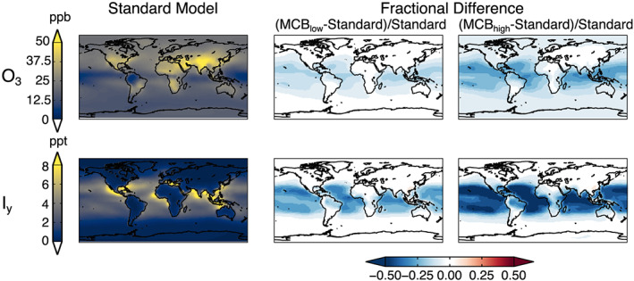
Same as Figure 1 but for surface ozone (top row) and Iy (bottom row).
The global tropospheric Bry burden increases by 21% and 42% for MCBlow and MCBhigh, respectively (Table 1), relative to Standard. Figure 1 (top row) shows the spatial distribution of the differences in surface Bry concentrations for the MCBlow and MCBhigh scenarios, relative to Standard. The short lifetime of Bry limits its changes to the tropics (Sherwen, Schmidt, et al., 2016). Both MCB scenarios show increases in surface Bry concentrations of up to a factor of 2.9 (MCBlow) to 6.1 (MCBhigh) over the tropical oceans, with smaller decreases over the Southern Ocean of <20% and over the northwestern North Pacific and northern North Atlantic (<5%).
The global tropospheric Cly burden increases by 20% and 35% for MCBlow and MCBhigh, respectively, relative to Standard (Table 1). The largest absolute changes in surface Cly concentrations (not shown) occur in outflow regions of South, East, and Southeast Asia where concentrations of acid gases such as SO2 and HNO3 are high. These acids are needed to liberate sea salt Cl− as HCl via acid displacement, which is the largest source of Cly (Wang et al., 2019). The bottom row of Figure 1 shows the spatial distribution of the relative differences in surface Cly concentrations for MCBlow and MCBhigh scenarios to the Standard. Similar to surface Bry, surface Cly increases over the tropical oceans by up to a factor of 4.1–6.3 (MCBlow‐MCBhigh) with smaller decreases over the Southern Ocean and Northern Europe of <4% to <8% (MCBlow to MCBhigh).
Increases in Bry and Cly lead to decreases of 3–6% in the global tropospheric ozone burden (Table 1). Reductions in ozone result primarily from its direct reaction with halogens to form species such as BrO and ClO. Reactive halogens also act as a sink for NOx through the formation and hydrolysis of halogen nitrates, resulting in a reduction of global tropospheric NOx of −0.6 to −1.6%. Lower NOx concentrations result in a decrease in the ozone production rate (Schmidt et al., 2016; Sherwen, Schmidt, et al., 2016). Although the largest declines in ozone occur over the tropics, the change in surface ozone concentrations is more spatially widespread due to its longer lifetime compared to Bry and Cly (Figure 2, top row). Decreases in surface ozone concentrations are as high as 21–34% in the tropics, with mean reductions of 1.8 ppb (MCBlow) and 3.5 ppb (MCBhigh).
The main source of reactive iodine (Iy) is not from sea salt aerosol but from deposition of ozone to the ocean surface (Sherwen, Evans, et al., 2016). Thus, the combination of decreased surface ozone and increased aerosol surface area to which Iy can be lost leads to declines in the tropospheric Iy burden of −5% and −17% for MCBlow and MCBhigh, respectively, relative to Standard (Table 1). Decreases in Iy concentrations are highest over the tropical oceans where ozone decreases are also largest (Figure 2, bottom row). Limited areas over land in East and equatorial Asia and the northeast United States experience increases in surface Iy of up to 15% (MCBlow) and 8% (MCBhigh).
Table 1 shows the global tropospheric burden of OH in each model simulation in Mg. The additional MCB flux of sea salt aerosol results in decreases in global tropospheric OH burden of −2% and −4% for MCBlow and MCBhigh, respectively, relative to the Standard simulation. Consistent with Sherwen, Schmidt, et al. (2016) and Wang et al. (2019), the additional source of reactive halogens results in decreases in OH due to the loss of ozone, since ozone is the primary source of OH globally (Sherwen, Schmidt, et al., 2016). As the OH decrease is concentrated in the warmer‐than‐average tropical MBL and lower troposphere, the change in methane lifetime against loss via tropospheric OH alone is relatively larger (4% and 8% increase in MCBlow and MCBhigh) (see Text S1 and Table S2).
Given the changes in atmospheric oxidants and sea salt aerosol, the global annual‐mean tropospheric burden of sulfate‐nitrate‐ammonium (SNA) increases by 1.9% (MCBlow) to 6.5% (MCBhigh). In the tropics, we find surface concentrations increase by up to a factor of 1.6 to 2.4 (MCBlow to MCBhigh) (Figure S2). The overall change in surface SNA is dominated by increases in nitrate driven by hydrolysis of halogen nitrates.
We find that changes in the tropospheric burdens of Cly, Bry, ozone, and OH scale sublinearly with increasing tropical sea salt aerosol emissions. The Iy burden changes superlinearly potentially due to the combination of a decreased source and increased sink to aerosol as discussed in this section. Increases in SNA are also superlinear.
3.2. Radiative Forcing of MCB Including Atmospheric Chemistry Impacts
First, we discuss the RF of sea salt aerosols for MCB in GEOS‐Chem relative to previous studies to put in context our estimates of the RF from atmospheric chemistry effects presented in the next paragraph. We find that the global, annual‐mean direct RF of the additional sea salt aerosol is −1.03 to −2.67 W/m2 (MCBlow to MCBhigh). The direct effect is also known as aerosol‐radiation interactions. Kravitz et al. (2013), on which our MCBlow experiment is based, estimated that 212 Tg/a sea salt would result in the desired −2.0 W/m2 total ERF using the HadGEM2‐ES model (with assumed median radius 0.1 and 1.9 μm geometric standard deviation for optical properties) (Bellouin et al., 2011). They found in a different simulation with 100 Tg/a sea salt aerosol emitted that 64% of total ERF from MCB is due to the direct effect. Assuming this division holds, −2.0 W/m2 total ERF would result in approximately −1.27 W/m2 from the direct effect alone in their model, which is slightly larger than our estimate of direct effect RF. Some of the difference may be because ERF includes short‐term adjustments in the land surface and troposphere, such that the IPCC AR5 found ERF was slightly higher than RF for aerosol‐radiation interactions for total tropospheric aerosol (Myhre et al., 2013). The IPSL‐CM5A model in Alterskjaer et al. (2013), which required the largest emissions of sea salt aerosol to offset RF from greenhouse gases and on which our MCBhigh experiment is based, led to a global mean total shortwave RF of −2.4 W/m2. This is smaller than our estimate of the direct effect alone in MCBhigh (−2.67 W/m2), which may be because the emitted sea salt particles in Alterskjaer et al. (2013) were larger in size (mode radius of geometric mean 0.13 μm with 1.59 μm geometric standard deviation vs geometric mean 0.085 μm with 1.5 μm geometric standard deviation in our study).
Table 2 shows the RF from the atmospheric chemistry impacts of MCB sea salt aerosol emissions in our two model experiments. Changes in the chemical production of other aerosol species (see section 3.1. and Figure S2) result in an additional direct RF of −0.022 to −0.064 W/m2 (MCBlow to MCBhigh). Declines in tropospheric ozone abundances from MCB sea salt chemistry result in a negative RF of −0.037 to −0.072 W/m2 (MCBlow to MCBhigh). For reference, the RF due to ozone depletion from CFCs and their substitutes is −0.15 W/m2 in year 2011 relative to 1750 (Myhre et al., 2013). Changes to reactive halogens are limited to the troposphere and do not influence stratospheric ozone (Figures S3 and S4).
Table 2.
Radiative Forcing by Components From the Atmospheric Chemistry of MCB Sea Salt Aerosol Emissions (mW/m2)
| MCBlow | MCBhigh | |
|---|---|---|
| Aerosol‐radiation interactions, sulfate‐nitrate‐ammonium aerosols | −21.8 | −64.0 |
| Direct O3 | −37.7 ± 4.5 | −71.9 ± 8.6 |
| CH4 | 24.1 ± 2.7 | 49.4 ± 5.4 |
| Indirect O3 from CH4 | 12.1 ± 7.3 | 24.7 ± 14.9 |
| Stratospheric H2O from CH4 | 3.6 ± 1.7 | 7.4 ± 3.6 |
| Total | −19.7 ± 9.3 | −54.3 ± 18.8 |
Note. Radiative forcing is calculated at the tropopause with stratospheric temperature adjustment. Ranges represent one‐sigma uncertainty in the radiative forcing efficiencies (see Text S1), not scenario uncertainty.
While we do not simulate changing methane concentrations directly (see section 2. and Text S1), we calculate the net change in methane lifetime from decreased OH and increased Cl concentrations and find that it increases from 8.54 years in the Standard to 8.77–9.01 years (MCBlow‐MCBhigh) (see Table S2). The relative change is at least as large as interannual variability in methane lifetime over the last two decades (<2% to ~5%; e.g., Montzka et al., 2011; Holmes et al., 2013; Rigby et al., 2017; Turner et al., 2017), but the effects would be additive. The RF due to the associated increase in methane concentrations alone is 0.024–0.049 W/m2 (MCBlow to MCBhigh) or an additional 5% to 10% of its estimated RF for year 2011 relative to 1750 (0.48 W/m2; Myhre et al., 2013). Increases in methane would serve to increase tropospheric ozone and stratospheric water vapor, leading to additional positive RF (see Table 2). Combining the methane‐mediated changes in ozone with the directly simulated ozone changes, we estimate then that the net RF of ozone from MCB is −0.025 to −0.047 W/m2 (MCBlow‐MCBhigh), which would decrease the present‐day RF of ozone (0.35 W/m2; Myhre et al., 2013) by 7.2% to 13.5%, respectively.
The net global mean RF due to the atmospheric chemistry impacts of MCB is small (−0.020 to −0.054 W/m2 for MCBlow to MCBhigh) relative to the forcing from aerosol‐radiation interactions of the additional sea salt alone (−1.03 to −2.67 W/m2). At the same time, the forcings from individual agents have different geographic distributions, which produce regional variability. For example, longer‐lived ozone (Figure 2) and methane are more well mixed than the shorter‐lived sea salt and sulfate‐nitrate‐ammonium aerosols, whose impacts are limited to the tropics (Figures S1 and S2).
3.3. Uncertainties
This study used a global chemical transport model driven by present‐day assimilated meteorology to provide a first look at the potential impacts of additional sea salt for MCB on atmospheric chemistry and the implications for RF. As such, chemistry‐climate change feedbacks are not represented. A major uncertainty in this approach is that the additional sea salt aerosol does not impact cloud properties. Heterogeneous recycling of bromine in clouds and aerosols is a major driver of tropospheric Bry (e.g., Chen et al., 2017; Parrella et al., 2012). Increases in cloudiness and cloud droplet surface area from MCB would likely increase this recycling, potentially leading to greater increases in reactive halogens and changes to ozone and methane than presented here. On a global scale, most sulfate formation occurs in cloud droplets and is impacted by cloud pH and cloud drop size (e.g., Alexander et al., 2012), both of which may also be affected by MCB sea salt aerosol emissions. Increased cloud optical depth would also affect photolysis rates, with decreases below cloud and increases above the cloud top. Sea salt injections for MCB may also affect precipitation and boundary layer dynamics (e.g., Wang et al., 2011; Wang & Feingold, 2009), which would impact aerosol transport and scavenging. Conversely, background meteorological conditions may impact how effectively sea salt aerosol influences cloud formation (e.g., Jones & Haywood, 2012). Finally, the size of geoengineered sea salt particles affects their ability to impact clouds and produce a cooling effect, as discussed in Connolly et al. (2014), who find an optimal size range of 30–100 nm median dry diameter. A different size distribution of sea salt aerosol particles specifically emitted for MCB, which will depend on technological development, would also affect the rates of heterogeneous reactions that depend on aerosol surface area. This could be explored in future studies.
4. Conclusions
Marine Cloud Brightening (MCB) is a geoengineering technique where sea salt aerosols are released in the tropical marine boundary layer to increase cloud albedo and scatter light, offsetting the radiative forcing (RF) from greenhouse gases. Sea salt aerosol is the largest source of tropospheric reactive halogens, and their atmospheric chemistry and RF impacts have not yet been quantified in the context of MCB. Here we use the GEOS‐Chem chemical transport model to simulate these effects. Accumulation‐mode sea salt aerosol is emitted continuously in the tropics (±30° latitude) under two emissions scenarios (212 and 569 Tg/a) sampling the range from previous GeoMIP analyses needed to offset moderate warming (RCP4.5).
MCB increases the accumulation‐mode sea salt aerosol tropospheric burden by a factor of 4.2–8.7, leading to a cascade of atmospheric chemistry impacts. First, annual‐mean tropospheric burdens of reactive bromine (Bry) increase 21–42% and reactive chlorine (Cly) increase 20–35%. Increased Bry and Cly lead to reductions in the global tropospheric ozone burden of 3% to 6%, primarily due to direct reaction with ozone and secondarily because they decrease NOx. Declines in ozone lead to reduced tropospheric Iy (−5% to −17%) and OH (−2% to −4%) burdens. We find a small increase in sulfate‐nitrate‐ammonium aerosol. The change in surface concentrations of most species is limited to the tropics, except surface ozone, which decreases on a regional to near‐global scale due to its longer lifetime. These results have implications for another geoengineering method, which proposes using iron salt aerosol to release chlorine radicals that react with methane and ozone (Oeste et al., 2017).
The RF resulting from the atmospheric chemistry effects of MCB sea salt aerosol is −0.038 to −0.072 W/m2 from decreased ozone, 0.040 to 0.082 W/m2 from increased methane, and −0.0218 to −0.064 W/m2 from increased sulfate‐nitrate‐ammonium aerosol. The net global mean RF of the atmospheric chemistry effects represents an additional ~2% negative forcing (−0.020 to −0.054 W/m2) on top of the aerosol‐radiation interactions of the additional sea salt aerosol itself (−1.03 to −2.67 W/m2). However, different size distributions of the emitted sea salt aerosol, the effects of changes in cloudiness and cloud properties on chemistry, and MCB impacts on atmospheric dynamics, which are not included in the present study, may magnify or dampen the forcing. The air quality impacts of MCB may be significant, as decreases in surface ozone concentrations are as high as 21–34% in the tropics, with potential implications for coastal cities. Our results suggest atmospheric chemistry impacts may be important to consider when evaluating geoengineering methods. These issues could be explored in future studies.
Supporting information
Supporting Information S1
Acknowledgments
Model data are available at the University of Washington ResearchWorks repository: http://hdl.handle.net/1773/44939. H. M. H. acknowledges support from NSF AGS Postdoctoral Fellowship (grant 1624738) during the course of this study. A. W. acknowledges funding from the Washington NASA Space Grant Consortium. C. D. H. acknowledges support from the NASA New Investigator Program (grant NNX16AI57G). We thank Robert Wood and Philip Rasch for helpful discussions, and three anonymous reviewers for their feedback.
Horowitz, H. M. , Holmes, C. , Wright, A. , Sherwen, T. , Wang, X. , Evans, M. , et al. (2020). Effects of sea salt aerosol emissions for marine cloud brightening on atmospheric chemistry: Implications for radiative forcing. Geophysical Research Letters, 47, e2019GL085838 10.1029/2019GL085838
References
- Ahlm, L. , Jones, A. , Stjern, C. W. , Muri, H. , Kravitz, B. , & Kristjansson, J. E. (2017). Marine cloud brightening—As effective without clouds. Atmospheric Chemistry and Physics, 17(21), 13,071–13,087. 10.5194/acp-17-13071-2017 [DOI] [Google Scholar]
- Alexander, B. , Allman, D. J. , Amos, H. M. , Fairlie, T. D. , Dachs, J. , Hegg, D. A. , & Sletten, R. S. (2012). Isotopic constraints on the formation pathways of sulfate aerosol in the marine boundary layer of the subtropical northeast Atlantic Ocean. Journal of Geophysical Research, 117, D06304 10.1029/2011JD016773 [DOI] [Google Scholar]
- Alexander, B. , Park, R. J. , Jacob, D. J. , Li, Q. B. , Yantosca, R. M. , Savarino, J. , Lee, C. C. W. , & Thiemens, M. H. (2005). Sulfate formation in sea‐salt aerosols: Constraints from oxygen isotopes. Journal of Geophysical Research, 110, D10307 10.1029/2004JD005659 [DOI] [Google Scholar]
- Alterskjaer, K. , Kristjansson, J. E. , Boucher, O. , Muri, H. , Niemeier, U. , Schmidt, H. , Schulz, M. , & Timmreck, C. (2013). Sea‐salt injections into the low‐latitude marine boundary layer: The transient response in three Earth system models. Journal of Geophysical Research: Atmospheres, 118, 12,195–12,206. 10.1002/2013JD020432 [DOI] [Google Scholar]
- Alterskjær, K. , Kristjánsson, J. E. , & Seland, Ø. (2012). Sensitivity to deliberate sea salt seeding of marine clouds – observations and model simulations. Atmospheric Chemistry and Physics, 12(5), 2795–2807. 10.5194/acp-12-2795-2012 [DOI] [Google Scholar]
- Amos, H. M. , Jacob, D. J. , Holmes, C. D. , Fisher, J. A. , Wang, Q. , Yantosca, R. M. , Corbitt, E. S. , Galarneau, E. , Rutter, A. P. , Gustin, M. S. , & Steffen, A. (2012). Gas‐particle partitioning of atmospheric Hg (II) and its effect on global mercury deposition. Atmospheric Chemistry and Physics, 12(1), 591–603. 10.5194/acp-12-591-2012 [DOI] [Google Scholar]
- Barrie, L. A. , Bottenheim, J. W. , Schnell, R. C. , Crutzen, P. J. , & Rasmussen, R. A. (1988). Ozone destruction and photochemical‐reactions at polar sunrise in the lower arctic atmosphere. Nature, 334(6178), 138–141. 10.1038/334138a0 [DOI] [Google Scholar]
- Bellouin, N. , Rae, J. , Jones, A. , Johnson, C. , Haywood, J. , & Boucher, O. (2011). Aerosol forcing in the Climate Model Intercomparison Project (CMIP5) simulations by HadGEM2‐ES and the role of ammonium nitrate. Journal of Geophysical Research, 116 10.1029/2011JD016074 [DOI] [Google Scholar]
- Bian, H. S. , & Prather, M. J. (2002). Fast‐J2: Accurate simulation of stratospheric photolysis in global chemical models. Journal of Atmospheric Chemistry, 41(3), 281–296. 10.1023/a:1014980619462 [DOI] [Google Scholar]
- Carptenter, L. J. , MacDonald, S. M. , Shaw, M. D. , Kumar, R. , Saunders, R. W. , Parthipan, R. , Wilson, J. , & Plane, J. M. (2013). Atmospheric iodine levels influenced by sea surface emissions of inorganic iodine. Nature Geoscience, 6, No. 2, 02.2013, 108–111. 10.1038/ngeo1687 [DOI] [Google Scholar]
- Chen, Q. , Schmidt, J. A. , Shah, V. , Jaeglé, L. , Sherwen, T. , & Alexander, B. (2017). Sulfate production by reactive bromine: Implications for the global sulfur and reactive bromine budgets. Geophysical Research Letters, 44, 7069–7078. 10.1002/2017GL073812 [DOI] [Google Scholar]
- Conley, A. J. , Lamarque, J. F. , Vitt, F. , Collins, W. D. , & Kiehl, J. (2013). PORT, a CESM tool for the diagnosis of radiative forcing. Geoscientific Model Development, 6(2), 469–476. 10.5194/gmd-6-469-2013 [DOI] [Google Scholar]
- Connolly, P. J. , McFiggans, G. B. , Wood, R. , & Tsiamis, A. (2014). Factors determining the most efficient spray distribution for marine cloud brightening. Philosophical Transactions of the Royal Society a‐Mathematical Physical and Engineering Sciences, 372(2031). 10.1098/rsta.2014.0056 [DOI] [PMC free article] [PubMed] [Google Scholar]
- Eastham, S. D. , Weisenstein, D. K. , & Barrett, S. R. H. (2014). Development and evaluation of the unified tropospheric‐stratospheric chemistry extension (UCX) for the global chemistry‐transport model GEOS‐Chem. Atmospheric Environment, 89, 52–63. 10.1016/j.atmosenv.2014.02.001 [DOI] [Google Scholar]
- Fan, S. M. , & Jacob, D. J. (1992). Surface ozone depletion in arctic spring sustained by bromine reactions on aerosols. Nature, 359(6395), 522–524. 10.1038/359522a0 [DOI] [Google Scholar]
- Fountoukis, C. , & Nenes, A. (2007). ISORROPIA II: A computationally efficient thermodynamic equilibrium model for K+‐Ca2+‐Mg2+‐Nh(4)(+)‐Na+‐SO4 2‐‐NO3‐‐Cl‐‐H2O aerosols. Atmospheric Chemistry and Physics, 7(17), 4639–4659. 10.5194/acp-7-4639-2007 [DOI] [Google Scholar]
- Heald, C. L. , Ridley, D. A. , Kroll, J. H. , Barrett, S. R. H. , Cady‐Pereira, K. E. , Alvarado, M. J. , & Holmes, C. D. (2014). Contrasting the direct radiative effect and direct radiative forcing of aerosols. Atmospheric Chemistry and Physics, 14(11), 5513–5527. 10.5194/acp-14-5513-2014 [DOI] [Google Scholar]
- Gerber, H. E. (1985). Relative‐humidity parameterization of the Navy aerosol model (NAM) NRL Rep. (Vol. 8956). Washington, DC: Natl. Res. Lab. [Google Scholar]
- Holmes, C. D. (2018). Methane feedback on atmospheric chemistry: Methods, models, and mechanisms. Journal of Advances in Modeling Earth Systems, 10, 1087–1099. 10.1002/2017MS001196 [DOI] [Google Scholar]
- Holmes, C. D. , Prather, M. J. , Sovde, O. A. , & Myhre, G. (2013). Future methane, hydroxyl, and their uncertainties: Key climate and emission parameters for future predictions. Atmospheric Chemistry and Physics, 13(1), 285–302. 10.5194/acp-13-285-2013 [DOI] [Google Scholar]
- Horowitz, H. M. , Jacob, D. J. , Zhang, Y. , Dibble, T. S. , Slemr, F. , Amos, H. M. , Schmidt, J. A. , Corbitt, E. S. , Marais, E. A. , & Sunderland, E. M. (2017). A new mechanism for atmospheric mercury redox chemistry: Implications for the global mercury budget. Atmospheric Chemistry and Physics, 17, 6353–6371. 10.5194/acp-17-6353-2017 [DOI] [Google Scholar]
- IPCC (2007). Climate change 2007: The physical science basis. In Solomon S., Qin D., Manning M., Marquis M., Averyt K., Tignor M. M. B., Miller H. L., & Chen Z. (Eds.), (p. 996). Cambridge, UK: Cambridge University Press. [Google Scholar]
- Jacob, D. J. (2000). Heterogeneous chemistry and tropospheric ozone. Atmospheric Environment, 34(12‐14), 2131–2159. 10.1016/s1352-2310(99)00462-8 [DOI] [Google Scholar]
- Jaeglé, L. , Quinn, P. K. , Bates, T. S. , Alexander, B. , & Lin, J. T. (2011). Global distribution of sea salt aerosols: new constraints from in situ and remote sensing observations. Atmospheric Chemistry and Physics, 11(7), 3137–3157. 10.5194/acp-11-3137-2011 [DOI] [Google Scholar]
- Jones, A. , Haywood, J. , & Boucher, O. (2009). Climate impacts of geoengineering marine stratocumulus clouds. Journal of Geophysical Research, 114, D10106 10.1029/2008JD011450 [DOI] [Google Scholar]
- Jones, A. , & Haywood, J. M. (2012). Sea‐spray geoengineering in the HadGEM2‐ES earth‐system model: Radiative impact and climate response. Atmospheric Chemistry and Physics, 12(22), 10,887–10,898. 10.5194/acp-12-10887-2012 [DOI] [Google Scholar]
- Kim, P. S. , Jacob, D. J. , Fisher, J. A. , Travis, K. , Yu, K. , Zhu, L. , Yantosca, R. M. , Sulprizio, M. P. , Jimenez, J. L. , Campuzano‐Jost, P. , & Froyd, K. D. (2015). Sources, seasonality, and trends of southeast US aerosol: an integrated analysis of surface, aircraft, and satellite observations with the GEOS‐Chem chemical transport model. Atmospheric Chemistry and Physics, 15(18), 10,411–10,433. 10.5194/acp-15-10411-2015 [DOI] [Google Scholar]
- Kravitz, B. , Forster, P. M. , Jones, A. , Robock, A. , Alterskjaer, K. , Boucher, O. , Jenkins, A. K. L. , Korhonen, H. , Kristjánsson, J. E. , Muri, H. , Niemeier, U. , Partanen, A. I. , Rasch, P. J. , Wang, H. , & Watanabe, S. (2013). Sea spray geoengineering experiments in the Geoengineering Model Intercomparison Project (GeoMIP): Experimental design and preliminary results. Journal of Geophysical Research: Atmospheres, 118, 11,175–11,186. 10.1002/jgrd.50856 [DOI] [Google Scholar]
- Latham, J. (1990). Control of global warming? Nature, 347(6291), 339–340. 10.1038/347339b0 2215647 [DOI] [Google Scholar]
- Latham, J. (2002). Amelioration of global warming by controlled enhancement of the albedo and longevity of low‐level maritime clouds. Atmospheric Science Letters, 3(2‐4), 52–58. 10.1006/asle.2002.0048 [DOI] [Google Scholar]
- Liu, H. Y. , Jacob, D. J. , Bey, I. , & Yantosca, R. M. (2001). Constraints from Pb‐210 and Be‐7 on wet deposition and transport in a global three‐dimensional chemical tracer model driven by assimilated meteorological fields. Journal of Geophysical Research, 106(D11), 12,109–12,128. 10.1029/2000JD900839 [DOI] [Google Scholar]
- Mao, J. , Jacob, D. J. , Evans, M. J. , Olson, J. R. , Ren, X. , Brune, W. H. , Clair, J. M. S. , Crounse, J. D. , Spencer, K. M. , Beaver, M. R. , Wennberg, P. O. , Cubison, M. J. , Jimenez, J. L. , Fried, A. , Weibring, P. , Walega, J. G. , Hall, S. R. , Weinheimer, A. J. , Cohen, R. C. , Chen, G. , Crawford, J. H. , McNaughton, C. , Clarke, A. D. , Jaeglé, L. , Fisher, J. A. , Yantosca, R. M. , le Sager, P. , & Carouge, C. (2010). Chemistry of hydrogen oxide radicals (HOx) in the Arctic troposphere in spring. Atmospheric Chemistry and Physics, 10(13), 5823–5838. 10.5194/acp-10-5823-2010 [DOI] [Google Scholar]
- Martin, R. V. , Jacob, D. J. , Yantosca, R. M. , Chin, M. , & Ginoux, P. (2003). Global and regional decreases in tropospheric oxidants from photochemical effects of aerosols. Journal of Geophysical Research, 108(D3), 4097 10.1029/2002JD002622 [DOI] [Google Scholar]
- Montzka, S. A. , Krol, M. , Dlugokencky, E. , Hall, B. , Jockel, P. , & Lelieveld, J. (2011). Small interannual variability of global atmospheric hydroxyl. Science, 331(6013), 67–69. 10.1126/science.1197640 [DOI] [PubMed] [Google Scholar]
- Myhre, G. , Shindell, D. , Breon, F. M. , Collins, W. , Fuglestvedt, J. , & Huang, J. (2013). Anthropogenic and natural radiative forcing Rep. Cambridge, UK: Cambridge University Press. [Google Scholar]
- Oeste, F. D. , de Richter, R. , Ming, T. Z. , & Caillol, S. (2017). Climate engineering by mimicking natural dust climate control: The iron salt aerosol method. Earth System Dynamics, 8(1), 1–54. 10.5194/esd-8-1-2017 [DOI] [Google Scholar]
- Parrella, J. P. , Jacob, D. J. , Liang, Q. , Zhang, Y. , Mickley, L. J. , Miller, B. , Evans, M. J. , Yang, X. , Pyle, J. A. , Theys, N. , & van Roozendael, M. (2012). Tropospheric bromine chemistry: Implications for present and pre‐industrial ozone and mercury. Atmospheric Chemistry and Physics, 12(15), 6723–6740. 10.5194/acp-12-6723-2012 [DOI] [Google Scholar]
- Partanen, A. I. , Kokkola, H. , Romakkaniemi, S. , Kerminen, V. M. , Lehtinen, K. E. J. , Bergman, T. , Arola, A. , & Korhonen, H. (2012). Direct and indirect effects of sea spray geoengineering and the role of injected particle size. Journal of Geophysical Research, 117, D02203 10.1029/2011JD016428 [DOI] [Google Scholar]
- Read, K. A. , Mahajan, A. S. , Carpenter, L. J. , Evans, M. J. , Faria, B. V. , Heard, D. E. , Hopkins, J. R. , Lee, J. D. , Moller, S. J. , Lewis, A. C. , Mendes, L. , McQuaid, J. , Oetjen, H. , Saiz‐Lopez, A. , Pilling, M. J. , & Plane, J. M. (2008). Extensive halogen‐mediated ozone destruction over the tropical Atlantic Ocean. Nature, 453(7199), 1232–1235. 10.1038/nature07035 [DOI] [PubMed] [Google Scholar]
- Rigby, M. , Montzka, S. A. , Prinn, R. G. , White, J. W. C. , Young, D. , O'Doherty, S. , Lunt, M. F. , Ganesan, A. L. , Manning, A. J. , Simmonds, P. G. , Salameh, P. K. , Harth, C. M. , Mühle, J. , Weiss, R. F. , Fraser, P. J. , Steele, L. P. , Krummel, P. B. , McCulloch, A. , & Park, S. (2017). Role of atmospheric oxidation in recent methane growth. Proceedings of the National Academy of Sciences of the United States of America, 114(21), 5373–5377. 10.1073/pnas.1616426114 [DOI] [PMC free article] [PubMed] [Google Scholar]
- Salter, S. , Sortino, G. , & Latham, J. (2008). Sea‐going hardware for the cloud albedo method of reversing global warming. Philosophical Transactions of the Royal Society a‐Mathematical Physical and Engineering Sciences, 366(1882), 3989–4006. 10.1098/rsta.2008.0136 [DOI] [PubMed] [Google Scholar]
- Schmidt, J. A. , Jacob, D. J. , Horowitz, H. M. , Hu, L. , Sherwen, T. , Evans, M. J. , Liang, Q. , Suleiman, R. M. , Oram, D. E. , le Breton, M. , Percival, C. J. , Wang, S. , Dix, B. , & Volkamer, R. (2016). Modeling the observed tropospheric BrO background: Importance of multiphase chemistry and implications for ozone, OH, and mercury. Journal of Geophysical Research: Atmospheres, 121, 11,819–11,835. 10.1002/2015JD024229 [DOI] [Google Scholar]
- Sherwen, T. , Evans, M. J. , Carpenter, L. J. , Andrews, S. J. , Lidster, R. T. , Dix, B. , Koenig, T. K. , Sinreich, R. , Ortega, I. , Volkamer, R. , Saiz‐Lopez, A. , Prados‐Roman, C. , Mahajan, A. S. , & Ordóñez, C. (2016). Iodine's impact on tropospheric oxidants: A global model study in GEOS‐Chem. Atmospheric Chemistry and Physics, 16, 1161–1186. 10.5194/acp-16-1161-2016 [DOI] [Google Scholar]
- Sherwen, T. , Schmidt, J. A. , Evans, M. J. , Carpenter, L. J. , Großmann, K. , Eastham, S. D. , Jacob, D. J. , Dix, B. , Koenig, T. K. , Sinreich, R. , Ortega, I. , Volkamer, R. , Saiz‐Lopez, A. , Prados‐Roman, C. , Mahajan, A. S. , & Ordóñez, C. (2016). Global impacts of tropospheric halogens (Cl, Br, I) on oxidants and composition in GEOS‐Chem. Atmospheric Chemistry and Physics, 16, 12,239–12,271. 10.5194/acp-16-12239-2016 [DOI] [Google Scholar]
- Simpson, W. R. , Brown, S. S. , Saiz‐Lopez, A. , Thornton, J. A. , & von Glasow, R. (2015). Tropospheric halogen chemistry: Sources, cycling, and impacts. Chemical Reviews, 115(10), 4035–4062. 10.1021/cr5006638 [DOI] [PMC free article] [PubMed] [Google Scholar]
- Turner, A. J. , Frankenbergb, C. , Wennberg, P. O. , & Jacob, D. J. (2017). Ambiguity in the causes for decadal trends in atmospheric methane and hydroxyl. Proceedings of the National Academy of Sciences of the United States of America, 114(21), 5367–5372. 10.1073/pnas.1616020114 [DOI] [PMC free article] [PubMed] [Google Scholar]
- Vogt, R. , Crutzen, P. J. , & Sander, R. (1996). A mechanism for halogen release from sea‐salt aerosol in the remote marine boundary layer. Nature, 383(6598), 327–330. 10.1038/383327a0 [DOI] [Google Scholar]
- Wang, H. , Rasch, P. J. , & Feingold, G. (2011). Manipulating marine stratocumulus cloud amount and albedo: A process‐modelling study of aerosol‐cloud‐precipitation interactions in response to injection of cloud condensation nuclei. Atmospheric Chemistry and Physics, 11, 4237–4249. 10.5194/acp-11-4237-2011 [DOI] [Google Scholar]
- Wang, H. L. , & Feingold, G. (2009). Modeling mesoscale cellular structures and drizzle in marine stratocumulus. Part II: The microphysics and dynamics of the boundary region between open and closed cells. Journal of the Atmospheric Sciences, 66, 3257–3275. [Google Scholar]
- Wang, Q. Q. , Jacob, D. J. , Spackman, J. R. , Perring, A. E. , Schwarz, J. P. , Moteki, N. , Marais, E. A. , Ge, C. , Wang, J. , & Barrett, S. R. H. (2014). Global budget and radiative forcing of black carbon aerosol: Constraints from pole‐to‐pole (HIPPO) observations across the Pacific. Journal of Geophysical Research: Atmospheres, 119, 195–206. 10.1002/2013JD020824 [DOI] [Google Scholar]
- Wang, X. , Jacob, D. J. , Eastham, S. D. , Sulprizio, M. P. , Zhu, L. , Chen, Q. , Alexander, B. , Sherwen, T. , Evans, M. J. , Lee, B. H. , & Haskins, J. D. (2019). The role of chlorine in global tropospheric chemistry. Atmospheric Chemistry and Physics, 19(6), 3981–4003. 10.5194/acp-19-3981-2019 [DOI] [Google Scholar]
- Wang, Y. H. , Jacob, D. J. , & Logan, J. A. (1998). Global simulation of tropospheric O‐3‐NOx‐hydrocarbon chemistry 1. Model formulation. Journal of Geophysical Research, 103(D9), 10,713–10,725. 10.1029/98JD00158 [DOI] [Google Scholar]
- Zhang, L. M. , Gong, S. L. , Padro, J. , & Barrie, L. (2001). A size‐segregated particle dry deposition scheme for an atmospheric aerosol module. Atmospheric Environment, 35(3), 549–560. 10.1016/s1352-2310(00)00326-5 [DOI] [Google Scholar]
- Zieger, P. , Väisänen, O. , Corbin, J. C. , Partridge, D. G. , Bastelberger, S. , Mousavi‐Fard, M. , Rosati, B. , Gysel, M. , Krieger, U. K. , Leck, C. , Nenes, A. , Riipinen, I. , Virtanen, A. , & Salter, M. E. (2017). Revising the hygroscopicity of inorganic sea salt particles. Nature Communications, 8(1), 1–10. 10.1038/ncomms15883 [DOI] [PMC free article] [PubMed] [Google Scholar]
Associated Data
This section collects any data citations, data availability statements, or supplementary materials included in this article.
Supplementary Materials
Supporting Information S1