Non-negative decomposition of functional count data

SUMMARY:

We present a novel decomposition of non-negative functional count data that draws on concepts from non-negative matrix factorization. Our decomposition, which we refer to as NARFD (Non-negative And Regularized Function Decomposition), enables the study of patterns in variation across subjects in a highly interpretable manner. Prototypic modes of variation are estimated directly on the observed scale of the data, are local, and are transparently added together to reconstruct observed functions. This contrasts with generalized functional principal component analysis, an alternative approach which estimates functional principal components on a transformed scale, produces components that typically vary across the entire functional domain, and reconstructs observations using complex patterns of cancellation and multiplication of functional principal components. NARFD is implemented using an alternating minimization algorithm, and we evaluate our approach in simulations. We apply NARFD to an accelerometer dataset comprising observations of physical activity for healthy older Americans.

1. Scientific Motivation and Statistical Background

Accelerometers are used to study human activity in an unprecedently unbiased and continuous manner at high temporal resolution. As part of the Baltimore Longitudinal Study of Aging (BLSA) (Schrack et al., 2014), for example, a sample of healthy older subjects wore the Actiheart, a combined heart rate monitor and accelerometer adhesively placed on the chest (Brage et al., 2006). This accelerometer measures physical activity every minute in activity counts, a cumulative summary of acceleration. There are between 1 and 26 days of physical activity records for each subject in the BLSA, providing a valuable resource to study patterns of activity in this sample of healthy older Americans. Some observations of physical activity from this dataset are illustrated in Figure 1.

Figure 1.

On the left is the raw data for one subject, showing activity summed over 5 days, binned in 10 minute intervals. A smooth, fit via a generalized additive model with Poisson responses and a logarithmic link function with 15 basis functions, is also included. On the right are smooth estimates for 50 subjects, including the subject shown on the left.

The BLSA accelerometer data were previously analyzed by Goldsmith et al. (2015), using generalized function-on-scalar regression models and generalized functional principal components analysis (GFPCA). This approach to dimension reduction is similar to those of Hall et al. (2008) and van der Linde (2009), and related to previous generalizations of principal components analysis which distinguish explicitly between the space of the data and the space of the parameters (Collins et al., 2001). In short, observed data are related to a latent Gaussian process via a generalized linear model assuming a Poisson outcome distribution and log link function. Functional principal components (FPCs) are interpretable and orthogonal on the latent logarithmic scale, not on the scale on which the data is observed. This approach results in difficult-to-interpret decompositions of observations that are comprised of complex multiplicative combinations of non-sparse FPCs. For example, an application of GFPCA to the BLSA activity curves yields FPCs that have multiple peaks and valleys, and several of these FPCs have peaks or valleys that are overlapping (see Figure 4). Because of the nonlocal nature of these FPCs, it is difficult to interpret an FPC in isolation; as a corollary, how single FPCs might be weighted in a given curve’s reconstruction is intuitively unclear. Additionally, the use of a non-identity link means that FPCs are additive on the log scale but multiplicative on the data scale, which adds to the difficulty in establishing an interpretation for FPCs.

Figure 4.

First five estimated functional prototypes/FPCs for BLSA data. GFPCA FPCs are shown on the scale on which they are estimated (prior to exponentiation).

In contrast, we present a novel decomposition of functional data, in which we constrain both prototypic modes of variation and the coefficients encoding the decompositions of curves using these modes of variation to be non-negative. Our approach, defined formally in Section 2, estimates functional prototypes on the data scale without a link function transformation (compare Collins et al., 2001). The non-negativity constraints and the identity link result in functional prototypes representing ‘parts’ that are transparently assembled into observations via addition, thus facilitating exploration of patterns of variation across subjects. For the BLSA dataset, our approach yields decompositions that are more easily interpretable than those that result from modeling the data using GFPCA (see Figure 4). Functional prototypes are non-negative and have local impacts, meaning they can be easily interpreted in isolation and their weight in a reconstruction is easily understood. Additionally, because our method uses an identity link, the functional prototypes are interpretable on the same scale as the data.

Non-negative and Regularized Function Decomposition (NARFD) is based on non-negative matrix factorization (NMF) (Lee and Seung, 1999). In NMF, an n × m data matrix Y, each column of which contains one observation, is approximated with a matrix product V × H, where V and H are both non-negative rank r matrices. The n × r matrix V contains r different prototypes (these are also referred to in the literature as features, parts, or basis images, among other terms), one in each column. Each column of the r × m matrix H encodes the contribution of each of the prototypes to the corresponding observation in Y. The matrices V and H are often estimated via a scheme of multiplicative updates: if the initial estimate of one of the coefficients is positive, and the update factors are also always positive, then the non-negativity constraint on the coefficients of the decomposition will be respected. NARFD extends non-negative matrix factorization to functional data, in which a temporal structure underlies observations, by expressing the prototypes using a rich spline basis and encouraging smoothness and sparsity of the prototypes with a roughness penalty.

NMF has been successfully applied in a myriad of contexts, from computer vision (Shashua and Hazan, 2005) to music transcription (Smaragdis and Brown, 2003) to neuroimaging (Sotiras et al., 2015), among other settings. The widespread use of NMF is attributable to the intuitive validity of non-negative constraints in many substantive domains and the frequency with which the technique produces interpretable results. This popularity persists despite well-known issues – specifically that NMF is an ill-posed problem and solutions are in general non-unique. Conditions guaranteeing that solutions are unique and correct are given in Donoho and Stodden, 2003, but these are particularly strict (Huang et al., 2013). Instead, a common strategy is to introduce additional constraints (like sparsity or penalties on solution volume) to make the NMF problem more well-posed (Theis et al., 2005; Wang and Zhang, 2013; Gillis, 2012). Our use of roughness penalties follows this logic and is consistent with the functional nature of the data. The penalty encourages but does not guarantee uniqueness, although simulation and sensitivity analyses for our real data analysis suggest at least reasonable numeric stability.

Although our methods are motivated by accelerometer data, there is a rich collection of potential application areas for techniques focused on non-negative data. These include studies of firing rates in a population of neurons; protein density measured over time as an assessment of inflammation or other biological processes; arrivals to a hospital over the course of the day; and the frequency of recurrent symptoms among patients. More broadly, our work contributes to the emerging literature on exponential family functional data analysis; see Hall et al. (2008), van der Linde (2009), Goldsmith et al. (2015), and Wrobel et al. (2018) for additional examples.

The remainder of this paper is organized as follows. In Section 2, we present the NARFD model and develop a novel estimation approach based on alternating minimization of an objective function. Section 3 presents a new, stable implementation of the GFPCA model for count data, to which we compare NARFD. Section 4 presents a simulation study that explores the estimation accuracy of NARFD. Section 5 presents our analysis of the BLSA accelerometer dataset. We close with a discussion in Section 6. The methods described in Sections 2 and 3 are implemented in publicly available R code.

2. Methods

Given our motivating data, in the following exposition we assume that observations are Poisson distributed. Reasonable modifications to these methods would extend the framework to other exponential family distributions.

In NARFD for Poisson data, we assume the following generative process for functional observations:

$${\mu }_i\left(t\right)=\sum _{k=1}^K{\xi }_{ik}{\varphi }_k\left(t\right)Y_i\left(t\right)~\mathit{\text{Pois}}\left\{{\mu }_i\left(t\right)\right\}$$ (1)

Here μ_i(t) is a latent trajectory, ϕ_k(t), k ∈ 1, …, K, are functional prototypes, and ξ_ik are scores. This generative model framework implies that functional prototypes ϕ_k(t) are population parameters of interest. Since Y_i(t) has the Poisson distribution, the variance and mean of Y_i(t) are both equal to μ_i(t). Both the scores ξ_ik and the functional prototypes ϕ_k(t) are assumed nonnegative, so that μ_i(t) satisfies the nonnegativity constraint for the mean of the Poisson distribution. This model lacks a baseline trajectory μ(t) shared across subjects since a common trajectory would act as a floor, rather than a mean, of the curves.

In practice, we observe nonnegative integer data Y_i(t_i) for each of subjects i ∈ 1 … I at a vector of times t_i of length J_i. Notationally, a function evaluated at t_i denotes a vector of length t_i, each element being the evaluation of the function at the corresponding element of t_i. Expanding the functional prototypes in terms of K_θ spline basis functions, we can express the mean in model (1) for data observed on a discrete grid as

$${\mu }_i\left(t_i\right)={\Theta }_i\left(t_i\right)\Phi {\xi }_i^T$$ (2)

where Θ(t_i) is a J_i × K_θ spline evaluation matrix on the grid t_i; Φ is a K_θ × K matrix with columns ϕ_k that are are spline coefficient vectors for the functional prototypes; and ξ_i is the column vector of scores for subject i. The use of a finite spline basis to approximate the true functional prototypes through this working model may introduce some bias in estimates of population parameters. From a practical perspective, the specific choice of basis has been shown to be relatively unimportant as long as it is (1) rich enough to capture the maximum complexity of the function of interest and (2) used in conjunction with an explicit roughness penalty (Ruppert, 2002; Li and Ruppert, 2008). We use B-spline basis functions, as they are nonnegative and so ensure the nonnegativity of μ_i(t_i) During estimation, we set the number K_θ of spline basis functions to a large number and then encourage smoothness and sparsity of the functional prototypes with a second derivative penalty.

We estimate model parameters using the method of alternating minimization (Collins et al., 2001, Udell et al., 2016). Specifically, we alternate between estimating the spline coefficient vectors ϕ_k, conditioning on the current values of the scores, and estimating scores ξ_i for each subject conditioning on the current values of the spline coefficient vectors. We use random nonnegative starting values for the scores to initialize our algorithm. Both of the estimation problems that arise during alternating minimization can be solved by fitting a Poisson generalized linear model with a nonnegativity constraint and identity link and, when estimating the spline coefficient vectors, a second derivative penalty.

For the estimation of spline coefficients, we note that the mean in equation (2) can be rewritten as $\left\{{\xi }_i^T\otimes \Theta \left(t_i\right)\right\}\text{vec}\left(\Phi \right)$, where vec() vectorizes a matrix by stacking the columns and ⊗ is the Kronecker product. Then we can express model (1) in matrix form as

$$Y~\mathit{\text{Pois}}\left\{M\text{ vec}\left(\Phi \right)\right\}$$

by stacking the observations Y_i(t_i) for all subjects into a vector Y and letting M be the matrix of stacked matrices ${\xi }_i^T\otimes \Theta \left(t_i\right)$. Treating current score estimates as fixed, Φ in equation (2) can be estimated by fitting a Poisson generalized linear model with identity link using Y as the responses and M as the model matrix. Non-negativity constraints on coefficients ensure that prototypes are positive and we include a quadratic penalty $\lambda {\sum }_{k=1}^K{\varphi }_k^{T}D{\varphi }_k$, where D is the second derivative penalty matrix and λ is a tuning parameter, to ensure smoothness and encourage sparsity. For this step we use an implementation in the nloptr package (Ypma, 2017) of the Broyden-Fletcher-Goldfarb-Shanno (BFGS) method, a quasi-Newton method that minimizes a local quadratic approximation to the objective function, that allows for box constraints (Byrd et al., 1995).

For the estimation of scores ξ_i, we combine equations (1) and (2) to write

$$Y_i\left(t_i\right)~\mathit{\text{Pois}}\left(\Theta \left(t_i\right)\Phi {\xi }_i^T\right).$$

Treating current spline coefficient estimates as fixed, ξ_i can be estimated using a Poisson generalized linear model with identity link and a nonnegativity constraint, using Y_i(t_i) as the vector of responses and ϴ(t_i)Φ as the model matrix. We fit this model using the NNLM package (Lin and Boutros, 2016).

We use five-fold cross-validation to select the best λ from a pre-defined sequence of values. Each fold is comprised of data for approximately one-fifth of the subjects. For each fold and value of λ, we fit our model using the remaining subjects’ data, and use the functional prototypes estimated using only the training data to estimate scores, and thus fitted values, for the held-out curves. The criterion we use to select the optimal λ is the mean value of the Poisson likelihood of the held-out curves, given the predictions, over the five folds.

As noted in Section 1, Donoho and Stodden (2003) stated conditions under which a unique solution exists to an NMF problem. Their separability condition is quite restrictive, requiring, in our framework, that there be some value of t such that Y_i(t) for some curve i be nonzero if and only if a particular prototype k contributes to that curve, i.e., if and only if ξ_ik > 0. Related work has focused on sparsity as a condition for uniqueness; more commonly, additional constraints improve the performance and stability of NMF without providing explicit uniqueness or correctness guarantees (Theis et al. (2005); Gillis (2012)). Given the restrictiveness of conditions for uniqueness guarantees, we do not claim that a unique best solution to the NARFD model we pose exists. Instead, following much work in the field, we use roughness penalties to provide additional constraints and to encourage sparsity, which reduces the space of potential solutions and improves the properties of the algorithm. Indeed, in simulations our algorithm typically finds the prototypes used to generate the data, and repeated analyses of the BLSA data are consistent across several random starting conditions.

3. Generalized functional principal components analysis

There are few existing methods for reducing the dimension of functional count data. Although NARFD and generalized functional principal components analysis (GFPCA) are based on fundamentally different models, they have a similar goal and both allow the estimation of subject-specific mean curves based on estimated model parameters. Therefore, in the numerical studies in Sections 4 and 5, we use GFPCA to provide a familiar point of reference for the results of our proposed method. GFPCA for Poisson data with a logarithmic link function assumes the following generative process for the trajectories:

$${\mu }_i\left(t\right)=\mu \left(t\right)+\sum _{k=1}^K{\xi }_{ik}{\varphi }_k\left(t\right)Y_i\left(t\right)~\mathit{\text{Pois}}\left[\text{exp}\left\{{\mu }_i(t)\right\}\right],$$ (3)

where μ(t) is a mean trajectory shared across subjects and all other terms are as defined previously. We refer to the ϕ_k(t) in this context as FPCs rather than as functional prototypes.

Although this model has been previously developed, we found the publicly available estimation approaches for this model unsuitable for our purposes: the fully Bayesian treatment in Goldsmith et al. (2015) was impractical due to its computational demands, and the method of Hall et al. (2008) was numerically unstable in our examples (see Section 1 of the supporting information). We therefore develop a new estimation strategy for GFPCA using the same alternating minimization framework we used in the development of NARFD.

Estimating the parameters in the GFPCA model (3) using an alternating minimization algorithm involves a few modifications to the steps developed for the NARFD model. First, in addition to principal component spline coefficient vectors ϕ_k, we also estimate β, a spline coefficient vector that estimates the mean function μ(t). Second, in lieu of a regularized Poisson generalized linear model with an identity link and a nonnegativity constraint, we use a regularized Poisson generalized linear model with a logarithmic link. To estimate the mean and principal component coefficient vectors, both of which we penalize with the same second derivative penalty, we use the mgcv package (Wood, 2011). To estimate the scores, we use a standard generalized linear models routine, including the estimated mean function as an offset. Third, after estimation of the FPCs in each iteration, we orthogonalize the FPCs using the singular value decomposition. This avoids degenerate solutions characterized by estimated FPCs that are multiples of each other, and also improves interpretability of the estimated FPCs. After estimation of the scores in each iteration, we center the scores for each FPC around 0, and we add the appropriate multiple of that FPC to the estimated mean.

Convergence of the alternating minimization algorithms described in this section and the previous section is guaranteed (Bertsekas, 2012). In practice, we assume convergence when the ratio between the decrease in error and the error after the previous iteration is less than 0.001. Error for this purpose is measured by the mean Kullback-Liebler divergence between observations and predicted values. Although convergence of the alternating minimization algorithm is guaranteed, the algorithm is not guaranteed to converge to a global optimum (Wang and Zhang, 2013). Running the method from several random starting values is one possible solution to this problem, although in practice, we find that changing the random nonnegative starting values has a minor impact on the final solution (see Section 3 of the supporting information).

4. Simulations

We now conduct brief simulations to explore the properties of the proposed methods. First, we examine the ability of NARFD to recover functional prototypes and estimate scores when data are generated from model (1) – that is, in the case where the NARFD estimation method is appropriate. We also compare NARFD and GFPCA in terms of their ability to parsimoniously decompose functional count data when data are generated from models (1) and (3).

To simulate non-negative count data from model (1), we generate data using

$$Y_i(t)~\mathit{\text{Pois}}\left\{\sum _{k=1}^4{\xi }_{ik}{\varphi }_k(t)\right\}.$$

We let ϕ_k(t) = sin(kt)+1. The scores ξ_ik are the squares of random variables generated from normal distributions with standard deviations equal to 4, 3.5, 3 and 2.5, respectively, for k = 1, 2, 3, 4. Each subject is observed at a common vector of timepoints t consisting of a sequence of length 50 equally spaced over the domain [0, 2π]. Figure 2 shows NARFD estimates of the ϕ_k(t) for I ∈ {50, 200, 400}. These results indicate that NARFD is able to accurately estimate the true functional prototypes that generated the data; as expected, estimation quality improves as I increases. Section 2 of the supporting information includes a figure showing integrated squared errors, quantifying the improvement in estimation accuracy. The supporting information also includes a figure showing errors of score estimates, which are generally low and decrease as I increases.

Figure 2.

Simulated FPCs and NARFD estimates for data generated using the NARFD model, for different numbers of curves per simulation replicate. Each simulation was replicated 100 times. A color version of this figure can be found in the electronic version of this article.

We next simulate data from model (3) using

$$Y_i(t)~\mathit{\text{Pois}}\left[\text{exp}\left\{\mu (t)+\sum _{k=1}^4{\xi }_{ik}{\varphi }_k(t)\right\}\right].$$

Here μ(t) = 3, ϕ_k(t) = sin(kt), and the scores ξ_ik are generated from normal distributions with standard deviations equal to 1.25, 1.0, 0.75 and 0.50, respectively, for k = 1, 2, 3, 4. Figures in the supporting information show estimates obtained by our implementation of GFPCA; results suggest that we are able to reliably recover the true FPCs and scores and that estimation improves as the sample size grows, and also illustrate the limitations of existing implementations of GFPCA.

In practice, the true generating mechanism underlying observed data is unknown. With that in mind, we next compare NARFD to GFPCA under both data generating mechanisms. Because the methods assume distinct underlying structures, they are modeling different objects. For that reason, our comparison in this setting is indirect: each method produces a curve-specific reconstruction using a given number of basis functions, and we compare methods on the accuracy and parsimony of that reconstruction. We use the negative Poisson log-likelihood obtained using both methods as a measure of reconstruction accuracy, and vary the number of prototypes / FPCs. Figure 3 shows the result for a single representative dataset generated under each mechanism. When the mechanism matches the estimation strategy, the negative log-likelihood decreases (improves) until the number of prototypes/FPCs matches the simulation design and then remains flat. In the left panel, the GFPCA model does not match the generative model but nonetheless provides a parsimonious decomposition and may overfit as the number of components grows. In the right panel, the NARFD model does not match the generative model, and a larger number of prototypes are needed to reconstruct curves adequately.

Figure 3.

Negative Poisson log-likelihood for data generated using the NARFD model and fitted using NARFD and GFPCA (left) and of data generated using the GFPCA model and fitted using NARFD and GFPCA (right), where I = 50 and K = 25. A color version of this figure can be found in the electronic version of this article.

Given the different generative models and constraints applicable to the two methods, neither method can accurately recover functional prototypes/FPCs used in simulating data using the generative model appropriate to the other method (see Section 2 of the supporting information). The preceding results suggest that GFPCA can be effective in dimension reduction even when the assumed GFPCA model is a mismatch for the true mechanism. Because the data generating mechanism is unknown in real data settings, balancing interpretability with parsimony is an important concern and we suggest comparing reconstruction accuracy between NARFD and GFPCA as part of a complete analysis.

Computation time was comparable between the NARFD and GFPCA methods: one run of NARFD at the λ selected by cross-validation with 400 curves takes about 80 seconds, compared to 90 seconds for GFPCA. For 400 curves, 10 to 15 iterations were required for convergence of NARFD. The supporting information includes additional simulation results showing the effect of changing the number of basis functions and estimating more functional prototypes/FPCs than are used in simulation.

5. Application

We apply NARFD to data from the Baltimore Longitudinal Study on Aging (BLSA) (Schrack et al., 2014), a study of healthy human aging, to explore patterns of variation in activity later in life. We also compare our findings to those resulting from applying our implementation of GFPCA to these data. The sample we consider in this paper consists of 631 men and women who wore the Actiheart, a combined heart rate and physical activity monitor placed on the chest (Brage et al., 2006). Participants were asked to wear the Actiheart at all times and given electrodes to replace the device if it came loose. Physical activity was measured in activity counts per minute, a cumulative summary of acceleration detected by the device within 1-minute monitoring epochs (Bai et al., 2014).

Subjects in our BLSA sample have between 1 and 26 days of monitoring data; subjects with more than 5 days of monitoring wore the device at multiple study visits. To obtain consistent activity profiles, we selected the 592 subjects with at least 5 days of data, added observations across the first 5 days of observations for those subjects, and then aggregated the activity data into 10 minute intervals. This yields 144 observations for each subject, combining activity across 5 days of monitoring. Given the periodic nature of the data, we use a periodic B-spline basis with 25 basis functions for both NARFD and GFPCA models.

The top row of Figure 4 shows the functional prototypes estimated using NARFD, for a model fit with five functional prototypes using all 592 subjects. Functional prototypes are ordered by the sum of the contribution of the functional prototypes to the curve reconstructions, a quantity that is analogous to the proportion of outcome variability explained by the prototype. The functional prototypes estimated using NARFD are simple, sparse, and easy to interpret, each directly corresponding to activity at a particular time during the day. Functional prototypes ϕ₁(t) and ϕ₃(t) correspond to activity in the afternoon and evening hours and ϕ₂(t), ϕ₄(t) and ϕ₅(t) correspond to activity in the late, mid and early morning, respectively.

For comparison, the bottom row of Figure 4 shows FPCs estimated using GFPCA for a model fit with 5 FPCs. FPCs are ordered by the standard deviation of the corresponding scores, after normalization of the FPCs. Unlike the NARFD functional prototypes, each of the GFPCA FPCs corresponds to a difficult to interpret and complex pattern of either more or less activity, given the other FPCs and the mean activity level, for each individual subject. For example, the third FPC relates to a contrast between night-time and mid-morning activity: subjects with positive loadings for this FPC are more active in the night and less active in the mid-morning. However, the second and fourth FPCs also have peaks in the mid-morning, making contributions of individual FPCs difficult to identify.

Figure 5 shows the sequential reconstruction of a curve using NARFD, on the left, and GFPCA, on the right. For NARFD, the contributions from each prototype are additive so that the later reconstructions build on the contributions from each prototype without cancellation. Stated differently, the contribution of the second prototype adds to the contribution of the first, and the third prototype adds to the contribution of the first and second, and so on. On the other hand, contributions from FPCs for GFPCA may cancel out, since the FPCs estimated using GFPCA are multiplicative, and the contribution of an FPC to the overall activity profile depends not only on the score for that FPC but also on the scores for the other FPCs.

Figure 5.

Reconstruction of a subject’s data using 5 functional prototypes/FPCs, obtained using NARFD and GFPCA. Activity counts are shown in light dots, and cumulative contributions of the mean and the functional prototypes/FPCs are shown as lines. Only the GFPCA reconstructions include a mean. A color version of this figure can be found in the electronic version of this article.

Easily interpretable prototypes and scores may be an appealing basis for subsequent analysis. To illustrate this potential use of our method, we examined the relationship between subjects’ ages and the scores estimated with NARFD, using a model with 5 FPCS fit using all 592 BLSA subjects. We first applied a cube root transformation to the scores; this transformation was selected using the boxcox function in the MASS package, which plots profile log likelihoods for the parameter of the Box-Cox transformation (Venables and Ripley, 2002; Box and Cox, 1964). With the mgcv package (Wood, 2011), we then fit a generalized additive model to the transformed scores, assuming multivariate normality of the transformed scores and that each score is a smooth function of age.

Figure 6 shows, in the bottom row, the transformed scores for for all subjects plotted against age for the 5 functional prototypes. The corresponding prototypes, shown in the top row or this Figure, have been ordered by the time of their peaks. Fitted values from the multivariate generalized additive model, plotted in blue, show how activity at different times of day changes with increasing age (color versions of figures can be found in the electronic version of this article). Activity early in the morning, captured by ϕ₅(t), decreases slowly with increasing age. Activity later in the morning, captured by ϕ₂(t) and ϕ₄(t), is fairly constant until approximately age 60, and then decreases quickly. These functional prototypes may capture activity associated with work; the associated scores decrease once subjects have retired. On this cube root scale, activity in the afternoon and evening, captured by ϕ₁(t) and ϕ₂(t), has a strong and nearly linear inverse relationship with age. Section 3 of the supporting information includes a figure showing typical activity curves at different ages, generated using this generalized additive multivariate model.

Figure 6.

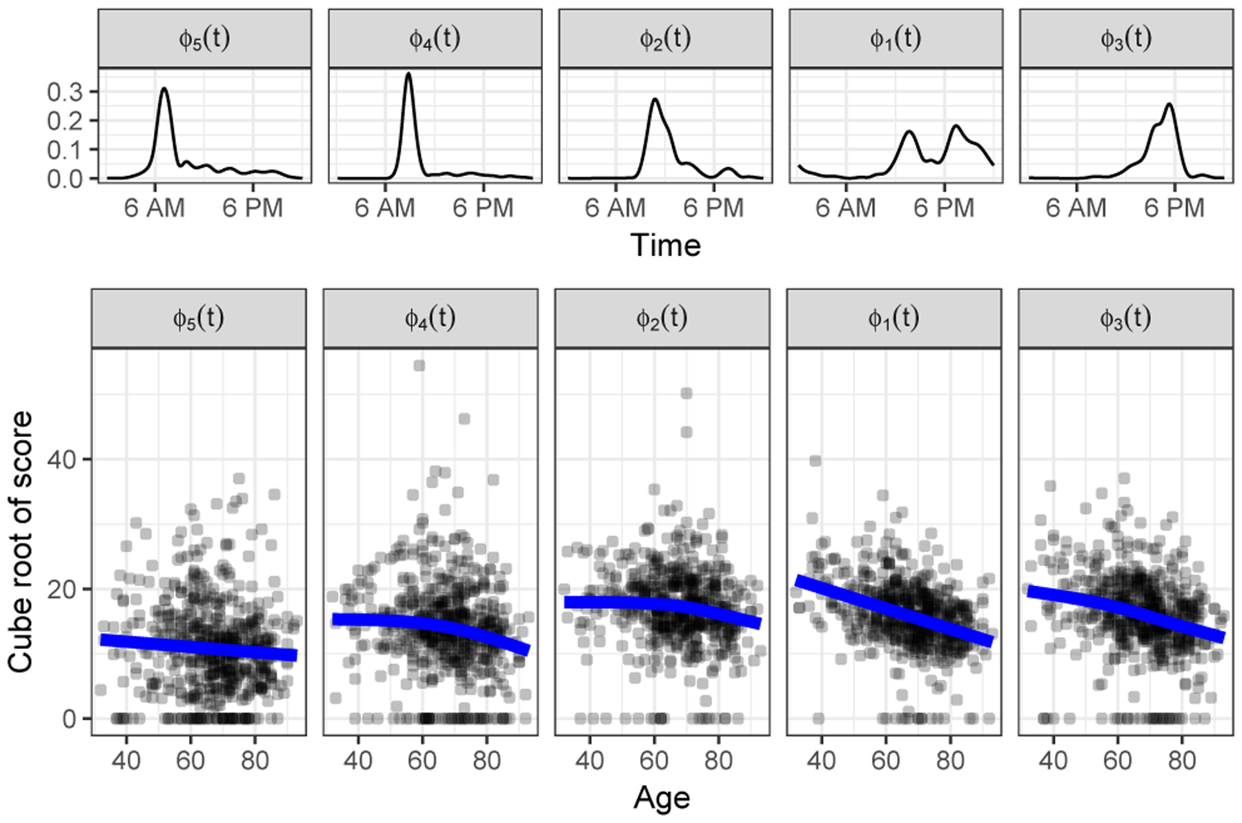
The cube root of NARFD scores for 592 subjects for each of 5 functional prototypes as a function of age (bottom). Functional prototypes (top) are ordered by the location of their peak, from early morning to evening. The lines show predictions from a generalized additive multivariate model fit to the cube root of the scores. A color version of this figure can be found in the electronic version of this article.

Lastly, we compare NARFD and GFPCA in terms of their ability to parsimoniously reconstruct observed curves. We fit each method to the data using from 1 to 12 functional prototypes/FPCs, using 50 subjects to estimate FPCs and then estimating scores for the remaining subjects. Figure 7 shows the negative Poisson log-likelihood for data from the held-out subjects for NARFD and GFPCA as a function of the number of functional prototypes/FPCs used in the decomposition. Unsurprisingly, NARFD requires more components to reconstruct the data than GFPCA, meaning that there is a tradeoff between interpretability and parsimony in the comparison of these methods for this data.

Figure 7.

Negative Poisson log-likelihood for held-out curves from BLSA data for NARFD and GFPCA, decomposed using 1 through 12 functional prototypes/FPCs estimated using 50 curves from the BLSA data. A color version of this figure can be found in the electronic version of this article.

Additional results in Section 3 of the supporting information illustrate the impact of changing the number of prototypes in the NARFD analysis, the results of a direct application of NMF (without smoothing) to these data, and repeated analysis under multiple random starting points. As expected, the NARFD prototypes differ somewhat as K increases; we also see that direct application of NMF produces difficult-to-interpret and very non-smooth results for these data, and that the NARFD prototypes across random starting points are broadly similar.

6. Discussion

We have introduced NARFD, a novel decomposition of non-negative functional count data which enables the study of patterns of variation across subjects in a highly interpretable manner. Applying these methods to our motivating dataset, we have extracted functional components which show clear peaks of activity at various times during the day. The accompanying scores can be used to classify subjects, and can be used as outcome variables to investigate the relationship between covariates and activity at different times of the day. We have also presented a novel algorithm for fitting GFPCA models for count data with a logarithmic link using alternating minimization.

A significant drawback of NARFD is that a unique solution is not guaranteed to exist. This limitation is inherent in methods based on non-negative matrix factorization, and is well-known in that context. Like others, we mitigate the impact of this issue by using a penalty to constrain the solution. In our application, estimated functional prototypes are consistent across random starting values and are recognizable as individual parts that combine to produce subject-level trajectories of physical activity. These results, together with our simulations, suggest that NARFD is reasonably well-posed in practice and can produce results that are more interpretable than those from GFPCA. In many data settings, including the use of accelerometers to measure physical activity, we expect that easily interpretable methods like NARFD will be favored by analysts and researchers, even when those methods have recognized limitations.

NARFD and GFPCA are methods for exponential family functional data (or “generalized functional data”), which is a relatively new topic in the functional data literature. Here, methods are concerned with settings where the functional data themselves take on non-Gaussian values across the observation domain, typified by 24-hour physical activity recordings of activity counts. Contributions in this area include efforts toward dimension reduction (Hall et al., 2008; van der Linde, 2009; Serban et al., 2013; Gertheiss et al., 2017), function-on-scalar regression (Goldsmith et al., 2015), and registration (Wrobel et al., 2018). For clarity, we draw a distinction between this literature and the literature for generalized functional linear regression models, which, in the context of the scalar-on-function regression models considered in Müller and Stadtmüller (2005), Du and Wang (2014), and many others, consider a non-Gaussian scalar outcome that depends on a functional predictor.

In general, it is difficult to determine the “optimal” number of prototypes to retain in an NMF-based analysis; see Wang and Zhang (2013) for a discussion. For NARFD, we recommend the use of a scree-like plot similar to Figure 3 to select the number of prototypes; alternatively, one might use cross-validation, although this may be time-consuming. A similar challenge (and similar solutions) arises for FPCA and GFPCA. Indeed, Wang et al. (2016) note with respect to FPCA that an “open question is the optimal choice of the number of components”. One possible direction for progress on this could follow Agniel et al. (2018), in which the authors develop a hypothesis test for variance components related to FPC score distributions, although substantial work remains even in the context of traditional FCPA.

Further extensions and refinements of NARFD could focus on the specification of separate smoothness penalties for each functional prototype/FPC. This would require the development of a new procedure for smoothness parameter selection, as our cross-validation procedure would become computationally infeasible with more than a few smoothness parameters. Our work has focused on curves that are completely observed over their domain, but in practice missing data is common especially in the context of wearable device data. Exploring NARFD as a possible approach for extrapolating observed data into periods of missingness or non-wear would be a useful practical contribution. Finally, with suitable modifications our method could be applied to data that has the normal, gamma or negative binomial distribution; these modifications may be useful in other scientific contexts.

A more challenging direction for future work would focus on multilevel non-negative functional data. In the BLSA, accelerometer data were collected across several days for each participant. As a preprocessing step, we aggregate counts across days to obtain a single curve for each subject that reflects a general activity pattern. Alternatively, one might wish to decompose curves for each subject and each day separately using a framework analogous to multilevel FPCA (Di et al., 2009; Goldsmith et al., 2015). This approach produces subject-level means and subject/day-level deviations, and can be appealing as a way to identify directions of variation that distinguish subjects and that distinguish days within a subject. Whether an analogous approach is possible using non-negative prototypes and scores is unclear, however, because subject/day-level deviations can be either positive or negative: a subject might be more active than his or her average on some days and less active on others. Despite this difficulty, extensions of NARFD to a multilevel setting would address issues that exist in real data.

Our focus is on the establishment of a framework for decomposing non-negative functional observations and the development of a robust estimation approach. Although inference for this method is not a primary interest, we comment briefly on a body of work for confidence intervals in the context of FPCA that may be useful for this problem. Briefly, for a given FPCA expansion (i.e. mean function, FPCs, and eigenvalues) obtain subject-specific scores using a mixed model. Inferential tools from this framework can then be used to obtain confidence intervals for subject-level fitted values (Yao et al., 2005). This assumes that the FPC expansion is “known”; Goldsmith et al. (2013) proposed a method that incorporates uncertainty in the FPCs using an approach built around (i) resampling to assess uncertainty in the decomposition and (ii) mixed-model inference for uncertainty given a specific decomposition. In principle, the same basic ideas could work for NARFD, although it is unclear whether resampling will suffice to assess uncertainty in the prototypes themselves and whether inferential tools from non-negative estimation are sufficient to obtain variance estimates for a given collection of prototypes. Moreover, there is a general need for contributions related to inference for NMF.

Temporal misalignment is a significant issue in FDA applications, and it is reasonable to anticipate variation in the timing and intensity of activity (referred to as “phase” and “amplitude” variation, respectively) in the BLSA accelerometer data. Registration can be particularly important in assessing population-level effects, which can be attenuated depending on the degree of misalignment across subjects. We argue that our focus on understanding and interpreting the directions of variation that underlie subject-level curves is useful even without registration as a preprocessing step or formal component of the analysis. It is likely that some subjects load more heavily on the “early morning” prototype and less heavily on “late night” prototype, and other subjects have the opposite activity pattern. Our method identifies these directions of variation (which do exist in the population), and allows identification of such subjects via scores. Registration, by contrast, would include this temporal variation in the warping functions; the result would be an ostensibly more parsimonious basis for amplitude variation at the cost of additional complexity in the warping functions that align temporal domains across subjects.

There are various techniques for dimension reduction that one might use in addition to traditional PCA-based methods. Many of these have not been readily adopted in functional data analysis, although they often have specific benefits in comparison to PCA and to each other. Our focus on adapting NMF to functional data stems from the popularity of this approach in general, with additional benefits in the context of our motivating data arising from the fact that the decomposition is carried out on the scale of the data and that the decomposition is strictly non-negative. That said, we see real promise in evaluating the usefulness of methods based on techniques other than PCA in the context of functional data.

As an example of an alternative approach to decomposition, a method suggested by a reviewer starts by applying a variance-stabilizing transformation (e.g., a square root transformation) to non-negative observations, and then applies standard FPCA techniques. When used for the BLSA data, this method yields reconstructions that are equivalently parsimonious to those of NARFD. However, like GFPCA, this method reconstructs observations on a latent scale, and the contributions of different FPCs to a reconstruction may cancel each other out; this method therefore lacks some of the interpretability advantages of NARFD. Other alternatives one might consider include adaptations of partial least squares or principal component pursuit methods to exponential family functional data.

References

- Agniel D, Xie W, Essex M, Cai T, et al. (2018). Functional principal variance component testing for a genetic association study of HIV progression. The Annals of Applied Statistics 12, 1871–1893. [DOI] [PMC free article] [PubMed] [Google Scholar]
- Bai J, He B, Shou H, Zipunnikov V, Glass TA, and Crainiceanu CM (2014). Normalization and extraction of interpretable metrics from raw accelerometry data. Biostatistics 15, 102–116. [DOI] [PMC free article] [PubMed] [Google Scholar]
- Bertsekas DP (2012). Incremental gradient, subgradient, and proximal methods for convex optimization: A survey In Sra S, Nowozin S, and Wright SJ, editors, Optimization for Machine Learning, chapter 4, pages 85–120. The MIT Press, Cambridge, Massachusetts. [Google Scholar]
- Box GEP and Cox DR (1964). An analysis of transformations (with discussion). Journal of the Royal Statistical Society B 26, 211–252. [Google Scholar]
- Brage S, Brage N, Ekelund U, Luan J, Franks PW, Froberg K, and Wareham NJ (2006). Effect of combined movement and heart rate monitor placement on physical activity estimates during treadmill locomotion and free-living. European Journal of Applied Physiology 96, 517–524. [DOI] [PubMed] [Google Scholar]
- Byrd RH, Lu P, Nocedal J, and Zhu C (1995). A limited memory algorithm for bound constrained optimization. SIAM Journal on Scientific Computing 16, 1190–1208. [Google Scholar]
- Collins M, S D, and E SR (2001). A generalization of principal component analysis to the exponential family In Proceedings of the 14th International Conference on Neural Information Processing Systems, pages 617–624. MIT Press. [Google Scholar]
- Di C-Z, Crainiceanu CM, Caffo BS, and Punjabi NM (2009). Multilevel functional principal component analysis. Annals of Applied Statistics 4, 458–488. [DOI] [PMC free article] [PubMed] [Google Scholar]
- Donoho DL and Stodden VC (2003). When does non-negative matrix factorization give a correct decomposition into parts? Advances in Neural Information Processing Systems 16, 1141–1148. [Google Scholar]
- Du P and Wang X (2014). Penalized likelihood functional regression. Statistica Sinica pages 1017–1041. [Google Scholar]
- Gertheiss J, Goldsmith J, and Staicu A-M (2017). A note on modeling sparse exponential-family functional response curves. Computational Statistics and Data Analysis 105, 46–52. [DOI] [PMC free article] [PubMed] [Google Scholar]
- Gillis N (2012). Sparse and unique nonnegative matrix factorization through data preprocessing. Journal of Machine Learning Research 13, 3349–3386. [Google Scholar]
- Goldsmith J, Greven S, and Crainiceanu CM (2013). Corrected confidence bands for functional data using principal components. Biometrics 69, 41–51. [DOI] [PMC free article] [PubMed] [Google Scholar]
- Goldsmith J, Zipunnikov V, and Schrack J (2015). Generalized multilevel function-on-scalar regression and principal component analysis. Biometrics 71, 344–353. [DOI] [PMC free article] [PubMed] [Google Scholar]
- Hall P, Müller H-G, and Yao F (2008). Modelling sparse generalized longitudinal observations with latent gaussian processes. Journal of the Royal Statistical Society: Series B 70, 703–723. [Google Scholar]
- Huang K, Sidiropoulos ND, and Swami A (2013). Non-negative matrix factorization revisited: Uniqueness and algorithm for symmetric decomposition. IEEE Transactions on Signal Processing 62, 211–224. [Google Scholar]
- Lee DD and Seung HS (1999). Learning the parts of objects by non-negative matrix factorization. Nature 401, 788–791. [DOI] [PubMed] [Google Scholar]
- Li Y and Ruppert D (2008). On the asymptotics of penalized splines. Biometrika 95, 415–436. [Google Scholar]
- Lin X and Boutros P (2016). NNLM: Fast and Versatile Non-Negative Matrix Factorization.
- Müller H-G and Stadtmüller U (2005). Generalized functional linear models. Annals of Statistics 33, 774–805. [Google Scholar]
- Ruppert D (2002). Selecting the number of knots for penalized splines. Journal of Computational and Graphical Statistics 11, 735–757. [Google Scholar]
- Schrack JA, Zipunnikov V, Goldsmith J, Bai J, Simonshick EM, Crainiceanu CM, and Ferrucci L (2014). Assessing the “physical cliff”: Detailed quantification of aging and physical activity. Journal of Gerontology: Medical Sciences. [DOI] [PMC free article] [PubMed] [Google Scholar]
- Serban N, Staicu A-M, and Carrol RJ (2013). Multilevel cross-dependent binary longitudinal data. Biometrics 69, 903–913. [DOI] [PMC free article] [PubMed] [Google Scholar]
- Shashua A and Hazan T (2005). Non-negative tensor factorization with applications to statistics and computer vision In Proceedings of the 22nd International Conference on Machine Learning, ICML ‘05, pages 792–799, New York, NY, USA: ACM. [Google Scholar]
- Smaragdis P and Brown J (2003). Non-negative matrix factorization for polyphonic music transcription, volume 2003-January, pages 177–180. Institute of Electrical and Electronics Engineers Inc. [Google Scholar]
- Sotiras A, Resnick SM, and Davatzikos C (2015). Finding imaging patterns of structural covariance via non-negative matrix factorization. NeuroImage 108, 1–16. [DOI] [PMC free article] [PubMed] [Google Scholar]
- Theis FJ, Stadlthanner K, and Tanaka T (2005). First results on uniqueness of sparse non-negative matrix factorization. In 2005 13th European Signal Processing Conference, pages 1–4. [Google Scholar]
- Udell M, Horn C, Zadeh R, and Boyd S (2016). Generalized low rank models. Foundations and Trends® in Machine Learning 9, 1–118. [Google Scholar]
- van der Linde A (2009). A Bayesian latent variable approach to functional principal components analysis with binary and count. Advances in Statistical Analysis 93, 307–333. [Google Scholar]
- Venables WN and Ripley BD (2002). Modern Applied Statistics with S. New York: Springer. [Google Scholar]
- Wang J-L, Chiou J-M, and Müller H-G (2016). Functional data analysis. Annual Review of Statistics and Its Application 3, 257–295. [Google Scholar]
- Wang Y and Zhang Y (2013). Nonnegative matrix factorization: A comprehensive review. IEEE Transactions on Knowledge and Data Engineering 25, 1336–1353. [Google Scholar]
- Wood SN (2011). Fast stable restricted maximum likelihood and marginal likelihood estimation of semiparametric generalized linear models. Journal of the Royal Statistical Society: Series B 73, 3–36. [Google Scholar]
- Wrobel J, Zipunnikov V, Schrack J, and Goldsmith J (2018+). Registration for exponential family functional data. Biometrics. [DOI] [PMC free article] [PubMed] [Google Scholar]
- Yao F, Müller H, and Wang J (2005). Functional data analysis for sparse longitudinal data. Journal of the American Statistical Association 100, 577–590. [Google Scholar]
- Ypma J (2017). nloptr: R interface to NLopt.
Associated Data
This section collects any data citations, data availability statements, or supplementary materials included in this article.