A Parameter Estimation Method for Multiscale Models of Hepatitis C Virus Dynamics

Abstract

Mathematical models that are based on differential equations require detailed knowledge about the parameters that are included in the equations. Some of the parameters can be measured experimentally while others need to be estimated. When the models become more sophisticated, such as in the case of multiscale models of hepatitis C virus dynamics that deal with partial differential equations (PDEs), several strategies can be tried. It is possible to use parameter estimation on an analytical approximation of the solution to the multiscale model equations, namely the long-term approximation, but this limits the scope of the parameter estimation method used and a long-term approximation needs to be derived for each model. It is possible to transform the PDE multiscale model to a system of ODEs, but this has an effect on the model parameters themselves and the transformation can become problematic for some models. Finally, it is possible to use numerical solutions for the multiscale model and then use canned methods for the parameter estimation, but the latter is making the user dependent on a black box without having full control over the method. The strategy developed here is to start by working directly on the multiscale model equations for preparing them toward the parameter estimation method that is fully coded and controlled by the user. It can also be adapted to multiscale models of other viruses. The new method is described and illustrations are provided using a user-friendly simulator that incorporates the method.

1. Introduction

Multiscale models have been introduced in recent years (Guedj et al., 2013a; Rong et al., 2013; Rong and Perelson, 2013; Quintela et al., 2018) to improve the modeling of hepatitis C viral (HCV) dynamics. Chronic HCV infection affects approximately 70 million people worldwide. It is the primary cause of liver cirrhosis, liver cancer and liver transplant (World Health Organization, 2014). There is no vaccine for HCV and for more than a decade the standard-of-care consisted of pegylated interferon-alpha (IFN) and ribavirin. The recent advent of direct-acting antivirals (DAAs) provided interferon-free, all-oral treatment yielding cure rates exceeding 90% with pangenotypic activity, shorter durations of therapy (8–24 weeks). Compared to IFN-based therapy (24–48 weeks) it is considered one of the greatest achievements in medicine (AASLD/IDSA HCV Guidance Panel, 2015). However, despite these highly effective DAAs, many challenges remain, such as finding an optimal approach to current DAA failures and reducing HCV infection and DAAs cost, which is a significant barrier in treating the populations that are most affected by HCV.

Mathematical modeling of HCV provides important insights. It has improved our understanding of intracellular viral genome dynamics (Guedj et al., 2013a; Dahari et al., 2009b, 2007; Neumann et al., 2010). The standard model for HCV kinetics during treatment has profoundly contributed to our assessment of the effectiveness and to our understanding of the mechanism of action of interferon-alpha and ribavirin (reviewed in (Dahari et al., 2009c, 2011)). The models were able to retrospectively predict the duration of treatment needed for HCV eradication under IFN-based therapies (Snoeck et al., 2010; Dixit et al., 2004; Guedj and Perelson, 2011) and more recently under IFN-free all oral DAAs (Dahari et al., 2016; Canini et al., 2017a; Gambato et al., 2018). Notably, the models were able to prospectively (i.e, in real time) predict the duration of IFN-free therapy needed to achieve cure (Dahari et al., 2015; Etzion et al., 2018). In the age of DAAs, new models have been developed to meet the challenges of these new agents such as drug resistance (Rong et al., 2010). Notably, the first age-based multiscale mathematical model for HCV kinetics was developed (Guedj et al., 2013a,b; Rong et al., 2013) and provided a comprehensive understanding of the nature of viral kinetic patterns observed in patients treated with IFN, HCV protease inhibitors (telaprevir and danoprevir), or HCV NS5A inhibitor daclatasvir and their modes of action. Mathematical models are also valuable in understanding the in vivo dynamics of viruses that trigger both persistent infection (e.g. HIV-1 (Perelson, 2002; Ho et al., 1995; Perelson et al., 1996; Burg et al., 2009), hepatitis B virus (Ciupe et al., 2007; Dahari et al., 2009d; Nowak et al., 1996), hepatitis D virus (Koh et al., 2015; Guedj et al., 2014; Canini et al., 2017b), Theiler murine encephalomyelitis virus (Zhang et al., 2013), herpes simplex virus (Schiffer et al., 2009) and HCV (Dahari et al., 2009a, 2005; Neumann et al., 1998)) and acute infection (e.g., influenza A (Baccam et al., 2006; Pawelek et al., 2012; Beauchemin and Handel, 2011) and ebola (Madelain et al., 2015)).

Multiscale models for HCV kinetics are an extension to the classical biphasic model (Neumann et al., 1998). The biphasic model treated the infected cell as a “black box”, producing virions but without any consideration of the intercellular viral RNA replication and degradation within the infected cell (Dahari et al., 2007, 2009b; Guedj and Neumann, 2010). It is a set of three ordinary differential equations (ODEs) with three variables: uninfected target cells (T), productively infected cells (I), and free virus (V). The multiscale models consider the intercellular viral RNA in an additional equation for the variable (R), with the introduction of age-dependency in addition to time-dependency, making it a partial differential equation (PDE) model. They are considerably more difficult to solve and to perform parameter estimation on compared to the biphasic model. Unlike the construction of numerical schemes in other applications, for example in the nonlinear diffusion of digital images (Weickert et al., 1998; Barash et al., 2001; Barash, 2005) where accuracy can be limited, herein it is advisable to construct a stable and efficient scheme that belongs to the Runge-Kutta family with a higher accuracy than in nonlinear diffusion. Our numerical solution strategy was outlined in (Reinharz et al., 2017, 2018) and herein, we continue (Reinharz et al., 2018) by providing a parameter estimation method that follows this strategy.

Parameter estimation (or callibration) of multiscale HCV models with HCV kinetic data measured in treated patients are challenging. To overcome this, several strategies were employed. The first strategy, employed in (Rong et al., 2013), utilizes an analytical solution named long-term approximation for solving the model equations along with calling the Levenberg-Marquardt (Levenberg, 1944; Marquardt, 1963) as a canned method for performing the fitting. The second strategy, employed in (Kitagawa et al., 2018), transforms the multiscale model to a system of ODEs and as such, simple parameter estimation methods can be used in the same manner as for the biphasic model. The third strategy, employed in (Quintela et al., 2018), is based on the method of lines and utilizes canned methods for both the numerical solution of the resulting equations (Matlab’s ode45) and for performing the fitting (Matlab’s fmincon). In contrast from all these approaches, our strategy does not rely on any canned method but fully implements our own Levenberg-Marquardt routine, thus making it suitable to other multiscale model equations by modifications inside the routine and an early preparation of the multiscale equations by taking their deriatives with respect to the parameters we would like to estimate. In the continuation, we will discuss why this strategy is advantageous.

The aim of this paper is to improve on parameter estimation methods for multiscale models that up until now, used canned routines (routines called from by a command within a program that is written in a higher level langauage such as Matlab and Mathematica, or Python) in a limited way that does not exert full control by the user. This makes the framework for parameter estimation as explained herein and distributed free of charge along with a user-friendly GUI a flexible and robust entity alongside the previous methods. Up until now the previous methods were sufficient for specific cases worked out for a particular multiscale model or a numerical solution with small timesteps, but they may likely suffer from problematic issues when coping with more extended simulations and diverse cases, without a simulator to experiment with. Starting from a description of the parameters and simulated data from patients, we first re-visit the numerical solutions and corresponding notations that were worked out in (Reinharz et al., 2018), extending the Jacobian matrix and providing a detailed description of Levenberg-Marquardt for our application. We then describe in a step-by-step procedure how to prepare the multiscale model equations for our parameter estimation method by taking their derivatives with respect to the various parameters. Along with showing the results using our built-in simulator with a user friendly GUI, we discuss the results reached and the advantages of our strategy in performing parameter estimation directly from the equations of the multiscale models.

2. Multiscale Models for HCV Dynamics

A multiscale model for HCV infection and treatment dynamics (Figure 1) was introduced in (Rong et al., 2013; Guedj et al., 2013a; Rong and Perelson, 2013). Intracellular HCV RNA plays a biologically significant role during the HCV replication and mutliscale models are considering it by additional equations for the RNA that are age-dependent, with the most complete model to date that was recently put forth in (Quintela et al., 2018). Figure 1 contains all the parameters that were used in the multiscale model described in (Rong et al., 2013), which forms an example of our parameter estimation calibration method for PDE models developed herein that can easily be extended to include additional parameters. All the parameters of the models can be seen in Table 1.

Fig. 1.

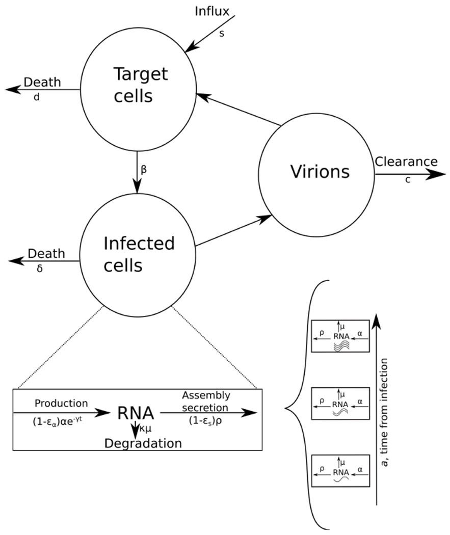
A schematic diagram of the HCV multiscale model and the inclusion of the virus RNA replication in the model.

Table 1.

The 12 parameters of the model.

s (cells mL−1)	Influx rate of new hepatocytes
d (d−1)	Target cell loss/death rate constant
β (mL d−1 virion−1)	Infection rate constant
δ (d−1)	HCV-infected cell loss/death rate constant
ρ (d−1)	Virion assembly / secretion rate constant
c (d−1)	Virion clearance rate constant
α (vRNAd−1)	vRNA synthesis rate
μ (d−1)	vRNA degradation
κ	Enhancement of intracellular viral RNA degradation
γ (d−1)	Loss rate of vRNA replication complexes
εs	Treatment vs secretion / assembly effectiveness
εα	Treatment vs production effectiveness

2.1. Model Equations

The multiscale model (Rong et al., 2013; Guedj et al., 2013a; Rong and Perelson, 2013) can be formulated as follows:

$$\frac{\text{d}T\left(t\right)}{\text{d}t}=s-dT\left(t\right)-\beta V\left(t\right)T\left(t\right)$$ (1a)

$$\frac{\partial I\left(a,t\right)}{\partial t}+\frac{\partial I\left(a,t\right)}{\partial a}=-\delta I\left(a,t\right)$$ (1b)

$$\frac{\text{d}V\left(t\right)}{\text{d}t}=\left(1-{\epsilon }_s\right){\int }_0^{\infty }\rho R\left(a,t\right)I\left(a,t\right)\text{d}a-cV\left(t\right)$$ (1c)

$$\frac{\partial R\left(a,t\right)}{\partial t}+\frac{\partial R\left(a,t\right)}{\partial a}=\left(1-{\epsilon }_{\alpha }\right)\alpha {\text{e}}^{-\gamma t}-\left(\left(1-{\epsilon }_s\right)\rho +\kappa \mu \right)R\left(a,t\right).$$ (1d)

The four variables this model keeps track of are the target cells T, in Eq. (1a), the infected cells I in Eq. (1b), the free virus V in Eq. (1c) and the intracellular viral RNA R in an infected cell, in Eq. (1d).

The target cells T are produced at constant rate s, and decrease by the number of cells infected by virus in blood V at constant rate β and their death at per capita rate d. The infected cells I die at constant per capita rate δ. The quantity of intracellular viral RNA R depends on its production α and its degradation μ and expulsion from the cell ρ. The quantity of free virus V depends on the number of assembled and released virions and their clearance rate c. The parameter γ represents the decay of replication template under therapy. The decrease in viral RNA synthesis is represented by ε_α, the reduction in secretion by ε_s and the increase in viral degradation by κ ≥ 1.

An important consideration in this model is that the treatment starts after the infection has reached its steady state. We denote by t the time since the beginning of treatment, which is set to zero at the beginning of our simulation. Another different time is a, which represents the age of the cell. The steady states of the different variables are $\stackrel{\_}{R}(a)$, $\stackrel{\_}{I}(a)$, $\stackrel{\_}{V}$ and $\stackrel{\_}{T}$. The term N represents the total number of virions produced by infected cells.

At steady state, the initial and boundary conditions are: $T(0)=\stackrel{\_}{T}$, $V(0)=\stackrel{\_}{V}$, I(0, t) = βV(t)T(t), $I(a,0)=\stackrel{\_}{I}(a)$, R(0, t) = 1, and $R(a,0)=\stackrel{\_}{R}(a)$.

These values have been previously derived in (Rong et al., 2013) and can be expressed as follows:

$$\stackrel{\_}{T}=c/\beta N$$ (2a)

$$\stackrel{\_}{V}=\left(\beta Ns-dc\right)/\left(\beta c\right)$$ (2b)

$$\stackrel{\_}{I}\left(a\right)=\beta \stackrel{\_}{V}\stackrel{\_}{T}{\text{e}}^{-\delta a}$$ (2c)

$$\stackrel{\_}{R}\left(a\right)=\frac{\alpha }{\rho +\mu }+\left(1-\frac{\alpha }{\rho +\mu }\right){\text{e}}^{-\left(\rho +\mu \right)\left(a\right)}$$ (2d)

$$N=\frac{\rho \left(\alpha +\delta \right)}{\delta \left(\rho +\mu +\delta \right)}$$ (2e)

Additionally, the equations for I(a, t) and R(a, t) can be solved by the method of characteristics to yield:

$$I\left(a,t\right)=\{\begin{array}{ll}\beta V\left(t-a\right)T\left(t-a\right){\text{e}}^{-\delta a}& a<t\\ \stackrel{\_}{I}\left(a-t\right){\text{e}}^{-\delta t}=\beta \overline{V}\overline{T}{\text{e}}^{-\delta a}=\left(\beta Ns-dc\right)/\left(\beta N\right){\text{e}}^{-\delta a}& a>t\end{array}$$ (3)

and

$$R\left(a,t\right)=\{\begin{array}{ll}\frac{\left(1-{\epsilon }_{\alpha }\right)\alpha {\text{e}}^{-\gamma t}}{\left(1-{\epsilon }_s\right)\rho +\kappa \mu -\gamma }+\left(1-\frac{\left(1-{\epsilon }_{\alpha }\right)\alpha {\text{e}}^{-\gamma \left(t-a\right)}}{\left(1-{\epsilon }_s\right)\rho +\kappa \mu -\gamma }\right){\text{e}}^{-\left(\left(1-{\epsilon }_s\right)\rho +\kappa \mu \right)a}& a<t\\ \frac{\left(1-{\epsilon }_{\alpha }\right)\alpha {\text{e}}^{-\gamma t}}{\left(1-{\epsilon }_s\right)\rho +\kappa \mu -\gamma }+\left(\frac{\alpha }{\rho +\mu }+\left(1-\frac{\alpha }{\rho +\mu }\right){\text{e}}^{-\left(\rho +\mu \right)\left(a-t\right)}-\frac{\left(1-{\epsilon }_{\alpha }\right)\alpha }{\left(1-{\epsilon }_s\right)\rho +\kappa \mu -\gamma }\right){\text{e}}^{-\left(\left(1-{\epsilon }_s\right)\rho +\kappa \mu \right)t}& a>t\end{array}$$ (4)

The main goal of these equations is to allow us to predict the number of virions present after a certain time t of treatment, when all the parameters are known. The challenge we would like to tackle is whether given the change in the virion load of a patient, we can estimate the treatment parameters (ε_s, ε_α, γ, and κ) and thereby understand how the treatment works.

2.2. Model Parameters and Data from Patients

The multiscale model was calibrated with data from treated patients by (Rong et al., 2013). The data points to fit the model and on which the error is computed are only V. While the raw data is not available, we used the freely accessible tool by (Rohatgi, 2018) to retrieve it from a figure directly. The result for one patient is displayed in Fig. 2. We set $\stackrel{\_}{V}$ as the pre-treatment viral load observed in the patient.

Fig. 2.

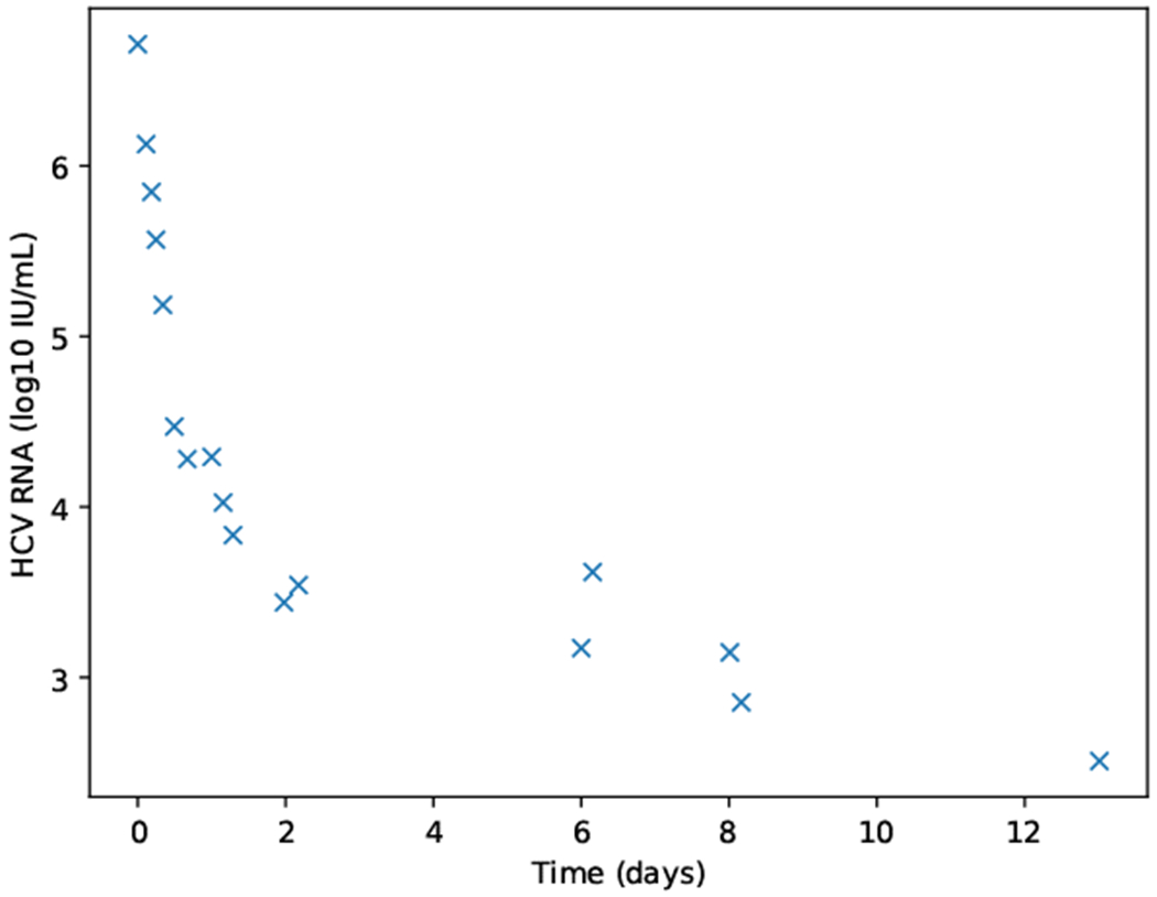
Datapoints retrieved with the WebPlotDigitizer tool by (Rohatgi, 2018). Data was extracted from (Rong et al., 2013) for a patient that was treated with the HCV protease inhibitor danoprevir.

In our method, we mostly use the default parameters from (Rong et al., 2013) that are shown in Table 2. To maintain the equality of Eq. (2b) we must change one parameter. Inspired by the method of (Rong et al., 2013), we chose to fix all parameters except s. For a patient the value of s is determined by its $\stackrel{\_}{V}$ and by Eq. (2b), such that $s=(\stackrel{\_}{V}\beta c+dc)/(\beta N)$, where N is taken from Eq. (2e).

Table 2.

Default parameters that are used herein. Parameter s comes from Eq. (2b), taking $\stackrel{\_}{V}$ as the max Virions value.

α	40 d−1	β	5 × 10−8 mL d−1
c	22.3 d−1	δ	0.14 d−1
μ	1 d−1	d	0.01 d−1
ρ	8.18 d−1	s	$(\stackrel{\_}{V}\beta c+cc)/(\beta N)\text{cells}/\text{mL}$

To verify that we can fix s given $\stackrel{\_}{V}$, we show in Figure 3 how a system starting with 1 × 10⁸ target cells and 100 virions reaches steady state depending on the value of s. In blue the parameter s is set to 130 000 as in (Rong et al., 2013) and in orange to 475 573. This latter value was computed with the strategy described in the previous paragraph. As observed, both curves have the same shape, and the steady state reached by setting s to 475 573 is consistent with the extracted data.

Fig. 3.

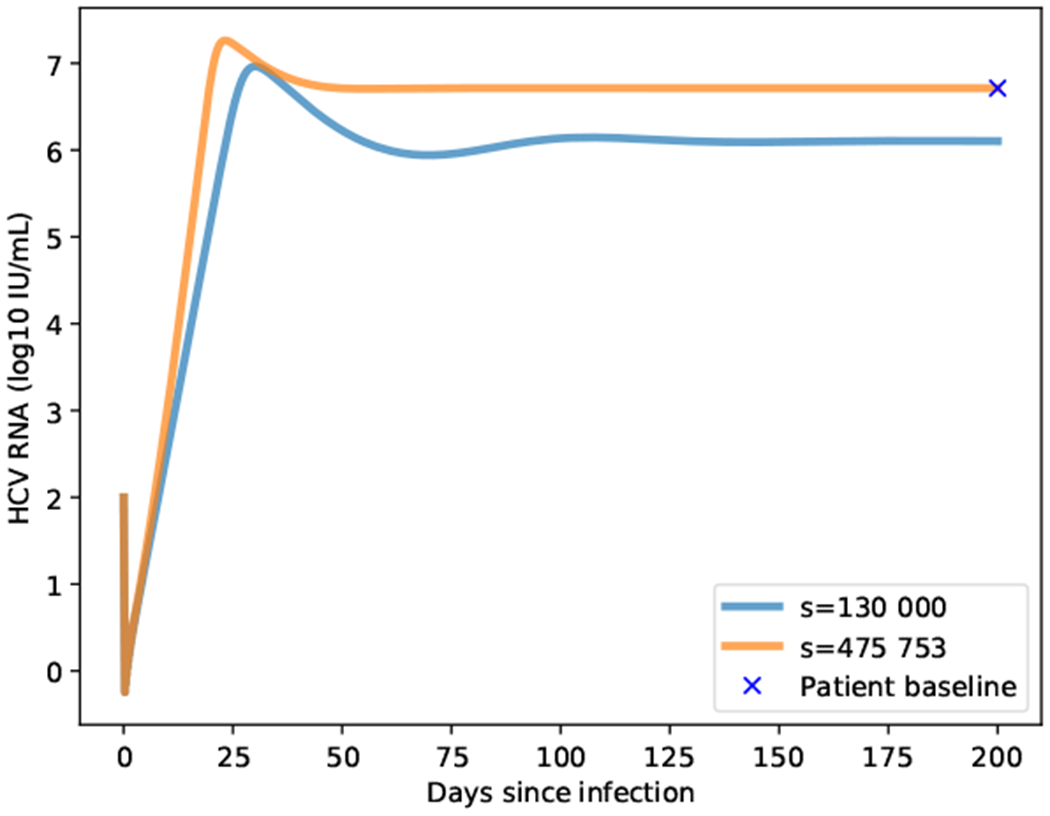
Virions change reaching the steady states with two different values of s. In blue with s = 130 000 as reported in (Rong et al., 2013). In orange with s = 475573 as computed with Eq. (2b) given $\stackrel{\_}{V}$ the baseline observed in the patient, shown as a blue x.

Because T is also unknown and we assume that we start at a steady state, we compute it using the default parameters and Eq. (2a).

2.3. Analytical approximations and Numerical Solutions of the Multiscale Model Equations

As discussed in (Reinharz et al., 2018), the analytical approximations for the multiscale model have some limitations. The long-term approximation that is used in practice is an underestimate of the amount of HCV RNA in the model since some infection events are being ignored. Moreover, for each multiscale model the long-term approximation needs to be derived analytically. Thus, numerical solutions provide an attractive alternative and could be easier to adjust when introducing changes to the model. A more general and comprehensive approach to parameter fitting without relying on analytical approximations would be useful. And although it was recently shown that it is possible to transform the PDE multiscale model to a system of ODEs (Kitagawa et al., 2018), this transformation problematically introduces some of the boundary conditions, e.g. ζ, as new parameters inside the model equations. A numerical approach to parameter fitting of multiscale models was recently put forth and described in (Quintela et al., 2018), by the use of the method of lines and canned methods that are available in Matlab. Our new numerical approach that originated in (Reinharz et al., 2018) and described herein does not rely on canned methods, with considerable benefits that will be discussed in the continuation.

For the numerical solution of the multiscale model equations, we showed in (Reinharz et al., 2018) that the full implementation of the Rosenbrock method is preferable over the use of a canned solver in terms of efficiency and stability. Therefore the Rosenbrock method has been implemented for the purpose of our parameter fitting method as well. In order to apply the Rosenbrock method, it is simplest to represent the system to be solved as a vector f of two functions:

$$y\prime =f\left(t,y\right)=\left[\frac{\text{d}T}{\text{d}t},\frac{\text{d}V}{\text{d}t}\right]=\left[s-dT-\beta VT,\left(1-{\epsilon }_s\right){\int }_0^{\infty }\rho R\left(a,t\right)I\left(a,t\right)\text{d}a-cV\right],$$ (5)

where y is a vector with the values of [T, V]. This representation has originated in (Reinharz et al., 2018) for convenience with formulating the numerical schemes described in that reference. This function depends on 3 variables, t, V and T. While V and T are the values at the time point we are evaluating, inside the equation of I the function V(t − a) and T(t − a) do depend on t directly. In our implementation, when computing the integral, we need to divide into two cases. If a > t, we analytically determine the values of R(a, t) and I(a, t) for small time steps a. When a < t, the system was previously solved at times τ₀, …, τ_n. Therefore we evaluate the integrals at times a₀ = t − τ₀, …, a_n = t − τ_n, ensuring that the required values of V(t − a) and T(t − a) are already known, following the scheme presented in (Reinharz et al., 2018).

The Rosenbrock method additionally requires the Jacobian matrix, denoted by f′. While in (Reinharz et al., 2018) the integral terms were ignored in the Jacobian, we now explicitly include them since in some cases their values cannot be ignored for the purpose of parameter estimation, as will be discussed in Sec. 3.2.

The fully derived Jacobian matrix is:

$$f\prime =\left(\begin{array}{cc}-d-\beta V& -\beta T\\ \left(1-{\epsilon }_s\right){\int }_0^t\rho R\left(a,t\right)\times \frac{\partial I\left(a,t\right)}{\partial T}\text{d}a& \left(1-{\epsilon }_s\right){\int }_0^t\rho R\left(a,t\right)\times \frac{\partial I\left(a,t\right)}{\partial V}\text{d}a-c\end{array}\right)$$ (6)

where we have

$$\frac{\partial I\left(a,t\right)}{\partial T}=\{\begin{array}{ll}\beta \left(\frac{\partial V\left(t-a\right)}{\partial T}T\left(t-a\right)+V\left(t-a\right)\frac{\partial T\left(t-a\right)}{\partial T}\right){\text{e}}^{-\delta a}& a<t\\ 0& a>t\end{array}$$ (7)

and

$$\frac{\partial I\left(a,t\right)}{\partial V}=\{\begin{array}{ll}\beta \left(\frac{\partial V\left(t-a\right)}{\partial V}T\left(t-a\right)+V\left(t-a\right)\frac{\partial T\left(t-a\right)}{\partial V}\right){\text{e}}^{-\delta a}& a<t\\ 0& a>t\end{array}.$$ (8)

If we let T_a := T(t−a), then we may regard T_a as a function of t via T by writing T_a = T_a(T(t)). Then $\frac{\text{d}{T}_a}{\text{d}t}=\frac{\text{d}{T}_a}{\text{d}T}\frac{\text{d}T}{\text{d}t}=\frac{\partial T_a}{\partial T}\frac{\text{d}T}{\text{d}t}$, so that $\frac{\partial T_a}{\partial T}=\frac{\text{d}{T}_a}{\text{d}t}/\frac{\text{d}T}{\text{d}t}$, and $\frac{\partial T(t-a)}{\partial T}=\frac{\text{d}T(t-a)}{\text{d}t}/\frac{\text{d}T}{\text{d}t}$. Analogously, $\frac{\partial V(t-a)}{\partial V}=\frac{\text{d}V(t-a)}{\text{d}t}/\frac{\text{d}V}{\text{d}t}$, $\frac{\partial V(t-a)}{\partial T}=\frac{\text{d}V(t-a)}{\text{d}t}/\frac{\text{d}V}{\text{d}t}$, and $\frac{\partial T(t-a)}{\partial V}=\frac{\text{d}T(t-a)}{\text{d}t}/\frac{\text{d}V}{\text{d}t}$. All these values are directly calculated with eq (5).

Because we are starting from the steady state then some of the derivatives, for example $\frac{\text{d}T}{\text{d}t}$, are initially zero. We observe that this singularity is only present in the first time step. In previous work (Reinharz et al., 2018) we noticed that omitting the integral term from the Jacobian still allows us to reach an approximation of the PDE system that is very close to the long-term approximation. Therefore only for the first time step, when the singularity is present, we set the integral term to zero.

Additionally, we need to add the term $\frac{\partial f}{\partial t}$, which is expressed as follows. We note that $\frac{\partial I}{\partial t}=0$ when a > t since from Eq. (3) the value of I does not in that case depend on t.

$$\frac{\partial f}{\partial t}=\left[0,\left(1-{\epsilon }_s\right){\int }_0^{\infty }\rho \left(\frac{\partial R\left(a,t\right)}{\partial t}I\left(a,t\right)+R\left(a,t\right)\frac{\partial I\left(a,t\right)}{\partial t}\right)\text{d}a\right],$$ (9)

where:

$$\frac{\partial I\left(a,t\right)}{\partial t}=\{\begin{array}{ll}\beta \left(\frac{\partial V\left(a,t\right)}{\partial t}T\left(t-a\right)+V\left(t-a\right)\frac{\partial T\left(t-a\right)}{\partial t}\right){\text{e}}^{-\delta a}& a<t\\ 0& a>t\end{array}$$ (10)

By definition of the ordinary and partial derivatives in this case, we find that $\frac{\partial T(t-a)}{\partial t}=\frac{\text{d}T(t-a)}{\text{d}t}$ and $\frac{\partial V(t-a)}{\partial t}=\frac{\text{d}T(t-a)}{\text{d}t}$, which allows us to evaluate $\frac{\partial T(t-a)}{\partial t}$ and $\frac{\partial V(t-a)}{\partial t}$ directly from Eq. (1a) and Eq. (1c), respectively. Additionally,

$$\begin{gathered} \frac{\partial R\left(a,t\right)}{\partial t}=\{\begin{array}{ll}-\gamma \frac{\left(1-{\epsilon }_{\alpha }\right)\alpha {\text{e}}^{-\gamma t}}{\left(1-{\epsilon }_s\right)\rho +\kappa \mu -\gamma }+\gamma \frac{\left(1-{\epsilon }_{\alpha }\right)\alpha {\text{e}}^{-\gamma \left(t-a\right)}}{\left(1-{\epsilon }_s\right)\rho +\kappa \mu -\gamma }{\text{e}}^{-\left(\left(1-{\epsilon }_s\right)\rho +\kappa \mu \right)a}& a<t\\ -\gamma \frac{\left(1-{\epsilon }_s\right)\alpha {\text{e}}^{-\gamma t}}{\left(1-{\epsilon }_s\right)\rho +\kappa \mu -\gamma } \\ +\left(\left(\rho +\mu \right)\left(1-\frac{\alpha }{\rho +\mu }\right){\text{e}}^{-\left(\rho +\mu \right)\left(a-t\right)}\right){\text{e}}^{-\left(\left(1-{\epsilon }_s\right)\rho +\kappa \mu \right)t} \\ +\left(\frac{\alpha }{\rho +\mu }+\left(1-\frac{\alpha }{\rho +\mu }\right){\text{e}}^{-\left(\rho +\mu \right)\left(a-t\right)}-\frac{\left(1-{\epsilon }_{\alpha }\right)\alpha }{\left(1-{\epsilon }_s\right)\rho +\kappa \mu -\gamma }\right) \\ \times (({\epsilon }_s-1)\rho -\kappa \mu ){\text{e}}^{-\left(\left(1-{\epsilon }_s\right)\rho +\kappa \mu \right)t}& a>t\end{array} \end{gathered}$$ (11)

3. Issues of Parameter Estimation and Optimization Procedure

3.1. Preliminaries

The HCV multiscale model described in (Rong et al., 2013) has 12 parameters (Table 1) and the nonlinear differential equations that comprise it are stiff (Reinharz et al., 2018). In addition, the integral term in the equation complicates matters, as described in (Reinharz et al., 2018). Parameter fitting is known to be a difficult problem in general and for multiscale models, in particular, one needs to approach it carefully with the use of robust techniques for the optimization.

The widely used Levenberg–Marquardt method (Levenberg, 1944; Marquardt, 1963) allows to fit an ensemble of parameters and has been shown to produce convincing results in simpler models than multiscale models. It does not guarantee that one will find a global optimum but given a set of reasonable starting points, in practice a sufficiently good local minimum can be found. Previous results as in (Rong et al., 2013) have shown the suitability of the Levenberg–Marquardt method for the optimization of multiscale models. Additionally, the implementation of the Rosenbrock method (Rosenbrock, 1963) by (Reinharz et al., 2018) can be extended to obtain the terms required by the Levenberg–Marquardt method, as explained in Sec. 3.2. We present in Fig. 4 a flow diagram of the procedure.

Fig. 4.

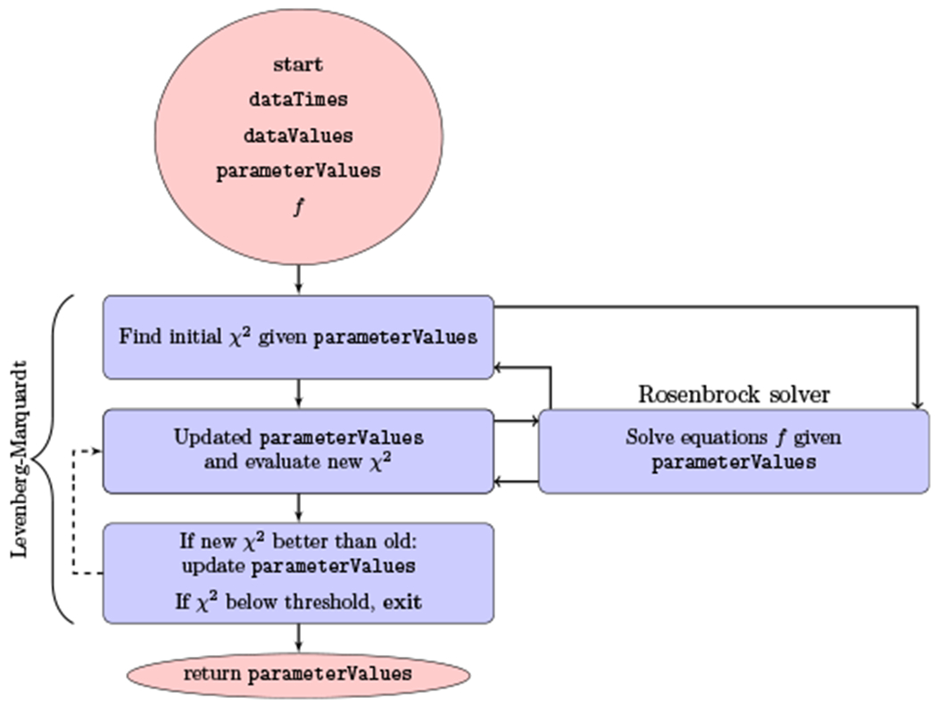
Flow diagram of the strategy with the implemented parameter estimator. The inputs are a list of data values dataValues taken at different times dataTimes. It also requires an initial guess for the ensemble of parameters parameterValues and the vector of functions f that are needed to perform the fitting. The χ² merit function refers to the error given parameterValues.

3.2. Optimization by Levenberg–Marquardt

The Levenberg–Marquardt method is implemented in our newly introduced parameter estimation method as a major component. It is an iterative numerical method that leverages the gradient vector and the Jacobian matrix to find a local minimum depending on the starting parameters.

The general method can be summarized as follows (Press et al., 1997). Given are a vector m of m data points with a measure of uncertainty of the i^th measurement σ_i (i ∈ [1, ⋯, m]) and a vector p of parameters. If a solution to Eq. (5) is y (the vector [T, V]), the model to be fitted is:

$$y=y\left(t|\mathbf{p}\right),$$ (12)

where t_i, i ∈ [1, ⋯, m] are the m times associated with m.

To evaluate the quality of p, a dimensionless number χ² is used as a merit function and is defined as:

$${\chi }^2=\sum _{i=1}^m{\left[\frac{y_i-y\left(t_i|\mathbf{\text{p}}\right)}{{\sigma }_i}\right]}^2,$$ (13)

where y_i is the observed value of the parameter y at time t_i.

At each iteration, a tentative new vector p+δp is computed and depending on χ² the value is accepted or rejected. The change in parameter l of p, denoted by δp_l, is computed by solving the system of linear equations:

$$\sum _{l=1}^m{\zeta }_{kl}{\delta }_{pl}={\xi }_l,$$ (14)

where ξ_l, defined as $-\frac{1}{2}\frac{\partial {\chi }^2}{\partial {\delta }_{p_l}}$, depends on the gradients of y as a function of the parameters and ζ_kl, defined as $\frac{1}{2}\frac{{\partial }^2{\chi }^2}{\partial {\delta }_{p_k}\partial {\delta }_{p_l}}$, depends on the partial derivatives of χ² as a function of the parameter p_l.

The following observations allow to determine the gradients of y as a function of any parameter. Solving Eq. (5) returns y, therefore we can take $\frac{\partial y}{\partial p_l}$ to be the solution of $\frac{\partial y\prime }{\partial p_l}=\frac{\partial f}{\partial p_l}(t,y^{p_l})$, which is:

$$\frac{\partial f}{\partial p_l}\left(t,y^{p_l}\right)=\left[\frac{\partial \frac{\text{d}T}{\text{d}t}}{\partial p_l},\frac{\partial \frac{\text{d}V}{\text{d}t}}{\partial p_l}\right]=\left[\frac{\partial }{\partial p_l}\left(s-dT-\beta VT\right),\frac{\partial }{\partial p_l}\left(\left(1-{\epsilon }_s\right){\int }_0^{\infty }\rho R\left(a,t\right)I\left(a,t\right)\text{d}a-cV\right)\right],$$ (15)

where y^p_l is the vector $[T,V\frac{\partial T}{\partial p_l},\frac{\partial V}{\partial p_l}]$. From Clairaut’s theorem on the equality of mixed partial derivatives, we have that $[\frac{\partial \frac{\text{d}T}{\text{d}t}}{\partial p_l},\frac{\partial \frac{\text{d}V}{\text{d}t}}{\partial p_l}]=[\frac{\text{d}\frac{\partial T}{\partial p_l}}{\text{d}t},\frac{\text{d}\frac{\partial V}{\partial p_l}}{\text{d}t}]$, which allows us to solve with respect to t to compute the values of the partial derivatives.

The partial derivative of the second term could cause a problem due to the integral term. In practice, the integration is performed over 0 to 100, the maximal age of a cell. Therefore, by the Leibniz integral rule, we can exchange the integral and the derivative to obtain:

$$\frac{\partial f}{\partial p_l}\left(t,y^{p_l}\right)=\left[\frac{\partial }{\partial p_l}\left(s-dT-\beta VT\right),{\int }_0^{\infty }\frac{\partial }{\partial p_l}\left(\left(1-{\epsilon }_s\right)\rho R\left(a,t\right)I\left(a,t\right)\text{d}a\right)-\frac{\partial }{\partial p_l}\left(cV\right)\right].$$ (16)

It should be noticed that in the multiscale model the integral term in the Jacobian matrix is negligible, being dominated by the value of β in I(a, t), which is of the order of 10⁻⁸. This is not true when generalized for the ensemble of parameters that need to be solved since the integral in Eq. (16) can become quite complex. As an example, the case where the parameter β needs to be fitted will necessarily have a term without it in the integral. This case is shown in the Appendix.

Due the large difference in the scale of the number of virions over a few days, fitting only for the value of V would not return accurate results since the fitting would mostly consider the first few data points. While for the value of log V we can solve Eq. (1c) and simply take the log, we must take an extra step when computing the derivatives in our scheme. This can be resolved with the observation that:

$$\frac{\partial \log \left(V\right)}{\partial p}=\frac{1}{V}\frac{\partial V}{\partial p}.$$ (17)

Because our method solves the equations for V and $\frac{\partial V}{\partial p}$ simultaneously, we apply before using the results the log to V and divide $\frac{\partial V}{\partial p}$ by V, therefore obtaining the correct values.

3.3. Parameter Estimation Performed Directly from the Equations

To fit any parameter, an ensemble of equations needs to be directly implemented by taking their derivatives. We provide the implementation for the following 10 parameters: s, d, β, ρ, ε_s, ε_α, κ, c, δ, and γ.

Two of the model parameters were not included, α and μ. This is due to the fact that in the model we always have (1 − ε_α)α and κμ. Therefore fitting one or the other parameter is sufficient because it is impossible to know which of the two parameters should actually change.

For each parameter, the equations are different, but the same procedure needs to be applied to derive all of them. For illustration, we provide the procedure for the parameters ρ, s, γ.

3.3.1. Parameter ρ

The main observation is that in order to fit the parameter ρ on the function V, we must be able to compute the partial derivative of V with respect to ρ, denoted by $\frac{\partial V}{\partial \rho }$. To do so, we can leverage our implementation of the Rosenbrock method for solving V. It follows from Eq. (5) that:

$$\frac{\partial f}{\partial \rho }\left(t,y^{\rho }\right)=\left[-d\frac{\partial T}{\partial \rho }-\beta \left(\frac{\partial V}{\partial \rho }T+V\frac{\partial T}{\partial \rho }\right),\left(1-{\epsilon }_s\right){\int }_0^{\infty }\left(R\left(a,t\right)I\left(a,t\right)+\rho \frac{\partial R\left(a,t\right)}{\partial \rho }I\left(a,t\right)+\rho R\left(a,t\right)\frac{\partial I}{\partial \rho }\left(a,t\right)\right)\text{d}a-c\frac{\partial V}{\partial \rho }\right],$$ (18)

where y^ρ is a vector with the values of $[T,V\frac{\partial T}{\partial \rho },\frac{\partial V}{\partial \rho }]$.

The initial and boundary conditions can be derived by taking the partial derivative on each term. Thus, we have $\frac{\partial T}{\partial \rho }(0)=\frac{\partial \stackrel{\_}{T}}{\partial \rho }$, $\frac{\partial V}{\partial \rho }(0)=\frac{\partial \stackrel{\_}{V}}{\partial \rho }$, $\frac{\partial I}{\partial \rho }(0,t)=\beta (\frac{\partial V}{\partial \rho }(t)T(t)+V(t)\frac{\partial T}{\partial \rho }(t))$, $\frac{\partial I}{\partial \rho }(a,0)=\frac{\partial \stackrel{\_}{I}}{\partial \rho }(a)$, $\frac{\partial R}{\partial \rho }(0,t)=0$, and $\frac{\partial R}{\partial \rho }(a,0)=\frac{\partial \stackrel{\_}{R}}{\partial \rho }(a)$.

Given that:

$$\frac{\partial N}{\partial \rho }=\frac{\left(\alpha +\delta \right)}{\delta \left(\rho +\mu +\delta \right)}-\frac{\delta \rho \left(\alpha +\delta \right)}{{\left(\delta \left(\rho +\mu +\delta \right)\right)}^2}$$ (19)

the other terms can be simplified as follows:

$$\begin{gathered} \frac{\partial \overline{T}}{\partial \rho }=-\frac{c\delta \left(\mu +\delta \right)}{\beta \left(\alpha +\delta \right){\rho }^2} \\ \frac{\partial \overline{V}}{\partial \rho }=\frac{s\left(\alpha +\delta \right)\left(\mu +\delta \right)}{c\delta {\left(\rho +\mu +\delta \right)}^2} \\ \frac{\partial \overline{I}}{\partial \rho }\left(a\right)=\beta \left(\frac{\partial \overline{V}}{\partial \rho }\overline{T}+\overline{V}\frac{\partial \overline{T}}{\partial \rho }\right){\text{e}}^{-\delta a} \\ \frac{\partial \overline{R}}{\partial \rho }\left(a\right)=\frac{-\alpha }{{\left(\rho +\mu \right)}^2}+\frac{\alpha }{{\left(\rho +\mu \right)}^2}{\text{e}}^{-\left(\rho +\mu \right)\left(a\right)}-a\left(1-\frac{\alpha }{\rho +\mu }\right){\text{e}}^{-\left(\rho +\mu \right)\left(a\right)} \end{gathered}$$ (20)

The values of $\stackrel{\_}{V}$ and $\stackrel{\_}{T}$ are as in Eq. (2). Additionally, we need to compute $\frac{\partial I}{\partial \rho }(a,t)$, which can be directly derived from (3) as:

$$\frac{\partial I\left(a,t\right)}{\partial \rho }=\{\begin{array}{ll}\beta \left(\frac{\partial V}{\partial \rho }\left(t-a\right)T\left(t-a\right)+V\left(t-a\right)\frac{\partial T}{\partial \rho }\left(t-a\right)\right){\text{e}}^{-\delta a}& a<t\\ \frac{dc\delta \left(\mu +\delta \right)}{\beta \left(\alpha +\delta \right){\rho }^2}{\text{e}}^{-\delta a}& a>t\end{array}$$ (21)

In the same way $\frac{\partial R}{\partial \rho }(a,t)$ is derived from (4) as:

$$\begin{gathered} \frac{\partial R\left(a,t\right)}{\partial \rho }=\{\begin{array}{ll}\frac{-\left(1-{\epsilon }_s\right)}{{\left(\left(\left(1-{\epsilon }_s\right)\rho +\kappa \mu \right)-\gamma \right)}^2}(1-{\epsilon }_{\alpha })\alpha {\text{e}}^{-\gamma t} \\ +\frac{\left(1-{\epsilon }_s\right)}{{\left(\right(\left(1-{\epsilon }_s\right)\rho +\kappa \mu )-\gamma )}^2}(1-{\epsilon }_{\alpha })\alpha {\text{e}}^{-\gamma (t-a)}{\text{e}}^{-((1-{\epsilon }_s)\rho +\kappa \mu )a} \\ -\left(1-{\epsilon }_s\right)a\left(1-\frac{\left(1-{\epsilon }_{\alpha }\right)\alpha {\text{e}}^{-\gamma \left(t-a\right)}}{\left(\right(1-{\epsilon }_s)\rho +\kappa \mu )-\gamma }\right){\text{e}}^{-((1-{\epsilon }_s)\rho +\kappa \mu )a}& a<t\\ \frac{-\left(1-{\epsilon }_s\right)}{{\left(\left(\left(1-{\epsilon }_s\right)\rho +\kappa \mu \right)-\gamma \right)}^2}(1-{\epsilon }_{\alpha })\alpha {\text{e}}^{-\gamma t} \\ +[-\frac{\alpha }{{(\rho +\mu )}^2}+\frac{\alpha }{{(\rho +\mu )}^2}{\text{e}}^{-(\rho +\mu )(a-t)}+\left(1-\frac{\alpha }{\rho +\mu }\right)(t-a){\text{e}}^{-(\rho +\mu )(a-t)} \\ +\frac{(1-{\epsilon }_{\alpha })\alpha (1-{\epsilon }_s)}{{(((1-{\epsilon }_s)\rho +\kappa u)-\gamma )}^2}]{\text{e}}^{-((1-{\epsilon }_s)\rho +\kappa \mu )t} \\ -\left(1-{\epsilon }_s\right)t\left(\frac{\alpha }{\rho +\mu }+\left(1-\frac{\alpha }{\rho +\mu }\right){\text{e}}^{-(\rho +\mu )(a-t)}-\frac{\left(1-{\epsilon }_{\alpha }\right)\alpha }{\left(\left(1-{\epsilon }_s\right)\rho +\kappa \mu \right)-\gamma }\right){\text{e}}^{-((1-{\epsilon }_s)\rho +\kappa \mu )t}& a>t\end{array} \end{gathered}$$ (22)

To solve this problem, the Rosenbrock method can be applied at once to the set of four equations obtained by combining those describing V in Eq. (5) and those describing $\frac{\partial V}{\partial \rho }$ in Eq. (18). The Jacobian of those combined equations, f′_ρ, is therefore of dimension 4 × 4. The upper left 2 × 2 block is the same as the Jacobian f′ shown in Eq. (6). The four values in the upper right 2 × 2 block are:

$$f_{\rho ,2\times 2}^{\prime }=\left(\begin{array}{cc}0& 0\\ \left(1-{\epsilon }_s\right)\underset{0}{\overset{t}{\int }}\rho R\left(a,t\right)\times \frac{\partial I\left(a,t\right)}{\partial \frac{\partial T}{\partial \rho }}\text{d}a& \left(1-{\epsilon }_s\right)\underset{0}{\overset{t}{\int }}\rho R\left(a,t\right)\times \frac{\partial I\left(a,t\right)}{\partial \frac{\partial V}{\partial \rho }}\text{d}a\end{array}\right)$$ (23)

where

$$\frac{\partial I\left(a,t\right)}{\partial \frac{\partial T}{\partial \rho }}=\{\begin{array}{ll}\beta \left(\frac{\partial V\left(t-a\right)}{\partial \frac{\partial T}{\partial \rho }}T\left(t-a\right)+V\left(t-a\right)\frac{\partial T\left(t-a\right)}{\partial \frac{\partial T}{\partial \rho }}\right){\text{e}}^{-\delta a}& a<t\\ 0& a>t\end{array},$$ (24)

$$\frac{\partial I\left(a,t\right)}{\partial \frac{\partial V}{\partial \rho }}=\{\begin{array}{ll}\beta \left(\frac{\partial V\left(t-a\right)}{\partial \frac{\partial V}{\partial \rho }}T\left(t-a\right)+V\left(t-a\right)\frac{\partial T\left(t-a\right)}{\partial \frac{\partial V}{\partial \rho }}\right){\text{e}}^{-\delta a}& a<t\\ 0& a>t\end{array}.$$ (25)

The third row, denoted by f′_ρ,3, are the four partial derivatives of the first equation of $\frac{\partial f}{\partial \rho }$ as a function of T, V, $\frac{\partial T}{\partial \rho }$ and $\frac{\partial V}{\partial \rho }$. It is given by:

$$f_{\rho ,3}^{\prime }=\left(-\beta \frac{\partial V}{\partial \rho },-\beta \frac{\partial T}{\partial \rho },-d-\beta V,-\beta T\right)$$ (26)

The fourth row, f′_ρ,4, can be derived analogously to Eq. (26). It results in:

$${\left(f_{\rho ,4}^{\prime }\right)}^{\mathrm{tr}}=\left(\begin{array}{l}\left(1-{\epsilon }_s\right)\underset{0}{\overset{t}{\int }}\left\{R\left(a,t\right)\frac{\partial I\left(a,t\right)}{\partial T}+\rho \frac{\partial R(a,t)}{\partial \rho }\frac{\partial I(a,t)}{\partial T}+\rho R(a,t)\frac{\partial \frac{\partial I(a,t)}{\partial \rho }}{\partial T}\right\}\text{d}a,\\ \left(1-{\epsilon }_s\right)\underset{0}{\overset{t}{\int }}\left\{R\left(a,t\right)\frac{\partial I\left(a,t\right)}{\partial V}+\rho \frac{\partial R(a,t)}{\partial \rho }\frac{\partial I(a,t)}{\partial V}+\rho R(a,t)\frac{\partial \frac{\partial I(a,t)}{\partial \rho }}{\partial V}\right\}\text{d}a,\\ \left(1-{\epsilon }_s\right)\underset{0}{\overset{t}{\int }}\left\{R\left(a,t\right)\frac{\partial I\left(a,t\right)}{\partial \frac{\partial T}{\partial \rho }}+\rho \frac{\partial R(a,t)}{\partial \rho }\frac{\partial I(a,t)}{\partial \frac{\partial T}{\partial \rho }}+\rho R(a,t)\frac{\partial \frac{\partial I(a,t)}{\partial \rho }}{\partial \frac{\partial T}{\partial \rho }}\right\}\text{d}a,\\ \left(1-{\epsilon }_s\right)\underset{0}{\overset{t}{\int }}\left\{R\left(a,t\right)\frac{\partial I\left(a,t\right)}{\partial \frac{\partial V}{\partial \rho }}+\rho \frac{\partial R(a,t)}{\partial \rho }\frac{\partial I(a,t)}{\partial \frac{\partial V}{\partial \rho }}+\rho R(a,t)\frac{\partial \frac{\partial I(a,t)}{\partial \rho }}{\partial \frac{\partial V}{\partial \rho }}\right\}\text{d}a-c,\end{array}\right)$$ (27)

The new ensemble of ODEs to solve contains four equations, the two of Eq. (5) and the two of Eq. (18). We also need the additional four equations:

$$\frac{\partial \frac{\partial I\left(a,t\right)}{\partial \rho }}{\partial T}=\{\begin{array}{ll}\beta (\frac{\frac{\partial V\left(t-a\right)}{\partial \rho }}{\partial T}T\left(t-a\right)+\frac{\partial V\left(t-a\right)}{\partial \rho }\frac{\partial T\left(t-a\right)}{\partial V}+\frac{\partial V\left(t-a\right)}{\partial V}\frac{\partial T\left(t-a\right)}{\partial \rho }+V\left(t-a\right)\frac{\partial \frac{\partial T\left(t-a\right)}{\partial \rho }}{\partial V}){\text{e}}^{-\delta a}& a<t\\ 0& a>t\end{array},$$ (28)

$$\frac{\partial \frac{\partial I\left(a,t\right)}{\partial \rho }}{\partial V}=\{\begin{array}{ll}\beta (\frac{\partial \frac{\partial V\left(t-a\right)}{\partial \rho }}{\partial V}T\left(t-a\right)+\frac{\partial V\left(t-a\right)}{\partial \rho }\frac{\partial T\left(t-a\right)}{\partial V}+\frac{\partial V\left(t-a\right)}{\partial V}\frac{\partial T\left(t-a\right)}{\partial \rho }+V\left(t-a\right)\frac{\partial \frac{\partial T\left(t-a\right)}{\partial \rho }}{\partial V}){\text{e}}^{-\delta a}& a<t\\ 0& a>t\end{array},$$ (29)

$$\frac{\partial \frac{\partial I\left(a,t\right)}{\partial \rho }}{\partial \frac{\partial T}{\partial \rho }}=\{\begin{array}{ll}\beta (\frac{\partial \frac{\partial V\left(t-a\right)}{\partial \rho }}{\partial \frac{\partial T}{\partial \rho }}T\left(t-a\right)+\frac{\partial V\left(t-a\right)}{\partial \rho }\frac{\partial T\left(t-a\right)}{\partial \frac{\partial T}{\partial \rho }}+\frac{\partial V\left(t-a\right)}{\partial \frac{\partial T}{\partial \rho }}\frac{\partial T\left(t-a\right)}{\partial \rho }+V\left(t-a\right)\frac{\partial \frac{\partial T\left(t-a\right)}{\partial \rho }}{\partial \frac{\partial T}{\partial \rho }}){\text{e}}^{-\delta a}& a<t\\ 0& a>t\end{array},$$ (30)

and

$$\frac{\partial \frac{\partial I\left(a,t\right)}{\partial \rho }}{\partial \frac{\partial V}{\partial \rho }}=\{\begin{array}{ll}\beta (\frac{\partial \frac{\partial V\left(t-a\right)}{\partial \rho }}{\partial \frac{\partial V}{\partial \rho }}T\left(t-a\right)+\frac{\partial V\left(t-a\right)}{\partial \rho }\frac{\partial T\left(t-a\right)}{\partial \frac{\partial V}{\partial \rho }}+\frac{\partial V\left(t-a\right)}{\partial \frac{\partial V}{\partial \rho }}\frac{\partial T\left(t-a\right)}{\partial \rho }+V\left(t-a\right)\frac{\partial \frac{\partial T\left(t-a\right)}{\partial \rho }}{\partial \frac{\partial V}{\partial \rho }}){\text{e}}^{-\delta a}& a<t\\ 0& a>t\end{array}.$$ (31)

The scheme requires the derivative of those equations with respect to t. As with the Jacobian, this can be seen as extending the term $\frac{\partial f}{\partial t}$ of Eq. (9) with the partial derivative of $\frac{\partial f}{\partial \rho }$ (Eq. (18)) with respect to t, which is:

$$\frac{\partial \frac{\partial f}{\partial \rho }}{\partial t}=\left[0,\left(1-{\epsilon }_s\right){\int }_0^{\infty }(\frac{\partial R\left(a,t\right)}{\partial t}I\left(a,t\right)+R\left(a,t\right)\frac{\partial I\left(a,t\right)}{\partial t}+\rho \left(\frac{\partial \frac{\partial R\left(a,t\right)}{\partial \rho }}{\partial t}I\left(a,t\right)+\frac{\partial R\left(a,t\right)}{\partial \rho }\frac{\partial I\left(a,t\right)}{\partial t}\right)+\rho \left(\frac{\partial R\left(a,t\right)}{\partial t}\frac{\partial I\left(a,t\right)}{\partial \rho }+R\left(a,t\right)\frac{\partial \frac{\partial I\left(a,t\right)}{\partial \rho }}{\partial t}\right))\text{d}a\right],$$ (32)

to obtain the vector $[\frac{\partial f}{\partial t},\frac{\partial \frac{\partial f}{\partial \rho }}{\partial t}]$, which replaces Eq. (9).

Here $\frac{\partial \frac{\partial I}{\partial \rho }}{\partial t}$ is derived from Eq (21) as:

$$\frac{\partial \frac{\partial I\left(a,t\right)}{\partial \rho }}{\partial t}=\{\begin{array}{ll}\beta (\frac{\partial \frac{\partial V}{\partial \rho }}{\partial t}\left(t-a\right)T\left(t-a\right)+\frac{\partial V}{\partial \rho }\left(t-a\right)\frac{\partial T}{\partial t}\left(t-a\right)+\frac{\partial V}{\partial t}\left(t-a\right)\frac{\partial T}{\partial \rho }\left(t-a\right)+V\left(t-a\right)\frac{\partial \frac{\partial T}{\partial \rho }}{\partial t}\left(t-a\right)){\text{e}}^{-\delta a}& a<t\\ 0& a>t\end{array}$$ (33)

where $\frac{\partial T}{\partial t}(t-a)$ and $\frac{\partial V}{\partial t}(t-a)$ are computed as for Eq. (10). As described in generality below Eq. (15), $\frac{\partial \frac{\partial V}{\partial \rho }}{\partial t}(t-a)$ (resp. $\frac{\partial \frac{\partial T}{\partial \rho }}{\partial t}(t-a)$) is equivalent to $\frac{\partial \frac{\text{d}V}{\text{d}t}}{\partial \rho }(t-a)$ (resp. $\frac{\text{d}\frac{\partial T}{\partial t}}{\text{d}\rho }(t-a)$), and these values are computed directly from Eq. (18).

The last unknown in this equation is $\frac{\partial \frac{\partial R}{\partial \rho }}{\partial t}$, which is derived from Eq. (22) and results in:

$$\begin{gathered} \frac{\partial \frac{\partial R\left(a,t\right)}{\partial \rho }}{\partial t}=\{\begin{array}{ll}\gamma \frac{\left(1-{\epsilon }_s\right)}{{\left(\left(\left(1-{\epsilon }_s\right)\rho +\kappa \mu \right)-\gamma \right)}^2}\left(1-{\epsilon }_{\alpha }\right)\alpha {\text{e}}^{-\gamma t} \\ -\gamma \frac{\left(1-{\epsilon }_s\right)}{{\left(\left(\left(1-{\epsilon }_s\right)\rho +\kappa \mu \right)-\gamma \right)}^2}\left(1-{\epsilon }_{\alpha }\right)\alpha {\text{e}}^{-\gamma \left(t-a\right)}{\text{e}}^{-\left(\left(1-{\epsilon }_s\right)\rho +\kappa \mu \right)a} \\ -\gamma \left(1-{\epsilon }_s\right)a\frac{\left(1-{\epsilon }_{\alpha }\right)\alpha {\text{e}}^{-\gamma \left(t-a\right)}}{\left(\left(1-{\epsilon }_s\right)\rho +\kappa \mu \right)-\gamma }{\text{e}}^{-\left(\left(1-{\epsilon }_s\right)\rho +\kappa \mu \right)a}& a<t\\ \gamma \frac{\left(1-{\epsilon }_s\right)}{{\left(\left(\left(1-{\epsilon }_s\right)\rho +\kappa \mu \right)-\gamma \right)}^2}\left(1-{\epsilon }_{\alpha }\right)\alpha {\text{e}}^{-\gamma t} \\ +[\left(\rho +\mu \right)\frac{\alpha }{{\left(\rho +\mu \right)}^2}{\text{e}}^{-\left(\rho +\mu \right)\left(a-t\right)}+\left(1-\frac{\alpha }{\left(\rho +\mu \right)}\right){\text{e}}^{-\left(\rho +\mu \right)\left(a-t\right)} \\ +\left(\rho +\mu \right)\left(1-\frac{\alpha }{\left(\rho +\mu \right)}\right)\left(t-a\right){\text{e}}^{-\left(\rho +\mu \right)\left(a-t\right)}]{\text{e}}^{-\left(\left(1-{\epsilon }_s\right)\rho +\kappa \mu \right)t} \\ -\left(\left(1-{\epsilon }_s\right)\rho +\kappa \mu \right)[-\frac{\alpha }{{\left(\rho +\mu \right)}^2}+\frac{\alpha }{{\left(\rho +\mu \right)}^2}{\text{e}}^{-\left(\rho +\mu \right)\left(a-t\right)} \\ +\left(1-\frac{\alpha }{\rho +\mu }\right)\left(t-a\right){\text{e}}^{-\left(\rho +\mu \right)\left(a-t\right)} \\ +\frac{\left(1-{\epsilon }_{\alpha }\right)\alpha \left(1-{\epsilon }_s\right)}{{\left(\left(\left(1-{\epsilon }_s\right)\rho +\kappa \mu \right)-\gamma \right)}^2}]{\text{e}}^{-\left(\left(1-{\epsilon }_s\right)\rho +\kappa \mu \right)t} \\ -\left(1-{\epsilon }_s\right)(\frac{\alpha }{\rho +\mu }+\left(1-\frac{\alpha }{\rho +\mu }\right){\text{e}}^{-\left(\rho +\mu \right)\left(a-t\right)} \\ -\frac{\left(1-{\epsilon }_s\right)\alpha }{\left(\left(1-{\epsilon }_s\right)\rho +\kappa \mu \right)-\gamma }){\text{e}}^{-\left(\left(1-{\epsilon }_s\right)\rho +\kappa \mu \right)t} \\ -\left(1-{\epsilon }_s\right)t\left(\rho +\mu \right)\left(1-\frac{\alpha }{\rho +\mu }\right){\text{e}}^{-\left(\rho +\mu \right)\left(a-t\right)}{\text{e}}^{-\left(\left(1-{\epsilon }_s\right)\rho +\kappa \mu \right)t} \\ +\left(\left(1-{\epsilon }_s\right)\rho +\kappa \mu \right)\left(1-{\epsilon }_s\right)t(\frac{\alpha }{\rho +\mu } \\ +\left(1-\frac{\alpha }{\rho +\mu }\right){\text{e}}^{-\left(\rho +\mu \right)\left(a-t\right)} \\ -\frac{\left(1-{\epsilon }_{\alpha }\right)\alpha }{\left(\left(1-{\epsilon }_s\right)\rho +\kappa \mu \right)-\gamma }){\text{e}}^{-\left(\left(1-{\epsilon }_s\right)\rho +\kappa \mu \right)t}& a>t\end{array} \end{gathered}$$ (34)

3.3.2. Parameter s

As in Section 3.3.1 we derive the equations for fitting the parameter s. The differential equations are:

$$\frac{\partial f}{\partial s}\left(t,y^s\right)=[1-d\frac{\partial T}{\partial s}-\beta \left(\frac{\partial V}{\partial s}T+V\frac{\partial T}{\partial s}\right),\left(1-{\epsilon }_s\right)\underset{0}{\overset{\infty }{\int }}\rho R\left(a,t\right)\frac{\partial I}{\partial s}\left(a,t\right)da-c\frac{\partial V}{\partial s}],$$ (35)

where y^s is the vector $[T,V,\frac{\partial T}{\partial s},\frac{\partial V}{\partial s}]$.

The initial and boundary conditions can be derived by taking the partial derivative on each term. Thus, we have $\frac{\partial T}{\partial s}(0)=0$, $\frac{\partial V}{\partial s}(0)=N/c$, $\frac{\partial I}{\partial s}(0,t)=\beta (\frac{\partial V}{\partial s}(t)T(t)+V(t)\frac{\partial T}{\partial s}(t))$, $\frac{\partial I}{\partial s}(a,0)=\frac{\partial \stackrel{\_}{I}}{\partial s}(a)$, $\frac{\partial R}{\partial s}(0,t)=0$, and $\frac{\partial R}{\partial s}(a,0)=0$. Here we have $\frac{\partial \stackrel{\_}{I}}{\partial s}(a)=\beta \stackrel{\_}{V}N{\text{e}}^{-\delta a}/c$.

The function $\frac{\partial I}{\partial s}(a,t)$ can be directly computed as:

$$\frac{\partial I\left(a,t\right)}{\partial s}=\{\begin{array}{ll}\beta \left(\frac{\partial V}{\partial s}\left(t-a\right)T\left(t-a\right)+V\left(t-a\right)\frac{\partial T}{\partial s}\left(t-a\right)\right){\text{e}}^{-\delta a}& a<t\\ {\text{e}}^{-\delta a}& a>t\end{array}$$ (36)

and we can notice that $\frac{\partial R}{\partial s}(a,t)$ is always zero. As before, the Jacobian can be reduced to the upper right block matrix:

$$f_{s,2\times 2}^{\prime }=\left(\begin{array}{cc}0& 0\\ \left(1-{\epsilon }_s\right)\underset{0}{\overset{t}{\int }}\rho R\left(a,t\right)\times \frac{\partial I\left(a,t\right)}{\partial \frac{\partial T}{\partial s}}\text{d}a& \left(1-{\epsilon }_s\right)\underset{0}{\overset{t}{\int }}\rho R\left(a,t\right)\times \frac{\partial I\left(a,t\right)}{\partial \frac{\partial V}{\partial s}}\text{d}a\end{array}\right)$$ (37)

where

$$\frac{\partial I\left(a,t\right)}{\partial \frac{\partial T}{\partial s}}=\{\begin{array}{ll}\beta \left(\frac{\partial V\left(t-a\right)}{\partial \frac{\partial T}{\partial s}}T\left(t-a\right)+V\left(t-a\right)\frac{\partial T\left(t-a\right)}{\partial \frac{\partial T}{\partial s}}\right){\text{e}}^{-\delta a}& a<t\\ 0& a>t\end{array},$$ (38)

$$\frac{\partial I\left(a,t\right)}{\partial \frac{\partial V}{\partial s}}=\{\begin{array}{ll}\beta \left(\frac{\partial V\left(t-a\right)}{\partial \frac{\partial V}{\partial s}}T\left(t-a\right)+V\left(t-a\right)\frac{\partial T\left(t-a\right)}{\partial \frac{\partial V}{\partial s}}\right){\text{e}}^{-\delta a}& a<t\\ 0& a>t\end{array},$$ (39)

and the two vectors are

$$f_{s,3}^{\prime }=\left(-\beta \frac{\partial V}{\partial s},-\beta \frac{\partial T}{\partial s},-d-\beta V,-\beta T\right)$$ (40)

and

$${\left(f_{s,4}^{\prime }\right)}^{\mathrm{tr}}=\left(\begin{array}{c}\left(1-{\epsilon }_s\right)\underset{0}{\overset{t}{\int }}\rho R\left(a,t\right)\frac{\partial \frac{\partial I\left(a,t\right)}{\partial s}}{\partial T}\text{d}a,\\ \left(1-{\epsilon }_s\right)\underset{0}{\overset{t}{\int }}\rho R\left(a,t\right)\frac{\partial \frac{\partial I\left(a,t\right)}{\partial s}}{\partial V}\text{d}a,\\ \left(1-{\epsilon }_s\right)\underset{0}{\overset{t}{\int }}\rho R\left(a,t\right)\frac{\partial \frac{\partial I\left(a,t\right)}{\partial s}}{\partial \frac{\partial T}{\partial s}}\text{d}a,\\ \left(1-{\epsilon }_s\right)\underset{0}{\overset{t}{\int }}\rho R\left(a,t\right)\frac{\partial \frac{\partial I\left(a,t\right)}{\partial s}}{\partial \frac{\partial V}{\partial s}}\text{d}a-c\end{array}\right),$$ (41)

where

$$\frac{\partial \frac{\partial I\left(a,t\right)}{\partial s}}{\partial T}=\{\begin{array}{ll}\beta (\frac{\partial \frac{\partial V\left(t-a\right)}{\partial s}}{\partial T}T\left(t-a\right)+\frac{\partial V\left(t-a\right)}{\partial s}\frac{\partial T\left(t-a\right)}{\partial T}+\frac{\partial V\left(t-a\right)}{\partial T}\frac{\partial T\left(t-a\right)}{\partial s}+V\left(t-a\right)\frac{\partial \frac{\partial T\left(t-a\right)}{\partial s}}{\partial T}){\text{e}}^{-\delta a}& a<t\\ 0& a>t\end{array}$$ (42)

$$\frac{\partial \frac{\partial I\left(a,t\right)}{\partial s}}{\partial V}=\{\begin{array}{ll}\beta (\frac{\frac{\partial V\left(t-a\right)}{\partial s}}{\partial V}T\left(t-a\right)+\frac{\partial V\left(t-a\right)}{\partial s}\frac{\partial T\left(t-a\right)}{\partial V}+\frac{\partial V\left(t-a\right)}{\partial V}\frac{\partial T\left(t-a\right)}{\partial s}+V\left(t-a\right)\frac{\partial \frac{\partial T\left(t-a\right)}{\partial s}}{\partial V}){\text{e}}^{-\delta a}& a<t\\ 0& a>t\end{array}$$ (43)

$$\frac{\partial \frac{\partial I\left(a,t\right)}{\partial s}}{\partial \frac{\partial T}{\partial s}}=\{\begin{array}{ll}\beta (\frac{\partial \frac{\partial V\left(t-a\right)}{\partial s}}{\partial \frac{\partial T}{\partial s}}T\left(t-a\right)+\frac{\partial V\left(t-a\right)}{\partial s}\frac{\partial T\left(t-a\right)}{\partial \frac{\partial T}{\partial s}}+\frac{\partial V\left(t-a\right)}{\partial \frac{\partial T}{\partial s}}\frac{\partial T\left(t-a\right)}{\partial s}+V\left(t-a\right)\frac{\partial \frac{\partial T\left(t-a\right)}{\partial s}}{\partial \frac{\partial T}{\partial s}}){\text{e}}^{-\delta a}& a<t\\ 0& a>t\end{array}$$ (44)

$$\frac{\partial \frac{\partial I\left(a,t\right)}{\partial s}}{\partial \frac{\partial V}{\partial s}}=\{\begin{array}{ll}\beta (\frac{\partial \frac{\partial V\left(t-a\right)}{\partial s}}{\partial \frac{\partial V}{\partial s}}T\left(t-a\right)+\frac{\partial V\left(t-a\right)}{\partial s}\frac{\partial T\left(t-a\right)}{\partial \frac{\partial V}{\partial s}}+\frac{\partial V\left(t-a\right)}{\partial \frac{\partial V}{\partial s}}\frac{\partial T\left(t-a\right)}{\partial s}+V\left(t-a\right)\frac{\partial \frac{\partial T\left(t-a\right)}{\partial s}}{\partial \frac{\partial V}{\partial s}}){\text{e}}^{-\delta a}& a<t\\ 0& a>t\end{array}$$ (45)

The last needed equation is the derivative of $\frac{\partial f}{\partial s}$ with respect to t, which is:

$$\frac{\partial \frac{\partial f}{\partial s}}{\partial t}=\left[0,\left(1-{\epsilon }_s\right)\underset{0}{\overset{\infty }{\int }}\rho \left(\frac{\partial R\left(a,t\right)}{\partial t}\frac{\partial I}{\partial s}\left(a,t\right)+R\left(a,t\right)\frac{\partial \frac{\partial I\left(a,t\right)}{\partial s}}{\partial T}\right)\text{d}a\right],$$ (46)

where

$$\frac{\partial \frac{\partial I\left(a,t\right)}{\partial s}}{\partial T}=\{\begin{array}{ll}\beta (\frac{\partial \frac{\partial V\left(t-a\right)}{\partial s}}{\partial t}T\left(t-a\right)+\frac{\partial V\left(t-a\right)}{\partial s}\frac{\partial T\left(t-a\right)}{\partial t}+\frac{\partial V\left(t-a\right)}{\partial t}\frac{\partial T\left(t-a\right)}{\partial s}+V\left(t-a\right)\frac{\partial \frac{\partial T\left(t-a\right)}{\partial s}}{\partial t}){\text{e}}^{-\delta a}& a<t\\ 0& a>t\end{array}.$$ (47)

3.3.3. Parameter γ

We now present the equation for the derivative with respect to the parameter γ:

$$\frac{\partial f}{\partial \gamma }\left(t,y^{\gamma }\right)=[-d\frac{\partial T}{\partial \gamma }-\beta \left(\frac{\partial V}{\partial \gamma }T+V\frac{\partial T}{\partial \gamma }\right),\left(1-{\epsilon }_s\right)\rho (\underset{0}{\overset{\infty }{\int }}\frac{\partial R\left(a,t\right)}{\partial \gamma }I\left(a,t\right)\text{d}a+\underset{0}{\overset{t}{\int }}R\left(a,t\right)\frac{\partial I\left(a,t\right)}{\partial \gamma }\text{d}a)-c\frac{\partial V}{\partial \gamma }]$$ (48)

where y^γ is the vector $[T,V,\frac{\partial T}{\partial \gamma },\frac{\partial V}{\partial s}]$.

The initial and boundary conditions can be derived as in the previous sections. We have $\frac{\partial T}{\partial \gamma }(0)=0$, $\frac{\partial V}{\partial \gamma }(0)=0$, $\frac{\partial I}{\partial \gamma }(0,t)=\beta (\frac{\partial V}{\partial \gamma }(t)T(t)+V(t)\frac{\partial T}{\partial \gamma }(t))$, $\frac{\partial I}{\partial \gamma }(a,0)=0$, $\frac{\partial R}{\partial \gamma }(0,t)=0$, and $\frac{\partial R}{\partial \gamma }(a,0)=0$.

It follows that $\frac{\partial I(a,t)}{\partial \gamma }$ is:

$$\frac{\partial I\left(a,t\right)}{\partial \gamma }=\{\begin{array}{ll}\beta \left(\frac{\partial V}{\partial \gamma }\left(t-a\right)T\left(t-a\right)+V\left(t-a\right)\frac{\partial T}{\partial \gamma }\left(t-a\right)\right){\text{e}}^{-\delta a}& a<t\\ 0& a>t\end{array}$$ (49)

and that $\frac{\partial R(a,t)}{\partial \gamma }$ is:

$$\begin{gathered} \frac{\partial R\left(a,t\right)}{\partial \gamma }=\{\begin{array}{ll}-t\frac{\left(1-{\epsilon }_{\alpha }\right)\alpha {\text{e}}^{-\gamma t}}{\left(1-{\epsilon }_s\right)\rho +\kappa \mu -\gamma } \\ +\frac{\left(1-{\epsilon }_{\alpha }\right)\alpha {\text{e}}^{-\gamma t}}{{\left(\left(1-{\epsilon }_s\right)\rho +\kappa \mu -\gamma \right)}^2} \\ +\left(\left(t-a\right)\frac{\left(1-{\epsilon }_{\alpha }\right)\alpha {\text{e}}^{-\gamma \left(t-a\right)}}{\left(1-{\epsilon }_s\right)\rho +\kappa \mu -\gamma }-\frac{\left(1-{\epsilon }_{\alpha }\right)\alpha {\text{e}}^{-\gamma \left(t-a\right)}}{{\left(\left(1-{\epsilon }_s\right)\rho +\kappa \mu -\gamma \right)}^2}\right) \\ \times {\text{e}}^{-\left(\left(1-{\epsilon }_s\right)\rho +\kappa \mu \right)a}& a<t\\ -t\frac{\left(1-{\epsilon }_{\alpha }\right)\alpha {\text{e}}^{-\gamma t}}{\left(1-{\epsilon }_s\right)\rho +\kappa \mu -\gamma } \\ +\frac{\left(1-{\epsilon }_{\alpha }\right)\alpha {\text{e}}^{-\gamma t}}{{\left(\left(1-{\epsilon }_s\right)\rho +\kappa \mu -\gamma \right)}^2} \\ -\frac{\left(1-{\epsilon }_{\alpha }\right)\alpha }{{\left(\left(1-{\epsilon }_s\right)\rho +\kappa \mu -\gamma \right)}^2}{\text{e}}^{-\left(\left(1-{\epsilon }_{\alpha }\right)\rho +\kappa \mu \right)t}& a>t\end{array}. \end{gathered}$$ (50)

The Jacobian is then defined by the upper right block matrix:

$$f_{\gamma ,2\times 2}^{\prime }=\left(\begin{array}{cc}0& 0\\ \left(1-{\epsilon }_s\right)\underset{0}{\overset{t}{\int }}\rho R\left(a,t\right)\times \frac{\partial I\left(a,t\right)}{\partial \frac{\partial T}{\partial \gamma }}\text{d}a& \left(1-{\epsilon }_s\right)\underset{0}{\overset{t}{\int }}\rho R\left(a,t\right)\times \frac{\partial I\left(a,t\right)}{\partial \frac{\partial V}{\partial \gamma }}\text{d}a\end{array}\right)$$ (51)

where

$$\frac{\partial I\left(a,t\right)}{\partial \frac{\partial T}{\partial \gamma }}=\{\begin{array}{ll}\beta \left(\frac{\partial V\left(t-a\right)}{\partial \frac{\partial T}{\partial \gamma }}T\left(t-a\right)+V\left(t-a\right)\frac{\partial T\left(t-a\right)}{\partial \frac{\partial T}{\partial \gamma }}\right){\text{e}}^{-\delta a}& a<t\\ 0& a>t\end{array}$$ (52)

$$\frac{\partial I\left(a,t\right)}{\partial \frac{\partial V}{\partial \gamma }}=\{\begin{array}{ll}\beta \left(\frac{\partial V\left(t-a\right)}{\partial \frac{\partial V}{\partial \gamma }}T\left(t-a\right)+V\left(t-a\right)\frac{\partial T\left(t-a\right)}{\partial \frac{\partial V}{\partial \gamma }}\right){\text{e}}^{-\delta a}& a<t\\ 0& a>t\end{array}$$ (53)

the vectors

$$f_{\gamma ,3}^{\prime }=\left[-\beta \frac{\partial V}{\partial \gamma },-\beta \frac{\partial T}{\partial \gamma },-d-\beta V,-\beta T\right]$$ (54)

and

$${\left(f_{\gamma ,4}^{\prime }\right)}^{\mathrm{tr}}=\left(\begin{array}{c}\left(1-{\epsilon }_s\right)\underset{0}{\overset{t}{\int }}\rho \left(\frac{\partial R\left(a,t\right)}{\partial \gamma }\frac{\partial I\left(t-a\right)}{\partial T}+R\left(a,t\right)\frac{\partial \frac{\partial I\left(a,t\right)}{\partial \gamma }}{\partial T}\right)\text{d}a,\\ \left(1-{\epsilon }_s\right)\underset{0}{\overset{t}{\int }}\rho \left(\frac{\partial R\left(a,t\right)}{\partial \gamma }\frac{\partial I\left(t-a\right)}{\partial V}+R\left(a,t\right)\frac{\partial \frac{\partial I\left(a,t\right)}{\partial \gamma }}{\partial V}\right)\text{d}a,\\ \left(1-{\epsilon }_s\right)\underset{0}{\overset{t}{\int }}\rho \left(\frac{\partial R\left(a,t\right)}{\partial \gamma }\frac{\partial I\left(t-a\right)}{\partial \frac{\partial T}{\partial \gamma }}+R\left(a,t\right)\frac{\partial \frac{\partial I\left(a,t\right)}{\partial \gamma }}{\partial \frac{\partial T}{\partial \gamma }}\right)\text{d}a,\\ \left(1-{\epsilon }_s\right)\underset{0}{\overset{t}{\int }}\rho \left(\frac{\partial R\left(a,t\right)}{\partial \gamma }\frac{\partial I\left(t-a\right)}{\partial \frac{\partial V}{\partial \gamma }}+R\left(a,t\right)\frac{\partial \frac{\partial I\left(a,t\right)}{\partial \gamma }}{\partial \frac{\partial V}{\partial \gamma }}\right)\text{d}a-c\end{array}\right),$$ (55)

where

$$\frac{\partial \frac{\partial I\left(a,t\right)}{\partial \gamma }}{\partial T}=\{\begin{array}{ll}\beta (\frac{\partial \frac{\partial V\left(t-a\right)}{\partial \gamma }}{\partial T}T\left(t-a\right)+\frac{\partial V\left(t-a\right)}{\partial \gamma }\frac{\partial T\left(t-a\right)}{\partial T}+\frac{\partial V\left(t-a\right)}{\partial T}\frac{\partial T\left(t-a\right)}{\partial \gamma }+V\left(t-a\right)\frac{\partial \frac{\partial T\left(t-a\right)}{\partial \gamma }}{\partial T}){\text{e}}^{-\delta a}& a<t\\ 0& a>t\end{array}$$ (56)

$$\frac{\partial \frac{\partial I\left(a,t\right)}{\partial \gamma }}{\partial V}=\{\begin{array}{ll}\beta (\frac{\partial \frac{\partial V\left(t-a\right)}{\partial \gamma }}{\partial V}T\left(t-a\right)+\frac{\partial V\left(t-a\right)}{\partial \gamma }\frac{\partial T\left(t-a\right)}{\partial V}+\frac{\partial V\left(t-a\right)}{\partial V}\frac{\partial T\left(t-a\right)}{\partial \gamma }+V\left(t-a\right)\frac{\partial \frac{\partial T\left(t-a\right)}{\partial \gamma }}{\partial V}){\text{e}}^{-\delta a}& a<t\\ 0& a>t\end{array}$$ (57)

$$\frac{\partial \frac{\partial I\left(a,t\right)}{\partial \gamma }}{\partial \frac{\partial T}{\partial \gamma }}=\{\begin{array}{ll}\beta (\frac{\partial \frac{\partial V\left(t-a\right)}{\partial \gamma }}{\partial \frac{\partial T}{\partial \gamma }}T\left(t-a\right)+\frac{\partial V\left(t-a\right)}{\partial \gamma }\frac{\partial T\left(t-a\right)}{\partial \frac{\partial T}{\partial \gamma }}+\frac{\partial V\left(t-a\right)}{\partial \frac{\partial T}{\partial \gamma }}\frac{\partial T\left(t-a\right)}{\partial \gamma }+V\left(t-a\right)\frac{\partial \frac{\partial T\left(t-a\right)}{\partial \gamma }}{\partial \frac{\partial T}{\partial \gamma }}){\text{e}}^{-\delta a}& a<t\\ 0& a>t\end{array}$$ (58)

$$\frac{\partial \frac{\partial I\left(a,t\right)}{\partial \gamma }}{\partial \frac{\partial V}{\partial \gamma }}=\{\begin{array}{ll}\beta (\frac{\partial \frac{\partial V\left(t-a\right)}{\partial \gamma }}{\partial \frac{\partial V}{\partial \gamma }}T\left(t-a\right)+\frac{\partial V\left(t-a\right)}{\partial \gamma }\frac{\partial T\left(t-a\right)}{\partial \frac{\partial V}{\partial \gamma }}+\frac{\partial V\left(t-a\right)}{\partial \frac{\partial V}{\partial \gamma }}\frac{\partial T\left(t-a\right)}{\partial \gamma }+V\left(t-a\right)\frac{\partial \frac{\partial T\left(t-a\right)}{\partial \gamma }}{\partial \frac{\partial V}{\partial \gamma }}){\text{e}}^{-\delta a}& a<t\\ 0& a>t\end{array}$$ (59)

The derivative of $\frac{\partial f}{\partial \gamma }$ with respect to t is:

$$\frac{\partial \frac{\partial f}{\partial \gamma }}{\partial t}=\left[0,\left(1-{\epsilon }_s\right)\underset{0}{\overset{\infty }{\int }}\rho (\frac{\partial \frac{\partial R\left(a,t\right)}{\partial \gamma }}{\partial t}I\left(a,t\right)+\frac{\partial R\left(a,t\right)}{\partial \gamma }\frac{\partial I\left(a,t\right)}{\partial t}+\frac{\partial R\left(a,t\right)}{\partial t}\frac{\partial I\left(a,t\right)}{\partial \gamma }+R\left(a,t\right)\frac{\partial \frac{\partial I\left(a,t\right)}{\partial \gamma }}{\partial t})\text{d}a\right].$$ (60)

where

$$\frac{\partial \frac{\partial I\left(a,t\right)}{\partial \gamma }}{\partial t}=\{\begin{array}{ll}\beta (\frac{\partial \frac{\partial V\left(t-a\right)}{\partial \gamma }}{\partial t}T\left(t-a\right)+\frac{\partial V\left(t-a\right)}{\partial \gamma }\frac{\partial T\left(t-a\right)}{\partial t}+\frac{\partial V\left(t-a\right)}{\partial t}\frac{\partial T\left(t-a\right)}{\partial \gamma }+V\left(t-a\right)\frac{\partial \frac{\partial T\left(t-a\right)}{\partial \gamma }}{\partial t}){\text{e}}^{-\delta a}& a<t\\ 0& a>t\end{array}$$ (61)

The last needed equation is $\frac{\partial \frac{\partial R}{\partial \gamma }}{\partial t}$, which is:

$$\begin{gathered} \frac{\partial \frac{\partial R\left(a,t\right)}{\partial \gamma }}{\partial t}=\{\begin{array}{ll}-\frac{\left(1-{\epsilon }_{\alpha }\right)\alpha {\text{e}}^{-\gamma t}}{\left(1-{\epsilon }_s\right)\rho +\kappa \mu -\gamma }+\gamma t\frac{\left(1-{\epsilon }_{\alpha }\right)\alpha {\text{e}}^{-\gamma t}}{\left(1-{\epsilon }_s\right)\rho +\kappa \mu -\gamma } \\ -\gamma \frac{\left(1-{\epsilon }_{\alpha }\right)\alpha {\text{e}}^{-\gamma t}}{{\left(\left(1-{\epsilon }_s\right)\rho +\kappa \mu -\gamma \right)}^2} \\ +(\frac{\left(1-{\epsilon }_{\alpha }\right)\alpha {\text{e}}^{-\gamma \left(t-a\right)}}{\left(1-{\epsilon }_s\right)\rho +\kappa \mu -\gamma }-\gamma (t-a)\frac{\left(1-{\epsilon }_{\alpha }\right)\alpha {\text{e}}^{-\gamma \left(t-a\right)}}{\left(1-{\epsilon }_s\right)\rho +\kappa \mu -\gamma } \\ +\gamma \frac{\left(1-{\epsilon }_{\alpha }\right)\alpha {\text{e}}^{-\gamma \left(t-a\right)}}{{\left(\left(1-{\epsilon }_s\right)\rho +\kappa \mu -\gamma \right)}^2}) \\ \times {\text{e}}^{-\left(\left(1-{\epsilon }_s\right)\rho +\kappa \mu -\gamma \right)a}& a>t\\ -\frac{\left(1-{\epsilon }_{\alpha }\right)\alpha {\text{e}}^{-\gamma t}}{\left(1-{\epsilon }_s\right)\rho +\kappa \mu -\gamma }+\gamma t\frac{\left(1-{\epsilon }_{\alpha }\right)\alpha {\text{e}}^{-\gamma t}}{\left(1-{\epsilon }_s\right)\rho +\kappa \mu -\gamma } \\ -\gamma \frac{\left(1-{\epsilon }_{\alpha }\right)\alpha {\text{e}}^{-\gamma t}}{{\left(\left(1-{\epsilon }_s\right)\rho +\kappa \mu -\gamma \right)}^2} \\ +\left(\left(1-{\epsilon }_s\right)\rho +\kappa \mu -\gamma \right)\frac{\left(1-{\epsilon }_{\alpha }\right)\alpha }{\left(1-{\epsilon }_s\right)\rho +\kappa \mu -\gamma {)}^2}{\text{e}}^{-\left(\left(1-{\epsilon }_s\right)\rho +\kappa \mu \right)t}& a<t\end{array} \end{gathered}$$ (62)

3.4. Related Works

In the seminal works that developed the multiscale model (Rong et al., 2013; Rong and Perelson, 2013; Guedj et al., 2013a), the importance of parameter estimation to the model was already noted. It was addressed in (Rong et al., 2013) and attempts to come up with improved strategies were tried thereafter in (Kitagawa et al., 2018) and in (Quintela et al., 2018).

3.4.1. Parameters change when transforming a PDE multiscale model to a system of ODEs

A recent attempt appearing in (Kitagawa et al., 2018) showed how a PDE multiscale model of hepatitis C virus can be transformed to a system of ODEs. In principle, parameter estimation should then become easier, avoiding the complications in dealing with the PDE multiscale model. However, there are side effects introduced in such a transformation, as can be noticed in Eq. 9 of (Kitagawa et al., 2018) where the boundary condition R(t, 0) = ζ gets inside the differential equations. Consequently, as admitted in the discussion of that reference, all parameters in Eqs. 7–10 must be estimated including ζ. The inclusion of boundary conditions as new parameters inside the model equations is a drawback compared to parameter estimation performed on the original multiscale model equations before the transformation. Another drawback from the perspective of parameters change is the fact that the simplest PDE multiscale model appearing in (Guedj et al., 2013a) was used in the transformation to ODEs, but important additions such as the inclusion of parameter γ as in (Rong et al., 2013) are not taken into account. It is not obvious how to include the parameter γ and other developments to the multiscale model inside the system of ODEs. Finally, any information regarding the age of the cell since infection is lost. Thus, if one would wish, for example, to vary the parameter a from infection to a certain time, this is not possible. For HBV, this is a critical limitation and the system of ODEs cannot be easily extended to account such information. In summary, while the transformation works for the simplest multiscale model, it is limited in considering developments to the multiscale model and the parameters in the system of ODEs are not the same as the parameters in the multiscale model.

3.4.2. Problematic issues in strategies relying on canned methods

The previous strategies for parameter fitting of the multiscale model are all relying on canned methods. The two main strategies depicted in Figures 5 and 6 are the ones worked out in (Rong et al., 2013) and in (Quintela et al., 2018), illustrated by a flow chart.

Fig. 5.

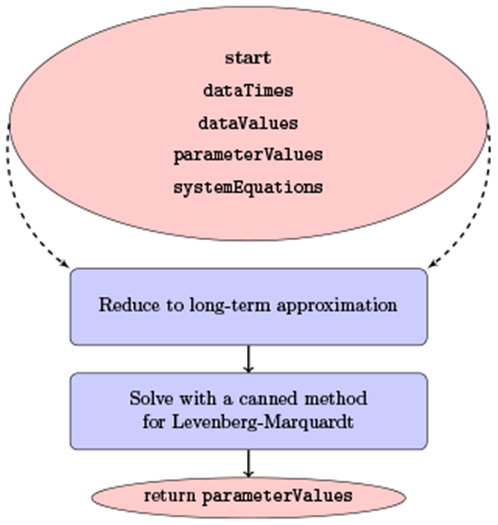
Flow diagram of the strategy with the long-term approximation. The inputs are a list of data values dataValues taken at different times dataTimes. It also requires an initial guess for the ensemble of parameters parameterValues but instead of a vector of functions, it reduces the canonical multiscale models to analytical approximations.

Fig. 6.

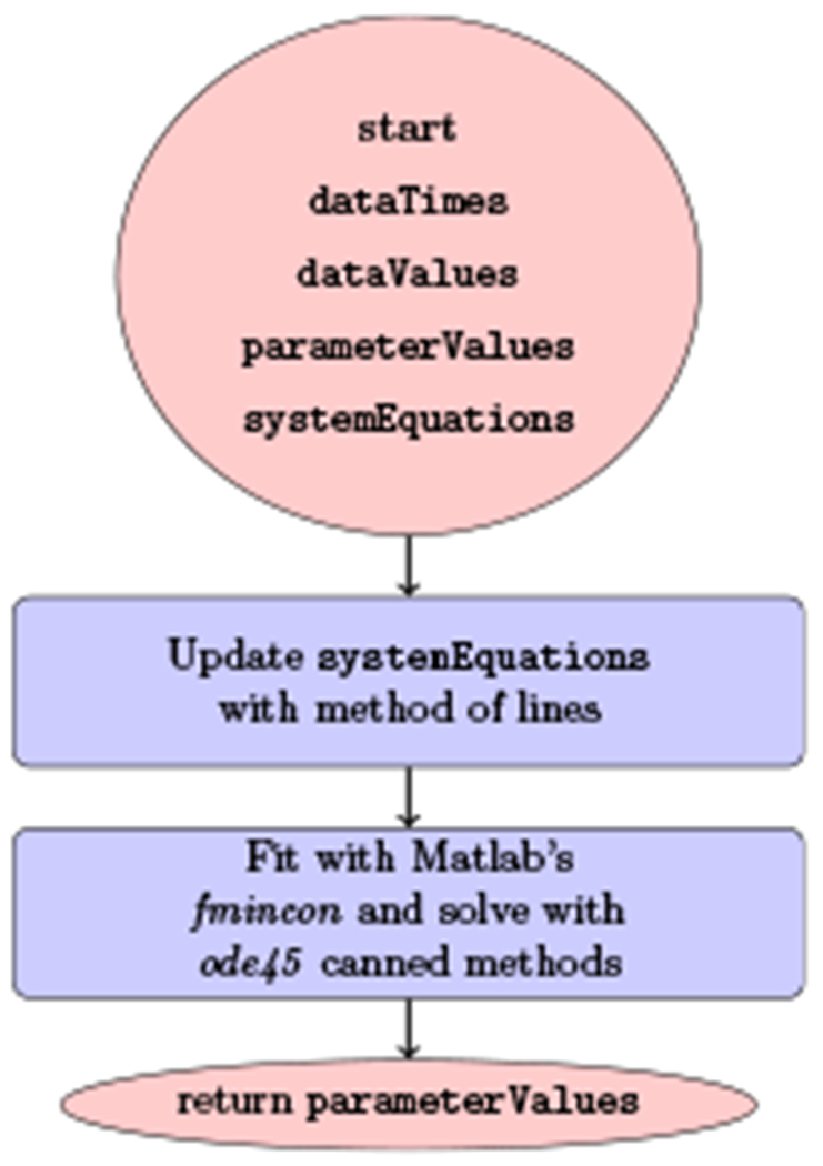
Flow diagram of the strategy using the method of lines, after which canned methods are employed with Matlab. The same list of data values dataValues, times dataTimes and an initial guess for the ensemble of parameters parameterValues are required. The system of equations this time requires an implementation of the method of lines for the PDEs and the integrals inside them.

In (Rong et al., 2013), as illustrated in Figure 5, the long-term approximation is used for the solution of the mutliscale model equations and Levenberg–Marquardt is used as a canned method. One drawback of such an approach is that it is limited to the multiscale model under treatment. In addition, the analytical approximation would change when various mutliscale models are introduced and the elaborative derivations would need to be carried for each one, with restrictions that are incorporated by the approximation being used. Finally, as discussed in the next paragraph, the use of a canned method is distancing the user away from having control over the main optimization procedure and the ability to tune it from the programming standpoint.

In (Quintela et al., 2018), a more extensive multiscale model is introduced, and a different strategy is being carried out for both the model equations solution and the parameter estimation. The model equations are solved numerically using the method of lines and Matlab’s ODE solver ode45, which implements a standard explicit 4th order Runge-Kutta. For small time steps, this is a perfectly valid approach, also it was noted in (Reinharz et al., 2018) that because of the integral in the multiscale model equations there would be no advantage in using a more sophisticated ODE solver such as Matlab’s ode23tb for stiff equations instead of ode45 for non-stiff equations. However, as was shown in (Reinharz et al., 2018), the multiscale model equations are stiff and if an increase in the time step is desired for efficiency considerations in longer time simulations, this approach remains limited in the time steps that are recommended to be taken. Moreover, for parameter estimation, the minimization procedure in (Quintela et al., 2018) is carried out with Matlab’s fmincon selecting its interior-point algorithm. While for the cases in (Quintela et al., 2018) this procedure appears successful, there are instances reported that are more problematic (e.g., https://groups.google.com/forum/#!topic/comp.soft-sys.matlab/SuNzbhEun1Y). Thus, for distributing a simulator to the community like the one that has started being developed herein, it would probably be a good practice to be able to implement protections inside the software and answer users concerns directly without relying on a black box from a third party vendor. For non-multiscale models, this would not present a problem, but for multiscale models as was demonstrated in (Reinharz et al., 2018) there is advantage in having the ability to penetrate inside the solver and optimizer routines, because of the complexity of the models.

3.4.3. Limitations of our method

The method introduced herein prepares the multiscale model equations for parameter fitting by working on them directly as an initial step. This strategy is beneficial in postponing approximations to later steps and ensuring full control of the user during the whole fitting procedure. Still, limitations exist and improvements to overcome them can be addressed in future work.

The main drawback of our method is that in its current implementation it is rather slow and may take a few hours on a parameter estimation problem with several parameters to be fitted at the same time, as in Figure 2, on a standard computer. The results in terms of the fitting performance are good but the user needs to wait patiently until the calculations are finished. Relatedly, the Rosenbrock method for the numerical solution of the multiscale model equations is an adaptive time step method. Thus, there are time steps taken in which the Rosenbrock method fluctuates just before a newer, more suitable time step is performed. Such a fluctuation has a pronounced effect during the optimization step by Levenberg-Marquardt. Without imposing a restriction to small time steps for the numerical solution of the equations, it is possible that the Backward-Differentiation Formula (BDF) would be found advantageous over the Rosenbrock method for the specific purpose of parameter fitting, a numerical solution method which will profoundly be examined in general in future work as suggested in (Reinharz et al., 2018). Additionally, the Levenberg-Marquardt method does not allow to set bounds on the parameters. This is another insight that can be exploited since we know that they must all be positives, and in the case of ε₈ and ε_α those are upper bounded by 1. To leverage this knowledge, interior-point methods have been tried and it was found that they are time consuming because of Hessian evaluations, therefore derivative-free optimization methods such as Constrained Optimization by Linear Approximation (COBYLA) should be explored in future work. Another limitation is that for each parameter introduced in future multiscale models, the derivative with respect to the new parameter needs to be taken and more equations need to be derived, as performed at the beginning of this section and in the supplementary material.

3.5. Results

Parameter estimation is a necessary procedure in all models, ranging from the biphasic model of (Neumann et al., 1998) to multiscale models (Guedj et al., 2013a; Rong et al., 2013; Rong and Perelson, 2013; Quintela et al., 2018). We present results for these two types of models worked out by a user-friendly simulator that we have developed in (Reinharz et al., 2017) for the solution of the multiscale model and extended herein towards parameter estimation for both biphasic and multiscale models. The simulator with a GUI is freely available at http://www.cs.bgu.ac.il/~dbarash/Churkin/SCE/Parameter_Estimation (with the option to either select the biphasic or the multiscale model).

3.5.1. Parameter estimation in the biphasic model

The simplest model for HCV dynamics to perform parameter estimation on is Neumann et al.’s biphasic model (Neumann et al., 1998). Although it is nonlinear, it can be solved analytically when assuming that the target cells T variable is constant. We incorporated the analytical solution to our simulator and performed parameter estimation using a nonlinear solver to solve the minimum least squares problem (Press et al., 1997) after noticing that a linear solver is insufficient. The nonlinear solver runs multiple iterations, there is a damping factor, and derivatives are calculated by varying the parameters a small amount from the previous guess. The nonlinear solver is taken from the Java least squares fitting library available at https://github.com/odinsbane/least-squares-in-java and it resembles Levenberg–Marquardt but unlike Levenberg–Marquardt, the damping is non-adaptive, which is sufficient for a good performance of parameter estimation results in this simple model. Figures 7, 8 and 9 present fitting results from three patients (Pts). Figures 6,7 correspond to Pt MBH4 who was treated with sofosbuvir combined with ledipasvir and Pt H3 who was treated with sofosbuvir with daclatasvir, respectively (Dahari et al., 2016). Figure 9 corresponds to Pt P2 who was treated with asunaprevir combined with daclatasvir (Canini et al., 2017a). A webpage with user instructions is available at http://www.cs.bgu.ac.il/~dbarash/Churkin/SCE/Parameter_Estimation/Biphasic.

Fig. 7.

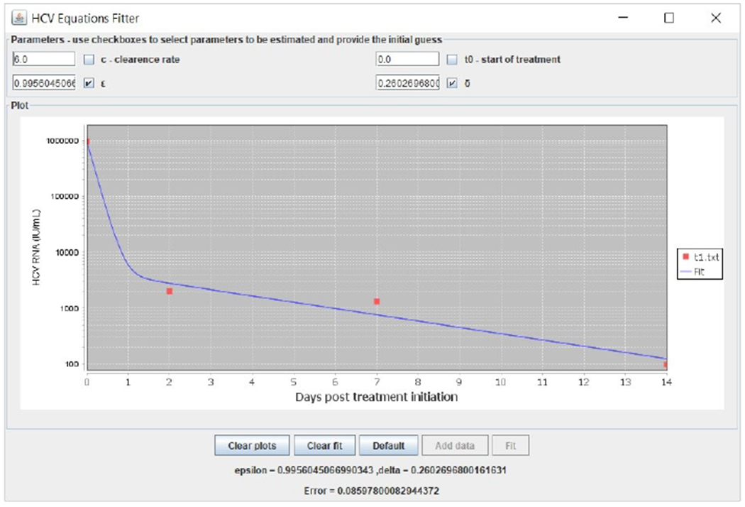
Biphasic model fitting example with data taken from (Dahari et al., 2016) of a patient who was treated with sofosbuvir combined with ledipasvir.

Fig. 8.

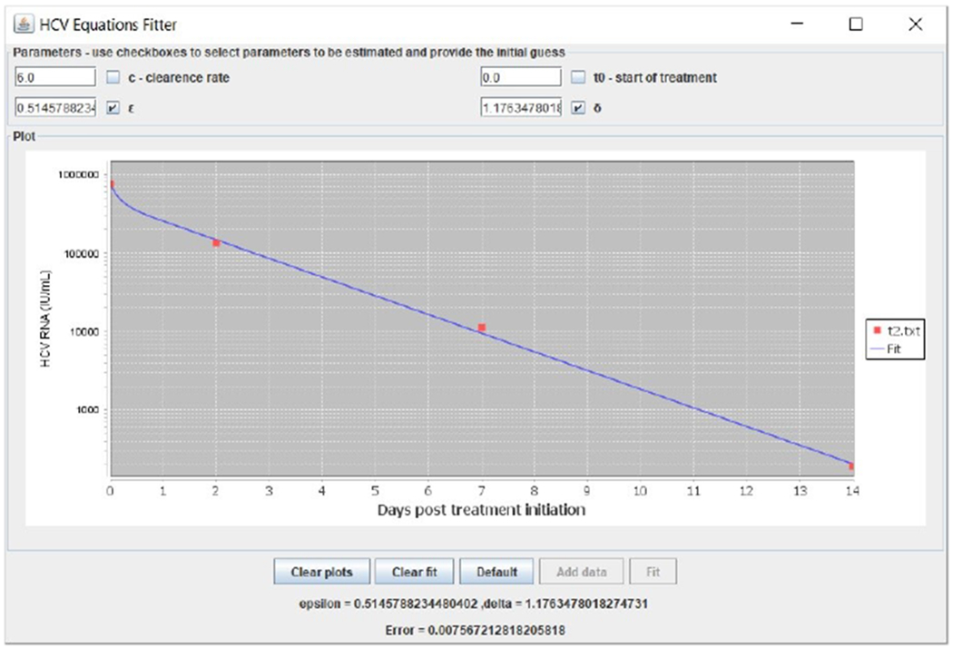
Biphasic model fitting example with data taken from (Dahari et al., 2016) of a patient who was treated with sofosbuvir combined with daclatasvir.

Fig. 9.

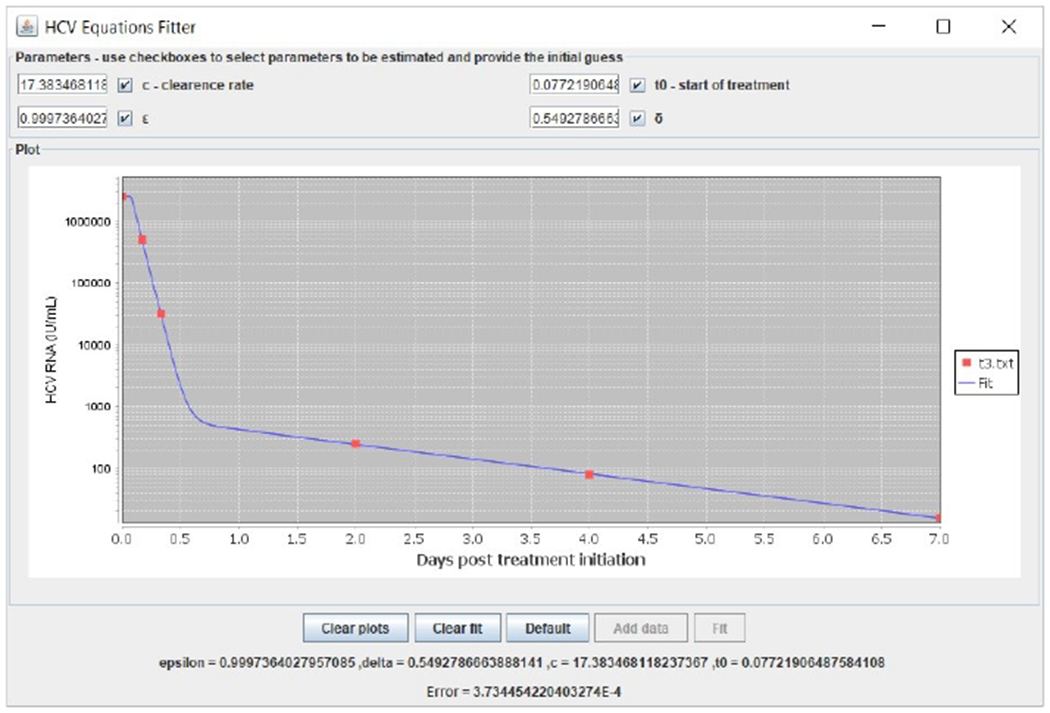
Biphasic model fitting example with data taken from (Canini et al., 2017a) of a patient who was treated with asunaprevir combined with daclatasvir.

3.5.2. Parameter estimation in the multiscale model

The multiscale model for HCV dynamics to perform parameter estimation on is taken from (Rong et al., 2013). As previously outlined and depicted in Figure 3, in our simulator we solved the model equations using the Rosenbrock method (Reinharz et al., 2017) and performed parameter estimation after preparing the derivative equations using a full implementation of the Levenberg-Marquardt without reverting to canned methods.

To illustrate the tool we provide, we first show in Figure 10 the result of fitting to generated data points from the default values the parameter ρ, when first started at 40. The predicted value of 8.152 is very close to the real value of 8.18. In Figure 11 we show the result of fitting the parameter γ, which is also worthwhile noting that it is not a parameter available in the simplified model of (Kitagawa et al., 2018). Starting from a value of 1 the result of 0.23909 is also very close to the real value of 0.24.

Fig. 10.

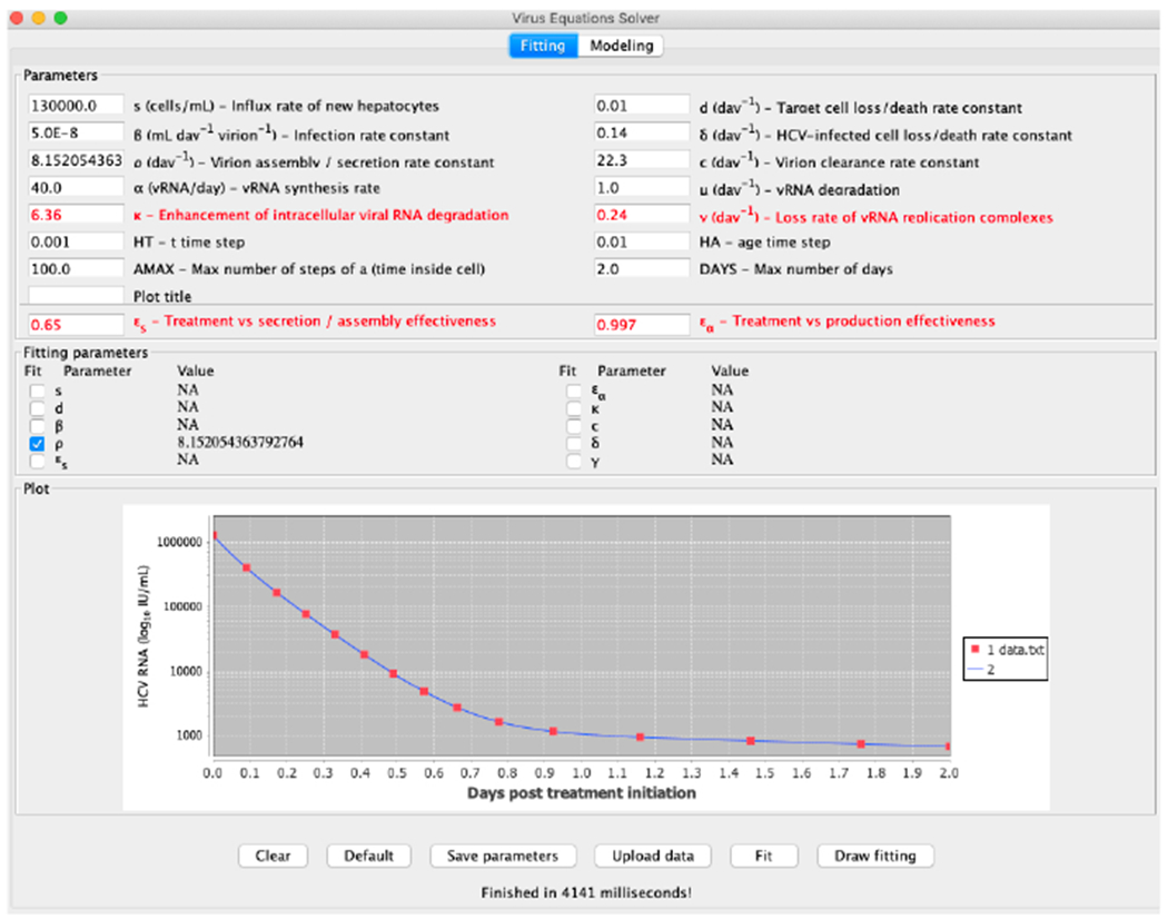
Fitting the parameter ρ to generated data points.

Fig. 11.

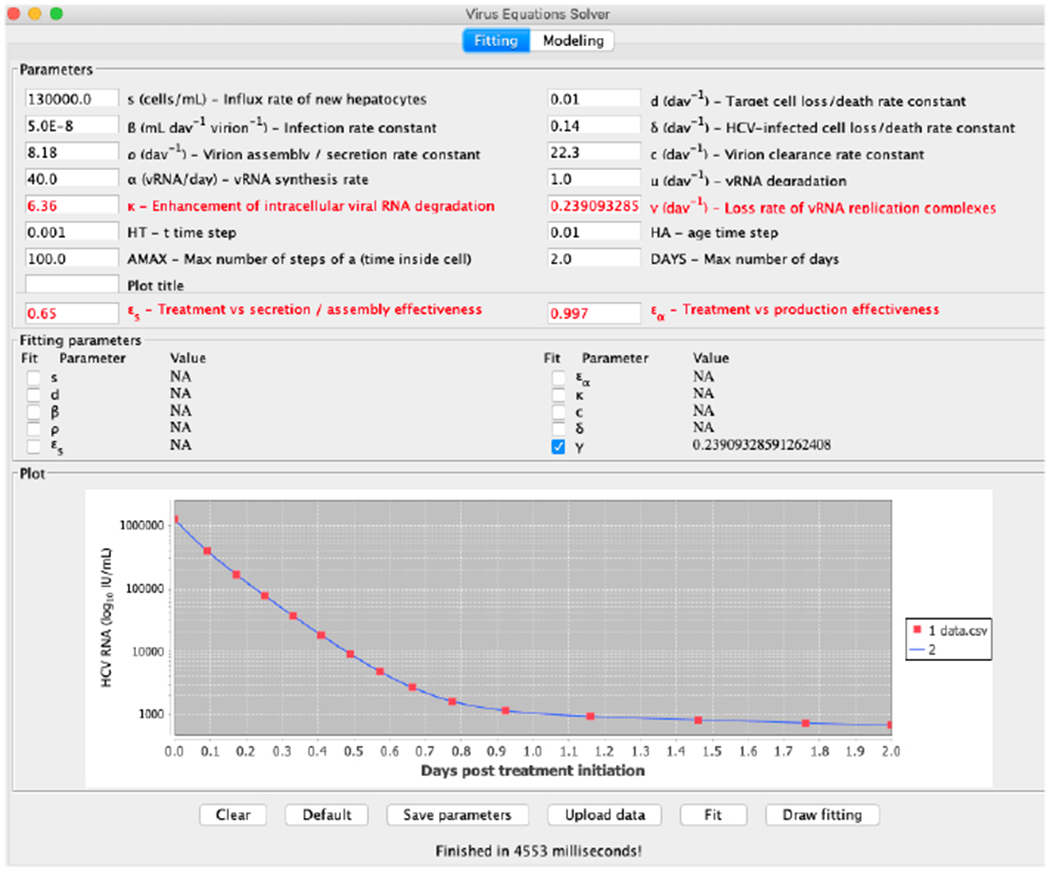
Fitting the parameter γ to generated data points.

To compare our method with the long-term approximation we fitted the four treatment parameters κ, ε_s, ε_α and γ. All the other parameters were selected with the values of Table 2. We show in Table 3 the different values of those four parameters and sum of squared-errors fitted with the two different scenarios to the data emanating from a patient. We also show in parenthesis the standard deviations. In the leftmost column we fitted the long-term approximation with the retrieved data points using the scipy.optimize.curve_fit method, which is a Python implementation of a simple Levenberg-Marquardt scheme as a canned method. In the rightmost column are the values obtained by our method.

Table 3.

Values of the parameters when fitted to the patient digitized data, standard deviation shown between parenthesis. The long-term column has the values when the retrieved data points are fitted to the long-term approximation equation. The rightmost column contains the fitted parameters values by our method, which combines the Levenberg–Marquardt and Rosenbrock numerical schemes. The fixed parameters have the values shown in Table 2.

	Long-term approximation	Rosenbrock+Levenberg–Marquardt
εs	0.60 (0.198)	0.60 (0.992)
εα	0.994 (0.002)	0.994 (0.009)
κ	6.16 (0.947)	6.218 (4.640)
γ(d−1)	0.14 (0.039)	0.139 (0.178)
sum error2	0.53	0.51

For comparison of the results between the line fit when the retrieved data points are fitted to the long-term approximation equation and our method, we compute the sum of squares of the errors for each data point. It is shown that our method achieved slightly better results. To further illustrate the tool we provide, we show in Figure 12 the starting configuration after the data was inserted as input and in Figure 13 the final result. In Figure 14 we present the same curve compared with the line fit of the long term approximation, as in Table 3. A webpage with user instructions is available at http://www.cs.bgu.ac.il/~dbarash/Churkin/SCE/Parameter_Estimation/Multiscale.

Fig. 12.

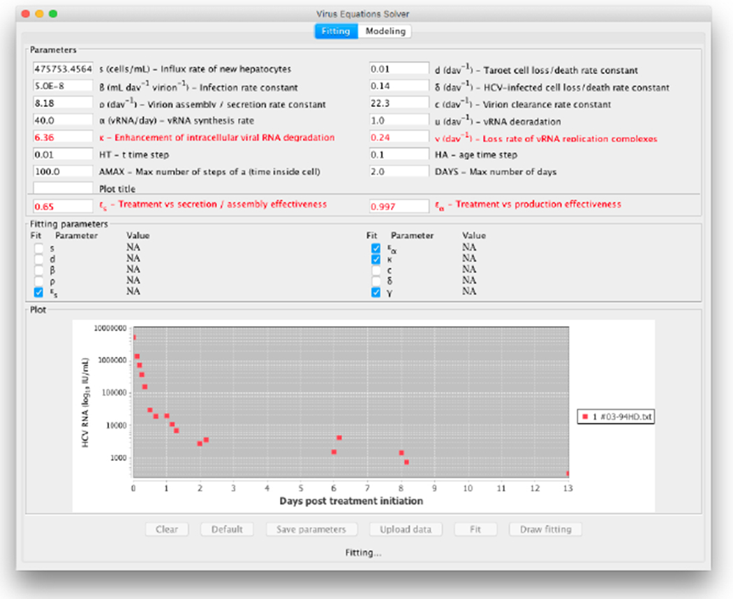
Start fit that emanates from data of a patient reported in (Rong et al., 2013)

Fig. 13.

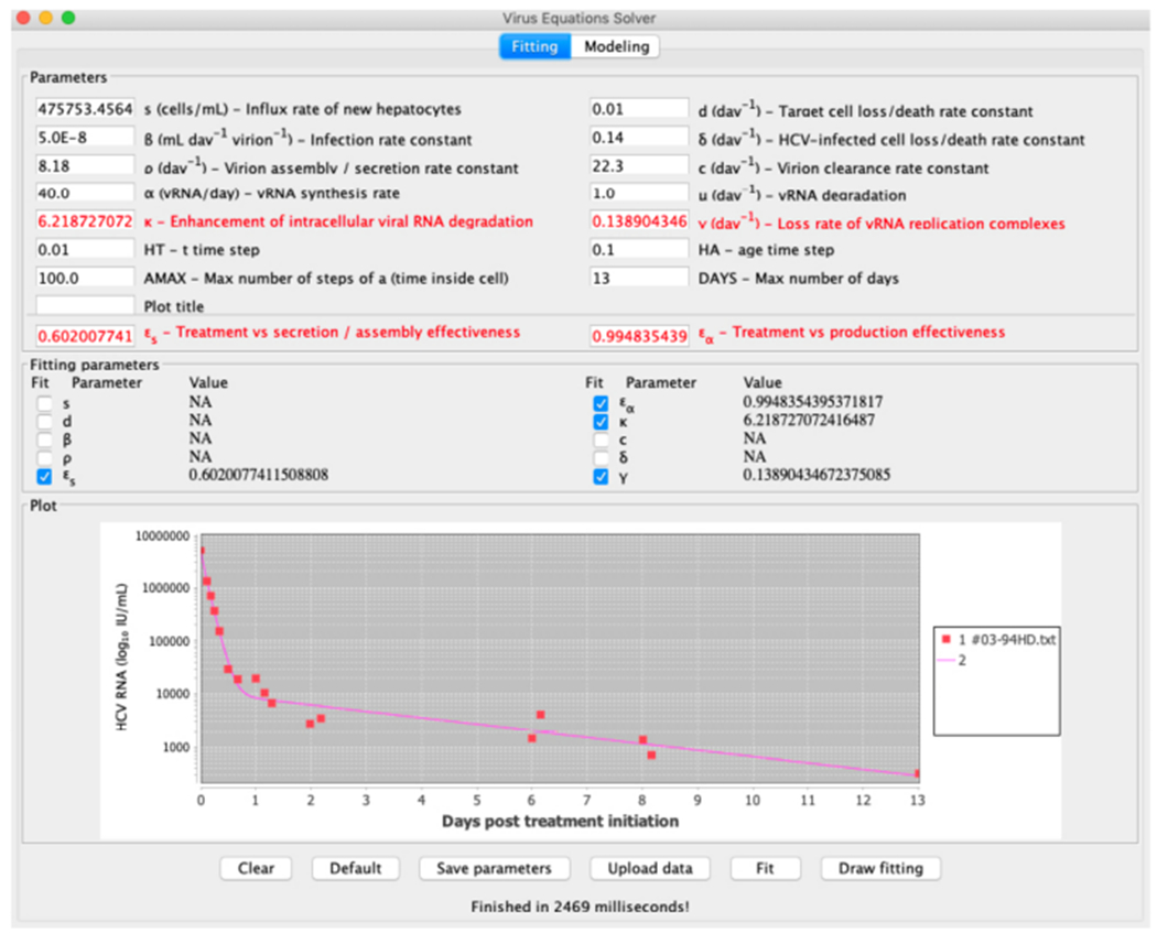
End fit that emanates from data of a patient reported in (Rong et al., 2013)

Fig. 14.

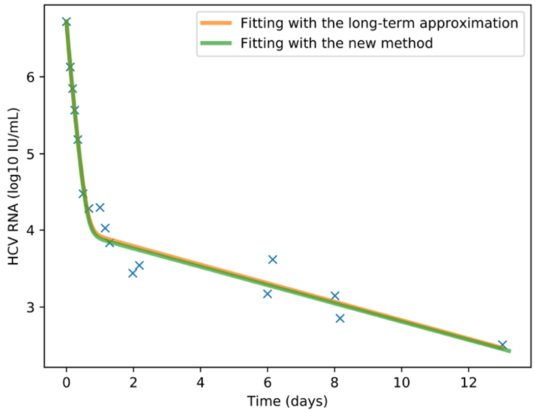
Comparison between the line fits of the long-term approximation and our method on the retrieved data points that are shown.

4. Concluding Remarks

Parameter estimation is a challenging problem for mathematical models that are based on differential equations. In the context of viral dynamic models, even a simple model such as the biphasic model (Neumann et al., 1998) requires a nonlinear method for the least squares minimization because a linear method is not sufficient, as was experimented by us and demonstrated with our simulator for the biphasic model in the Results section. The development of more complicated models such as viral dynamic models that consider intracellular viral RNA replication, namely age-structured PDE multiscale models to study viral hepatitis dynamics during antiviral therapy (Rong et al., 2013; Rong and Perelson, 2013; Guedj et al., 2013a; Quintela et al., 2018), presents a need for more sophisticated strategies that perform parameter estimation while solving the model equations simultaneously. Simply transforming the PDE multiscale models to a set of ODEs (Kitagawa et al., 2018), while possibly having other merits, requires a change in the parameters and therefore does not offer a comprehensive solution to the problem.

From the parameter estimation standpoint, as previously outlined, multiscale models are considerably more challenging than the biphasic model. Not only that conducting a search in at least a 10-parameter search space is more difficult than in a 4-parameter search space, also the task of solving the model equations themselves and how to connect the equations solution to the optimization procedure requires more sophistication. Previously, this was approached in (Rong et al., 2013) by using the long-term approximation along with a canned method for Levenberg-Marquardt, and in (Quintela et al., 2018) by the method of lines and then employing Matlab’s 4th order Runge-Kutta solver along with a canned method available in Matlab called fmincon for the optimization. While these strategies work sufficiently well for specific cases, because of their use of canned methods they are problematic from the standpoint of the user’s capability to access and control them. Thus far, no source code has been released free of charge for the benefit of the community and while these strategies were described coherently in the context of presenting multiscale models, they were not intended to provide to the user a comprehensive solution of their own. It requires considerable implementation efforts by the user (e.g., in reading documentation about Matlab’s fmincon after purchasing a license to use the Optimization Toolbox). There is clearly a need to provide the user with a free of charge simulator that is effortless to operate and a code that can be accessed for dissemination and future development.

The strategy we presented herein requires no canned methods utilization. It works directly on the multiscale model equations, preparing them in advance for the optimization procedure by taking their derivatives with respect to the parameters, in contrast to solving them first by an analytical approximation or performing the method of lines as a first step. For the solution of the model equations, the Rosenbrock method described in (Reinharz et al., 2017) is employed, as was shown to be advantageous in comparison to other solution schemes in (Reinharz et al., 2018). For the optimization procedure, Levenberg–Marquardt is employed in full (not as a canned method) such that the user has access to the source code at each point in the procedure. The whole method is provided in a form of a multiscale model simulator with a user-friendly GUI.

The method is rather slow in most scenarios, which may take several hours or more to reach the desired solution on a standard computer. Nevertheless, fitting at once the four parameters κ, ε_s, ε_α and γ yields good results and can be computed in less than a day. Future work will be devoted to improve these limitations. To date, this is the first time that a parameter estimation method for multiscale models is distributed free of charge with its source code to the community within a user-friendly tool, which by itself will be helpful to practitioners. The new method is based on flexible components that can be easily accessed and modified by developers who are interested in other research modeling areas such as the dynamics of a viral population over both space and time (e.g., modeling spatial aspects of within-host viral spread (Gallagher et al., 2018; Kumberger et al., 2018)). The method can be generalized with regards to the outlined model parameters, such as ρ, δ, and α, which can be made dependent on the age a. For example, we can utilize our method when the constant production rate α is replaced by an age-dependent logistic function. The method is also achieving convincing results as was demonstrated herein in comparison to other strategies and will be beneficial among the arsenal of methods that were developed for parameter estimation in multiscale models.

Appendix

In this appendix we briefly show the derivation of the equations that constitute a preparatory step before the optimization procedure for the other seven parameters that were not included in the main text (three were already shown starting from Section 3.3.1). For more details the interested reader is referred to Section 3.3.1).

Parameter d :

The derivative of the general function f (the vector [T, V]) with respect to d is:

$$\frac{\partial f}{\partial d}\left(t,y^d\right)=\left[-T-d\frac{\partial T}{\partial d}-\beta \left(\frac{\partial V}{\partial d}T+V\frac{\partial T}{\partial d}\right)\left(1-{\epsilon }_s\right){\int }_0^{\infty }\rho R\left(a,t\right)\frac{\partial I}{\partial d}\left(a,t\right)\text{d}a-c\frac{\partial V}{\partial d}\right]$$

where $y^d=\{\begin{array}{c}T\\ V\\ \frac{\partial T}{\partial d}\\ \frac{\partial V}{\partial d}\end{array}$.

Furthermore:

$$\frac{\partial R\left(a,t\right)}{\partial d}=0,$$

$$\frac{\partial \stackrel{\_}{T}}{\partial d}=0,$$

$$\frac{\partial \stackrel{\_}{V}}{\partial d}=-1/\beta ,$$

$$\frac{\partial I\left(a,t\right)}{\partial d}=\{\begin{array}{ll}\beta \left(\frac{\partial V}{\partial d}\left(t-a\right)T\left(t-a\right)+V\left(t-a\right)\frac{\partial T}{\partial d}\left(t-a\right)\right){\text{e}}^{-\delta a}& a<t\\ -c/\left(\beta N\right){\text{e}}^{-\delta a}& a>t\end{array},$$

The upper right block matrix of the Jacobian is:

$$f_{d,2\times 2}^{\prime }=\left(\begin{array}{cc}0& 0\\ \left(1-{\epsilon }_s\right){\int }_0^t\rho R\left(a,t\right)\times \frac{\partial I\left(a,t\right)}{\partial \frac{\partial T}{\partial d}}\text{d}a& \left(1-{\epsilon }_s\right){\int }_0^t\rho R\left(a,t\right)\times \frac{\partial I\left(a,t\right)}{\partial \frac{\partial V}{\partial d}}\text{d}a\end{array}\right)$$

and the transposed last two rows of the Jacobian are:

$$\left({\left(f_{d,3}^{\prime }\right)}^{\mathrm{tr}},{\left(f_{d,4}^{\prime }\right)}^{\mathrm{tr}}\right):=\left(\begin{array}{ll}-1-\beta \frac{\partial V}{\partial d}& \left(1-{\epsilon }_s\right){\int }_0^t\rho R\left(a,t\right)\frac{\partial \frac{\partial I\left(a,t\right)}{\partial d}}{\partial T}\text{d}a\\ -\beta \frac{\partial T}{\partial d}& \left(1-{\epsilon }_s\right){\int }_0^t\rho R\left(a,t\right)\frac{\partial \frac{\partial I\left(a,t\right)}{\partial d}}{\partial V}\text{d}a\\ -d-\beta V& \left(1-{\epsilon }_s\right){\int }_0^t\rho R\left(a,t\right)\frac{\partial \frac{\partial I\left(a,t\right)}{\partial d}}{\partial \frac{\partial T}{\partial d}}\text{d}a\\ -\beta T& \left(1-{\epsilon }_s\right){\int }_0^t\rho R\left(a,t\right)\frac{\partial \frac{\partial I\left(a,t\right)}{\partial d}}{\partial \frac{\partial V}{\partial d}}\text{d}a-c\end{array}\right),$$

$$\frac{\partial \frac{\partial f}{\partial d}}{\partial t}=\left[0,\left(1-{\epsilon }_s\right){\int }_0^{\infty }\rho \left(\frac{\partial R\left(a,t\right)}{\partial t}\frac{\partial I}{\partial d}\left(a,t\right)+R\left(a,t\right)\frac{\partial \frac{\partial I\left(a,t\right)}{\partial d}}{\partial t}\right)\text{d}a\right].$$

Parameter β:

The derivative of the general function f (the vector [T, V]) with respect to β is:

$$\begin{gathered} \frac{\partial f}{\partial \beta }\left(t,y^{\beta }\right)=[-d\frac{\partial T}{\partial \beta }-\left(VT+\beta \frac{\partial V}{\partial \beta }T+\beta V\frac{\partial T}{\partial \beta }\right) \\ \left(1-{\epsilon }_s\right){\int }_0^{\infty }\rho R\left(a,t\right)\frac{\partial I\left(a,t\right)}{\partial \beta }\text{d}a-c\frac{\partial V}{\partial \beta }] \end{gathered}$$

where $y^{\beta }=\{\begin{array}{c}T\\ V\\ \frac{\partial T}{\partial \beta }\\ \frac{\partial V}{\partial \beta }\end{array}$.

Furthermore:

$$\frac{\partial R\left(a,t\right)}{\partial \beta }=0,$$

$$\frac{\partial \stackrel{\_}{T}}{\partial \beta }=-c/\left({\beta }^{2}N\right),$$

$$\frac{\partial \stackrel{\_}{V}}{\partial \beta }=d/{\beta }^2,$$

$$\frac{\partial I\left(a,t\right)}{\partial \beta }=\{\begin{array}{ll}\left(V\left(t-a\right)T\left(t-a\right)+\beta \frac{\partial V}{\partial \beta }\left(t-a\right)T\left(t-a\right)+\beta V\left(t-a\right)\frac{\partial T}{\partial \beta }\left(t-a\right)\right){\text{e}}^{-\delta a}& a<t\\ dc/\left({\beta }^{2}N\right){\text{e}}^{-\delta a}& a>t\end{array},$$

The upper right block matrix of the Jacobian is:

$$f_{\beta ,2\times 2}^{\prime }=\left(\begin{array}{cc}0& 0\\ \left(1-{\epsilon }_s\right){\int }_0^t\rho R\left(a,t\right)\times \frac{\partial I\left(a,t\right)}{\partial \frac{\partial T}{\partial \beta }}\text{d}a& \left(1-{\epsilon }_s\right){\int }_0^t\rho R\left(a,t\right)\times \frac{\partial I\left(a,t\right)}{\partial \frac{\partial V}{\partial \beta }}\text{d}a\end{array}\right)$$

and the transposed last two rows of the Jacobian are:

$$\left({\left(f_{\beta ,3}^{\prime }\right)}^{\mathrm{tr}},{\left(f_{\beta ,4}^{\prime }\right)}^{\mathrm{tr}}\right):=\left(\begin{array}{ll}-\left(V+\beta \frac{\partial V}{\partial \beta }\right)& \left(1-{\epsilon }_s\right){\int }_0^t\rho R\left(a,t\right)\frac{\partial \frac{\partial I\left(a,t\right)}{\partial \beta }}{\partial T}\text{d}a\\ -\left(T+\beta \frac{\partial T}{\partial \beta }\right)& \left(1-{\epsilon }_s\right){\int }_0^t\rho R\left(a,t\right)\frac{\partial \frac{\partial I\left(a,t\right)}{\partial \beta }}{\partial V}\text{d}a\\ -d-\beta V& \left(1-{\epsilon }_s\right){\int }_0^t\rho R\left(a,t\right)\frac{\partial \frac{\partial I\left(a,t\right)}{\partial \beta }}{\partial \frac{\partial T}{\partial \beta }}\text{d}a\\ -\beta T& \left(1-{\epsilon }_s\right){\int }_0^t\rho R\left(a,t\right)\frac{\partial \frac{\partial I\left(a,t\right)}{\partial \beta }}{\partial \frac{\partial V}{\partial \beta }}\text{d}a-c\end{array}\right),$$

$$\frac{\partial \frac{\partial f}{\partial \beta }}{\partial t}=\left[0,\left(1-{\epsilon }_s\right){\int }_0^{\infty }\rho \left(\frac{\partial R\left(a,t\right)}{\partial t}\frac{\partial I}{\partial \beta }\left(a,t\right)+R\left(a,t\right)\frac{\partial \frac{\partial I\left(a,t\right)}{\partial \beta }}{\partial t}\right)\text{d}a\right].$$

Parameter ε_s:

The derivative of the general function f (the vector [T, V]) with respect to ε_s is:

$$\frac{\partial f}{\partial {\epsilon }_s}\left(t,y^{{\epsilon }_s}\right)=[-d\frac{\partial T}{\partial {\epsilon }_s}-\beta \left(\frac{\partial V}{\partial {\epsilon }_s}T+V\frac{\partial T}{\partial {\epsilon }_s}\right),-{\int }_0^{\infty }\rho R\left(a,t\right)I\left(a,t\right)\text{d}a+\left(1-{\epsilon }_s\right){\int }_0^{\infty }\rho \frac{\partial R\left(a,t\right)}{\partial {\epsilon }_s}I\left(a,t\right)\text{d}a+\left(1-{\epsilon }_s\right){\int }_0^t\rho R\left(a,t\right)\frac{\partial I}{\partial {\epsilon }_s}\left(a,t\right)\text{d}a-c\frac{\partial V}{\partial {\epsilon }_s}]$$

where $y^{{\epsilon }_s}=\{\begin{array}{c}T\\ V\\ \frac{\partial T}{\partial {\epsilon }_s}\\ \frac{\partial V}{\partial {\epsilon }_s}\end{array}$.

Furthermore:

$$\begin{gathered} \frac{\partial R\left(a,t\right)}{\partial {\epsilon }_s}=\{\begin{array}{ll}\rho \frac{\left(1-{\epsilon }_{\alpha }\right)\alpha {\text{e}}^{-\gamma t}}{{\left(\left(1-{\epsilon }_s\right)\rho +\kappa \mu -\gamma \right)}^2} \\ -\rho \frac{\left(1-{\epsilon }_{\alpha }\right)\alpha {\text{e}}^{-\gamma \left(t-a\right)}}{{\left(\left(1-{\epsilon }_s\right)\rho +\kappa \mu -\gamma \right)}^2}{\text{e}}^{-\left(\left(1-{\epsilon }_s\right)\rho +\kappa \mu \right)a} \\ +\rho a\left(1-\frac{\left(1-{\epsilon }_{\alpha }\right)\alpha {\text{e}}^{-\gamma \left(t-a\right)}}{\left(1-{\epsilon }_s\right)\rho +\kappa \mu -\gamma }\right){\text{e}}^{-\left(\left(1-{\epsilon }_s\right)\rho +\kappa \mu \right)a}& a<t\\ \rho \frac{\left(1-{\epsilon }_{\alpha }\right)\alpha {\text{e}}^{-\gamma t}}{{\left(\left(1-{\epsilon }_s\right)\rho +\kappa \mu -\gamma \right)}^2} \\ -\rho \frac{\left(1-{\epsilon }_{\alpha }\right)\alpha }{{\left(\left(1-{\epsilon }_s\right)\rho +\kappa \mu -\gamma \right)}^2}{\text{e}}^{-\left(\left(1-{\epsilon }_s\right)\rho +\kappa \mu \right)t} \\ +\rho t\left(\frac{\alpha }{\rho +\mu }+\left(1-\frac{\alpha }{\rho +\mu }\right){\text{e}}^{-\left(\rho +\mu \right)\left(a-t\right)}-\frac{\left(1-{\epsilon }_{\alpha }\right)\alpha }{\left(1-{\epsilon }_s\right)\rho +\kappa \mu -\gamma }\right){\text{e}}^{-\left(\left(1-{\epsilon }_s\right)\rho +\kappa \mu \right)t}& a>t\end{array}, \end{gathered}$$

$$\frac{\partial \overline{T}}{\partial {\epsilon }_s}=0,$$

$$\frac{\partial \overline{V}}{\partial {\epsilon }_s}=0,$$

$$\frac{\partial I(a,t)}{\partial {\epsilon }_s}=\{\begin{array}{ll}\beta \left(\frac{\partial V}{\partial {\epsilon }_s}\left(t-a\right)T\left(t-a\right)+V\left(t-a\right)\frac{\partial T}{\partial {\epsilon }_s}\left(t-a\right)\right){\text{e}}^{-\delta a}& a<t\\ 0& a>t\end{array},$$

The upper right block matrix of the Jacobian is:

$$f_{{\epsilon }_s,2\times 2}^{\prime }=\left(\begin{array}{cc}0& 0\\ \left(1-{\epsilon }_s\right){\int }_0^t\rho R\left(a,t\right)\times \frac{\partial I\left(a,t\right)}{\partial \frac{\partial T}{\partial {\epsilon }_s}}\text{d}a& \left(1-{\epsilon }_s\right){\int }_0^t\rho R\left(a,t\right)\times \frac{\partial I\left(a,t\right)}{\partial \frac{\partial V}{\partial {\epsilon }_s}}\text{d}a\end{array}\right)$$

and the transposed last two rows of the Jacobian are:

$$\left({\left(f_{{\epsilon }_s,3}^{\prime }\right)}^{\mathrm{tr}},{\left(f_{{\epsilon }_s,4}^{\prime }\right)}^{\mathrm{tr}}\right):=\left(\begin{array}{ll}-\beta \frac{\partial V}{\partial {\epsilon }_s}& -{\int }_0^t\rho R\left(a,t\right)\frac{\partial I\left(a,t\right)}{\partial T}\text{d}a+\left(1-{\epsilon }_s\right){\int }_0^t\rho \frac{\partial R\left(a,t\right)}{\partial {\epsilon }_s}\frac{\partial I\left(a,t\right)}{\partial T}\text{d}a+\left(1-{\epsilon }_s\right){\int }_0^t\rho R\left(a,t\right)\frac{\partial \frac{\partial I\left(a,t\right)}{\partial {\epsilon }_s}}{\partial T}\text{d}a\\ -\beta \frac{\partial T}{\partial {\epsilon }_s}& -{\int }_0^t\rho R\left(a,t\right)\frac{\partial I\left(a,t\right)}{\partial V}\text{d}a+\left(1-{\epsilon }_s\right){\int }_0^t\rho \frac{\partial R\left(a,t\right)}{\partial {\epsilon }_s}\frac{\partial I\left(a,t\right)}{\partial V}\text{d}a+\left(1-{\epsilon }_s\right){\int }_0^t\rho R\left(a,t\right)\frac{\partial \frac{\partial I\left(a,t\right)}{\partial {\epsilon }_s}}{\partial V}\text{d}a\\ -d-\beta V& -{\int }_0^t\rho R\left(a,t\right)\frac{\partial I\left(a,t\right)}{\partial \frac{\partial T}{\partial {\epsilon }_s}}\text{d}a+\left(1-{\epsilon }_s\right){\int }_0^t\rho \frac{\partial R\left(a,t\right)}{\partial {\epsilon }_s}\frac{\partial I\left(a,t\right)}{\partial \frac{\partial T}{\partial {\epsilon }_s}}\text{d}a+\left(1-{\epsilon }_s\right){\int }_0^t\rho R\left(a,t\right)\frac{\partial \frac{\partial I\left(a,t\right)}{\partial {\epsilon }_s}}{\partial \frac{\partial T}{\partial {\epsilon }_s}}\text{d}a\\ -\beta T& -{\int }_0^t\rho R\left(a,t\right)\frac{\partial I\left(a,t\right)}{\partial \frac{\partial V}{\partial {\epsilon }_s}}\text{d}a+\left(1-{\epsilon }_s\right){\int }_0^t\rho \frac{\partial R\left(a,t\right)}{\partial {\epsilon }_s}\frac{\partial I\left(a,t\right)}{\partial \frac{\partial V}{\partial {\epsilon }_s}}\text{d}a+\left(1-{\epsilon }_s\right){\int }_0^t\rho R\left(a,t\right)\frac{\partial \frac{\partial I\left(a,t\right)}{\partial {\epsilon }_s}}{\partial \frac{\partial V}{\partial {\epsilon }_s}}\text{d}a-c\end{array}\right),$$

$$\frac{\partial \frac{\partial f}{\partial {\epsilon }_s}}{\partial t}=[0,-{\int }_0^{\infty }\rho \left(\frac{\partial R\left(a,t\right)}{\partial t}I\left(a,t\right)+R\left(a,t\right)\frac{\partial I\left(a,t\right)}{\partial t}\right)\text{d}a+\left(1-{\epsilon }_s\right){\int }_0^{\infty }\rho \left(\frac{\partial \frac{\partial R\left(a,t\right)}{\partial {\epsilon }_s}}{\partial t}I\left(a,t\right)+\frac{\partial R\left(a,t\right)}{\partial {\epsilon }_s}\frac{\partial I\left(a,t\right)}{\partial t}\right)\text{d}a+\left(1-{\epsilon }_s\right){\int }_0^t\rho \left(\frac{\partial R\left(a,t\right)}{\partial t},\frac{\partial I\left(a,t\right)}{\partial {\epsilon }_s}+R\left(a,t\right)\frac{\partial \frac{\partial I\left(a,t\right)}{\partial {\epsilon }_s}}{\partial t}\right)\text{d}a]$$

where:

$$\begin{gathered} \frac{\partial \frac{\partial R\left(a,t\right)}{\partial {\epsilon }_s}}{\partial t}=\{\begin{array}{ll}-\gamma \rho \frac{\left(1-{\epsilon }_{\alpha }\right)\alpha {\text{e}}^{-\gamma t}}{{\left(\left(1-{\epsilon }_s\right)\rho +\kappa \mu -\gamma \right)}^2} \\ +\gamma \rho \frac{\left(1-{\epsilon }_{\alpha }\right)\alpha {\text{e}}^{-\gamma \left(t-a\right)}}{{\left(\left(1-{\epsilon }_s\right)\rho +\kappa \mu -\gamma \right)}^2}{\text{e}}^{-\left(\left(1-{\epsilon }_s\right)\rho +\kappa \mu \right)a} \\ +\gamma \rho a\frac{\left(1-{\epsilon }_{\alpha }\right)\alpha {\text{e}}^{-\gamma \left(t-a\right)}}{\left(1-{\epsilon }_s\right)\rho +\kappa \mu -\gamma }{\text{e}}^{-\left(\left(1-{\epsilon }_s\right)\rho +\kappa \mu \right)a}& a<t\\ -\gamma \rho \frac{\left(1-{\epsilon }_{\alpha }\right)\alpha {\text{e}}^{-\gamma t}}{{\left(\left(1-{\epsilon }_s\right)\rho +\kappa \mu -\gamma \right)}^2} \\ +\left(\left(1-{\epsilon }_s\right)\rho +\kappa \mu \right)\rho \frac{\left(1-{\epsilon }_{\alpha }\right)\alpha }{{\left(\left(1-{\epsilon }_s\right)\rho +\kappa \mu -\gamma \right)}^2}{\text{e}}^{-\left(\left(1-{\epsilon }_s\right)\rho +\kappa \mu \right)t} \\ +\rho \left(\frac{\alpha }{\rho +\mu }+\left(1-\frac{\alpha }{\rho +\mu }\right){\text{e}}^{-\left(\rho +\mu \right)\left(a-t\right)}-\frac{\left(1-{\epsilon }_{\alpha }\right)\alpha }{\left(1-{\epsilon }_s\right)\rho +\kappa \mu -\gamma }\right){\text{e}}^{-\left(\left(1-{\epsilon }_s\right)\rho +\kappa \mu \right)t} \\ +\left(\rho +\mu \right)\rho t\left(1-\frac{\alpha }{\rho +\mu }\right){\text{e}}^{-\left(\rho +\mu \right)\left(a-t\right)}{\text{e}}^{-\left(\left(1-{\epsilon }_s\right)\rho +\kappa \mu \right)t} \\ +\left(\left(1-{\epsilon }_s\right)\rho +\kappa \mu \right)\rho t\left(\frac{\alpha }{\rho +\mu }+\left(1-\frac{\alpha }{\rho +\mu }\right){\text{e}}^{-\left(\rho +\mu \right)\left(a-t\right)}-\frac{\left(1-{\epsilon }_{\alpha }\right)\alpha }{\left(1-{\epsilon }_s\right)\rho +\kappa \mu -\gamma }\right) \\ \times {\text{e}}^{-\left(\left(1-{\epsilon }_s\right)\rho +\kappa \mu \right)t}& a>t\end{array}. \end{gathered}$$

Parameter ε_α:

The derivative of the general function f (the vector [T, V]) with respect to ε_α is:

$$\frac{\partial f}{\partial {\epsilon }_{\alpha }}\left(t,y^{{\epsilon }_{\alpha }}\right)=[-d\frac{\partial T}{\partial {\epsilon }_{\alpha }}-\beta \left(\frac{\partial V}{\partial {\epsilon }_{\alpha }}T+V\frac{\partial T}{\partial {\epsilon }_{\alpha }}\right),\left(1-{\epsilon }_s\right){\int }_0^{\infty }\rho \frac{\partial R\left(a,t\right)}{\partial {\epsilon }_{\alpha }}I\left(a,t\right)\text{d}a+\left(1-{\epsilon }_s\right){\int }_0^t\rho R\left(a,t\right)\frac{\partial I}{\partial {\epsilon }_{\alpha }}\left(a,t\right)\text{d}a-c\frac{\partial V}{\partial {\epsilon }_{\alpha }}]$$

where $y^{{\epsilon }_{\alpha }}=\{\begin{array}{c}T\\ V\\ \frac{\partial T}{\partial {\epsilon }_{\alpha }}\\ \frac{\partial V}{\partial {\epsilon }_{\alpha }}\end{array}$.

Furthermore:

$$\frac{\partial R\left(a,t\right)}{\partial {\epsilon }_{\alpha }}=\{\begin{array}{cc}-\frac{\alpha {\text{e}}^{-\gamma t}}{\left(1-{\epsilon }_s\right)\rho +\kappa \mu -\gamma }+\frac{\alpha {\text{e}}^{-\gamma \left(t-a\right)}}{\left(1-{\epsilon }_s\right)\rho +\kappa \mu -\gamma }{\text{e}}^{-\left(\left(1-{\epsilon }_s\right)\rho +\kappa \mu \right)a}& a<t\\ -\frac{\alpha {\text{e}}^{-\gamma t}}{\left(1-{\epsilon }_s\right)\rho +\kappa \mu -\gamma }+\frac{\alpha }{\left(1-{\epsilon }_s\right)\rho +\kappa \mu -\gamma }{\text{e}}^{-\left(\left(1-{\epsilon }_s\right)\rho +\kappa \mu \right)t}& a>t\end{array},$$

$$\frac{\partial \stackrel{\_}{T}}{\partial {\epsilon }_{\alpha }}=0,$$

$$\frac{\partial \stackrel{\_}{V}}{\partial {\epsilon }_{\alpha }}=0,$$

$$\frac{\partial I\left(a,t\right)}{\partial {\epsilon }_{\alpha }}=\{\begin{array}{ll}\beta \left(\frac{\partial V}{\partial {\epsilon }_{\alpha }}\left(t-a\right)T\left(t-a\right)+V\left(t-a\right)\frac{\partial T}{\partial {\epsilon }_{\alpha }}\left(t-a\right)\right){\text{e}}^{-\delta a}& a<t\\ 0& a>t\end{array},$$

The upper right block matrix of the Jacobian is:

$$f_{{\epsilon }_{\alpha },2\times 2}^{\prime }=\left(\begin{array}{cc}0& 0\\ \left(1-{\epsilon }_s\right){\int }_0^t\rho R\left(a,t\right)\times \frac{\partial I\left(a,t\right)}{\partial \frac{\partial T}{\partial {\epsilon }_{\alpha }}}\text{d}a& \left(1-{\epsilon }_s\right){\int }_0^t\rho R\left(a,t\right)\times \frac{\partial I\left(a,t\right)}{\partial \frac{\partial V}{\partial {\epsilon }_{\alpha }}}\text{d}a\end{array}\right)$$

and the transposed last two rows of the Jacobian are:

$$\left({\left(f_{{\epsilon }_{\alpha },3}^{\prime }\right)}^{\mathrm{tr}},{\left(f_{{\epsilon }_{\alpha },4}^{\prime }\right)}^{\mathrm{tr}}\right):=\left(\begin{array}{ll}-\beta \frac{\partial V}{\partial {\epsilon }_{\alpha }}& \left(1-{\epsilon }_s\right){\int }_0^t\rho \frac{\partial R\left(a,t\right)}{\partial {\epsilon }_{\alpha }}\frac{\partial I\left(a,t\right)}{\partial T}\text{d}a+\left(1-{\epsilon }_s\right){\int }_0^t\rho R\left(a,t\right)\frac{\partial \frac{\partial I\left(a,t\right)}{\partial {\epsilon }_{\alpha }}}{\partial T}\text{d}a\\ -\beta \frac{\partial T}{\partial {\epsilon }_{\alpha }}& \left(1-{\epsilon }_s\right){\int }_0^t\rho \frac{\partial R\left(a,t\right)}{\partial {\epsilon }_s}\frac{\partial I\left(a,t\right)}{\partial V}\text{d}a+\left(1-{\epsilon }_s\right){\int }_0^t\rho R\left(a,t\right)\frac{\partial \frac{\partial I\left(a,t\right)}{\partial {\epsilon }_{\alpha }}}{\partial V}\text{d}a\\ -d-\beta V& \left(1-{\epsilon }_s\right){\int }_0^t\rho \frac{\partial R\left(a,t\right)}{\partial {\epsilon }_s}\frac{\partial I\left(a,t\right)}{\partial \frac{\partial T}{\partial {\epsilon }_{\alpha }}}\text{d}a+\left(1-{\epsilon }_s\right){\int }_0^t\rho R\left(a,t\right)\frac{\partial \frac{\partial I\left(a,t\right)}{\partial {\epsilon }_{\alpha }}}{\partial \frac{\partial T}{\partial {\epsilon }_{\alpha }}}\text{d}a\\ -\beta T& \left(1-{\epsilon }_s\right){\int }_0^t\rho \frac{\partial R\left(a,t\right)}{\partial {\epsilon }_s}\frac{\partial I\left(a,t\right)}{\partial \frac{\partial V}{\partial {\epsilon }_{\alpha }}}\text{d}a+\left(1-{\epsilon }_s\right){\int }_0^t\rho R\left(a,t\right)\frac{\partial \frac{\partial I\left(a,t\right)}{\partial {\epsilon }_{\alpha }}}{\partial \frac{\partial V}{\partial {\epsilon }_{\alpha }}}\text{d}a-c\end{array}\right),$$

$$\frac{\partial \frac{\partial f}{\partial {\epsilon }_s}}{\partial t}=[0,\left(1-{\epsilon }_s\right){\int }_0^{\infty }\rho \left(\frac{\partial \frac{\partial R\left(a,t\right)}{\partial {\epsilon }_{\alpha }}}{\partial t}I\left(a,t\right)+\frac{\partial R\left(a,t\right)}{\partial {\epsilon }_{\alpha }}\frac{\partial I\left(a,t\right)}{\partial t}\right)\text{d}a+\left(1-{\epsilon }_s\right){\int }_0^t\rho \left(\frac{\partial R\left(a,t\right)}{\partial t},\frac{\partial I}{\partial {\epsilon }_{\alpha }}\left(a,t\right)+R\left(a,t\right)\frac{\partial \frac{\partial I\left(a,t\right)}{\partial {\epsilon }_{\alpha }}}{\partial t}\right)\text{d}a]$$

where:

$$\frac{\partial \frac{\partial R\left(a,t\right)}{\partial {\epsilon }_{\alpha }}}{\partial t}=\{\begin{array}{ll}\gamma \frac{\alpha {\text{e}}^{-\gamma t}}{\left(1-{\epsilon }_s\right)\rho +\kappa \mu -\gamma }-\gamma \frac{\alpha {\text{e}}^{-\gamma \left(t-a\right)}}{\left(1-{\epsilon }_s\right)\rho +\kappa \mu -\gamma }{\text{e}}^{-\left(\left(1-{\epsilon }_s\right)\rho +\kappa \mu \right)a}& a<t\\ \gamma \frac{\alpha {\text{e}}^{-\gamma t}}{\left(1-{\epsilon }_s\right)\rho +\kappa \mu -\gamma }-\left(\left(1-{\epsilon }_s\right)\rho +\kappa \mu \right)\frac{\alpha }{\left(1-{\epsilon }_s\right)\rho +\kappa \mu -\gamma }{\text{e}}^{-\left(\left(1-{\epsilon }_s\right)\rho +\kappa \mu \right)t}& a>t\end{array}.$$

Parameter κ:

The derivative of the general function f (the vector [T, V]) with respect to κ is:

$$\frac{\partial f}{\partial \kappa }\left(t,y^{\kappa }\right)=[-d\frac{\partial T}{\partial \kappa }-\beta \left(\frac{\partial V}{\partial \kappa }T+V\frac{\partial T}{\partial \kappa }\right),\left(1-{\epsilon }_s\right){\int }_0^{\infty }\rho \frac{\partial R\left(a,t\right)}{\partial \kappa }I\left(a,t\right)\text{d}a+\left(1-{\epsilon }_s\right){\int }_0^t\rho R\left(a,t\right)\frac{\partial I}{\partial \kappa }\left(a,t\right)\text{d}a-c\frac{\partial V}{\partial \kappa }]$$

where $y^{\kappa }=\{\begin{array}{c}T\\ V\\ \frac{\partial T}{\partial \kappa }\\ \frac{\partial V}{\partial \kappa }\end{array}$.

Furthermore:

$$\begin{gathered} \frac{\frac{\partial R\left(a,t\right)}{\partial \kappa }}{\partial t}=\{\begin{array}{ll}-\mu \frac{\left(1-{\epsilon }_{\alpha }\right)\alpha {\text{e}}^{-\gamma t}}{{\left(\left(1-{\epsilon }_s\right)\rho +\kappa \mu -\gamma \right)}^2} \\ +\mu \frac{\left(1-{\epsilon }_{\alpha }\right)\alpha {\text{e}}^{-\gamma \left(t-a\right)}}{{\left(\left(1-{\epsilon }_s\right)\rho +\kappa \mu -\gamma \right)}^2}{\text{e}}^{-\left(\left(1-{\epsilon }_s\right)\rho +\kappa \mu \right)a} \\ -\mu a\left(1-\frac{\left(1-{\epsilon }_{\alpha }\right)\alpha {\text{e}}^{-\gamma \left(t-a\right)}}{\left(1-{\epsilon }_s\right)\rho +\kappa \mu -\gamma }\right){\text{e}}^{-\left(\left(1-{\epsilon }_s\right)\rho +\kappa \mu \right)a}& a<t\\ -\mu \frac{\left(1-{\epsilon }_{\alpha }\right)\alpha {\text{e}}^{-\gamma t}}{{\left(\left(1-{\epsilon }_s\right)\rho +\kappa \mu -\gamma \right)}^2} \\ +\mu \frac{\left(1-{\epsilon }_{\alpha }\right)\alpha }{{\left(\left(1-{\epsilon }_s\right)\rho +\kappa \mu -\gamma \right)}^2}{\text{e}}^{-\left(\left(1-{\epsilon }_s\right)\rho +\kappa \mu \right)t} \\ -\mu t\left(\frac{\alpha }{\rho +\mu }+\left(1-\frac{\alpha }{\rho +\mu }\right){\text{e}}^{-\left(\rho +\mu \right)\left(a-t\right)}-\frac{\left(1-{\epsilon }_{\alpha }\right)\alpha }{\left(1-{\epsilon }_s\right)\rho +\kappa \mu -\gamma }\right){\text{e}}^{-\left(\left(1-{\epsilon }_s\right)\rho +\kappa \mu \right)t}& a>t\end{array}, \end{gathered}$$

$$\frac{\partial \overline{T}}{\partial \kappa }=0,$$

$$\frac{\partial \overline{V}}{\partial \kappa }=0,$$

$$\frac{\partial I\left(a,t\right)}{\partial \kappa }=\{\begin{array}{ll}\beta \left(\frac{\partial V}{\partial \kappa }\left(t-a\right)T\left(t-a\right)+V\left(t-a\right)\frac{\partial T}{\partial \kappa }\right){\text{e}}^{-\delta a}& a<t\\ 0& a>t\end{array},$$

The upper right block matrix of the Jacobian is:

$$f_{\kappa ,2\times 2}^{\prime }=\left(\begin{array}{cc}0& 0\\ \left(1-{\epsilon }_s\right){\int }_0^t\rho R\left(a,t\right)\times \frac{\partial I\left(a,t\right)}{\partial \frac{\partial T}{\partial \kappa }}\text{d}a& \left(1-{\epsilon }_s\right){\int }_0^t\rho R\left(a,t\right)\times \frac{\partial I\left(a,t\right)}{\partial \frac{\partial V}{\partial \kappa }}\text{d}a\end{array}\right)$$

and the transposed last two rows of the Jacobian are:

$$\left({\left(f_{\kappa ,3}^{\prime }\right)}^{\mathrm{tr}},{\left(f_{\kappa ,4}^{\prime }\right)}^{\mathrm{tr}}\right):=\left(\begin{array}{ll}-\beta \frac{\partial V}{\partial \kappa }& \left(1-{\epsilon }_s\right){\int }_0^t\rho \frac{\partial R\left(a,t\right)}{\partial \kappa }\frac{\partial I\left(a,t\right)}{\partial T}\text{d}a+\left(1-{\epsilon }_s\right){\int }_0^t\rho R\left(a,t\right)\frac{\partial \frac{\partial I\left(a,t\right)}{\partial \kappa }}{\partial T}\text{d}a\\ -\beta \frac{\partial T}{\partial \kappa }& \left(1-{\epsilon }_s\right){\int }_0^t\rho \frac{\partial R\left(a,t\right)}{\partial \kappa }\frac{\partial I\left(a,t\right)}{\partial V}\text{d}a+\left(1-{\epsilon }_s\right){\int }_0^t\rho R\left(a,t\right)\frac{\partial \frac{\partial I\left(a,t\right)}{\partial \kappa }}{\partial V}\text{d}a\\ -d-\beta V& \left(1-{\epsilon }_s\right){\int }_0^t\rho \frac{\partial R\left(a,t\right)}{\partial \kappa }\frac{\partial I\left(a,t\right)}{\partial \frac{\partial T}{\partial \kappa }}\text{d}a+\left(1-{\epsilon }_s\right){\int }_0^t\rho R\left(a,t\right)\frac{\partial \frac{\partial I\left(a,t\right)}{\partial \kappa }}{\partial \frac{\partial T}{\partial \kappa }}\text{d}a\\ -\beta T& \left(1-{\epsilon }_s\right){\int }_0^t\rho \frac{\partial R\left(a,t\right)}{\partial \kappa }\frac{\partial I\left(a,t\right)}{\partial \frac{\partial V}{\partial \kappa }}\text{d}a+\left(1-{\epsilon }_s\right){\int }_0^t\rho R\left(a,t\right)\frac{\partial \frac{\partial I\left(a,t\right)}{\partial \kappa }}{\partial \frac{\partial V}{\partial \kappa }}\text{d}a-c\end{array}\right),$$

$$\frac{\partial \frac{\partial f}{\partial \kappa }}{\partial t}=[0,\left(1-{\epsilon }_s\right){\int }_0^{\infty }\rho \left(\frac{\partial \frac{\partial R\left(a,t\right)}{\partial \kappa }}{\partial t}I\left(a,t\right)+\frac{\partial R\left(a,t\right)}{\partial \kappa }\frac{\partial I\left(a,t\right)}{\partial t}\right)\text{d}a+\left(1-{\epsilon }_s\right){\int }_0^t\rho \left(\frac{\partial R\left(a,t\right)}{\partial t},\frac{\partial I\left(a,t\right)}{\partial \kappa }+R\left(a,t\right)\frac{\partial \frac{\partial I\left(a,t\right)}{\partial \kappa }}{\partial t}\right)\text{d}a]$$

where:

$$\begin{gathered} \frac{\partial \frac{\partial R\left(a,t\right)}{\partial \kappa }}{\partial t}=\{\begin{array}{ll}+\gamma \mu \frac{\left(1-{\epsilon }_{\alpha }\right)\alpha {\text{e}}^{-\gamma t}}{{\left(\left(1-{\epsilon }_s\right)\rho +\kappa \mu -\gamma \right)}^2} \\ -\gamma \mu \frac{\left(1-{\epsilon }_{\alpha }\right)\alpha {\text{e}}^{-\gamma \left(t-a\right)}}{{\left(\left(1-{\epsilon }_s\right)\rho +\kappa \mu -\gamma \right)}^2}{\text{e}}^{-\left(\left(1-{\epsilon }_s\right)\rho +\kappa \mu \right)a} \\ -\gamma \mu a\frac{\left(1-{\epsilon }_{\alpha }\right)\alpha {\text{e}}^{-\gamma \left(t-a\right)}}{\left(1-{\epsilon }_s\right)\rho +\kappa \mu -\gamma }{\text{e}}^{-\left(\left(1-{\epsilon }_s\right)\rho +\kappa \mu \right)a}& a<t\\ -\gamma \mu \frac{\left(1-{\epsilon }_{\alpha }\right)\alpha {\text{e}}^{-\gamma t}}{{\left(\left(1-{\epsilon }_s\right)\rho +\kappa \mu -\gamma \right)}^2} \\ -\left(\left(1-{\epsilon }_s\right)\rho +\kappa \mu \right)\mu \frac{\left(1-{\epsilon }_{\alpha }\right)\alpha }{{\left(\left(1-{\epsilon }_s\right)\rho +\kappa \mu -\gamma \right)}^2}{\text{e}}^{-\left(\left(1-{\epsilon }_s\right)\rho +\kappa \mu \right)t} \\ -\mu \left(\frac{\alpha }{\rho +\mu }+\left(1-\frac{\alpha }{\rho +\mu }\right){\text{e}}^{-\left(\rho +\mu \right)\left(a-t\right)}-\frac{\left(1-{\epsilon }_{\alpha }\right)\alpha }{\left(1-{\epsilon }_s\right)\rho +\kappa \mu -\gamma }\right){\text{e}}^{-\left(\left(1-{\epsilon }_s\right)\rho +\kappa \mu \right)t} \\ -\left(\rho +\mu \right)\mu t\left(1-\frac{\alpha }{\rho +\mu }\right){\text{e}}^{-\left(\rho +\mu \right)\left(a-t\right)}{\text{e}}^{-\left(\left(1-{\epsilon }_s\right)\rho +\kappa \mu \right)t} \\ +\left(\left(1-{\epsilon }_s\right)\rho +\kappa \mu \right)\mu t\left(\frac{\alpha }{\rho +\mu }+\left(1-\frac{\alpha }{\rho +\mu }\right){\text{e}}^{-\left(\rho +\mu \right)\left(a-t\right)}-\frac{\left(1-{\epsilon }_{\alpha }\right)\alpha }{\left(1-{\epsilon }_s\right)\rho +\kappa \mu -\gamma }\right) \\ \times {\text{e}}^{-\left(\left(1-{\epsilon }_s\right)\rho +\kappa \mu \right)t}& a>t\end{array}. \end{gathered}$$

Parameter c:

The derivative of the general function f (the vector [T, V]) with respect to c is:

$$\frac{\partial f}{\partial c}\left(t,y^c\right)=\left[-d\frac{\partial T}{\partial c}-\beta \left(\frac{\partial V}{\partial c}T+V\frac{\partial T}{\partial c}\right),\left(1-{\epsilon }_s\right){\int }_0^{\infty }\rho R\left(a,t\right)\frac{\partial I}{\partial c}\left(a,t\right)\text{d}a-\left(V+c\frac{\partial V}{\partial c}\right)\right]$$

where $y^c=\{\begin{array}{c}T\\ V\\ \frac{\partial T}{\partial c}\\ \frac{\partial V}{\partial c}\end{array}.$

Furthermore:

$$\frac{\partial R\left(a,t\right)}{\partial c}=0,$$

$$\frac{\partial \overline{T}}{\partial c}=1/\left(\beta N\right),$$

$$\frac{\partial \overline{V}}{\partial c}=-Ns/c^2,$$

$$\frac{\partial I\left(a,t\right)}{\partial c}=\{\begin{array}{ll}\beta \left(\frac{\partial V}{\partial c}\left(t-a\right)T\left(t-a\right)+V\left(t-a\right)\frac{\partial T}{\partial c}\left(t-a\right)\right){\text{e}}^{-\delta a}& a<t\\ -d/\left(\beta N\right){\text{e}}^{-\delta a}& a>t\end{array},$$

The upper right block matrix of the Jacobian is:

$$f_{c,2\times 2}^{\prime }=\left(\begin{array}{cc}0& 0\\ \left(1-{\epsilon }_s\right){\int }_0^t\rho R\left(a,t\right)\times \frac{\partial I\left(a,t\right)}{\partial \frac{\partial T}{\partial c}}\text{d}a& \left(1-{\epsilon }_s\right){\int }_0^t\rho R\left(a,t\right)\times \frac{\partial I\left(a,t\right)}{\partial \frac{\partial V}{\partial c}}\text{d}a\end{array}\right)$$

and the transposed last two rows of the Jacobian are:

$$\left({\left(f_{c,3}^{\prime }\right)}^{\mathrm{tr}},{\left(f_{c,4}^{\prime }\right)}^{\mathrm{tr}}\right):=\left(\begin{array}{ll}-\beta \frac{\partial V}{\partial c}& \left(1-{\epsilon }_s\right){\int }_0^t\rho R\left(a,t\right)\frac{\partial \frac{\partial I\left(a,t\right)}{\partial c}}{\partial T}\text{d}a\\ -\beta \frac{\partial T}{\partial c}& \left(1-{\epsilon }_s\right){\int }_0^t\rho R\left(a,t\right)\frac{\partial \frac{\partial I\left(a,t\right)}{\partial c}}{\partial V}\text{d}a-1\\ -d-\beta V& \left(1-{\epsilon }_s\right){\int }_0^t\rho R\left(a,t\right)\frac{\partial \frac{\partial I\left(a,t\right)}{\partial c}}{\partial \frac{\partial T}{\partial c}}\text{d}a\\ -\beta T& \left(1-{\epsilon }_s\right){\int }_0^t\rho R\left(a,t\right)\frac{\partial \frac{\partial I\left(a,t\right)}{\partial c}}{\partial \frac{\partial V}{\partial c}}\text{d}a-c\end{array}\right),$$

$$\frac{\partial \frac{\partial f}{\partial c}}{\partial t}=\left[0,\left(1-{\epsilon }_s\right){\int }_0^{\infty }\rho \left(\frac{\partial R\left(a,t\right)}{\partial t}\frac{\partial I}{\partial c}\left(a,t\right)+R\left(a,t\right)\frac{\partial \frac{\partial I\left(a,t\right)}{\partial c}}{\partial t}\right)\text{d}a\right]$$

Parameter δ:

The derivative of the general function f (the vector [T, V]) with respect to δ is:

$$\frac{\partial f}{\partial \delta }\left(t,y^{\delta }\right)=\left[-d\frac{\partial T}{\partial \delta }-\beta \left(\frac{\partial V}{\partial \delta }T+V\frac{\partial T}{\partial \delta }\right),\left(1-{\epsilon }_s\right){\int }_0^{\infty }\rho R\left(a,t\right)\frac{\partial I}{\partial \delta }\left(a,t\right)\text{d}a-c\frac{\partial V}{\partial \delta }\right]$$

where $y^{\delta }=\{\begin{array}{c}T\\ V\\ \frac{\partial T}{\partial \delta }\\ \frac{\partial V}{\partial \delta }\end{array}$.

Furthermore:

$$\frac{\partial R\left(a,t\right)}{\partial \delta }=0,$$

$$\frac{\partial \overline{T}}{\partial \delta }=\frac{\partial \frac{1}{N}}{\partial \delta }c/\beta ,$$

$$\frac{\partial \overline{V}}{\partial \delta }=\frac{\partial N}{\partial \delta }s/c,$$

$$\frac{\partial N}{\partial \delta }=\frac{\rho \left(\delta \left(\rho +\mu +\delta \right)-\left(\alpha +\delta \right)\left(\rho +\mu +\delta \right)-\delta \left(\alpha +\delta \right)\right)}{{\delta }^2{\left(\rho +\mu +\delta \right)}^2},$$

$$\frac{\partial \frac{1}{N}}{\partial \delta }=\frac{\left(\rho +\mu +\delta \right)\left(\alpha +\delta \right)+\delta \left(\alpha +\delta \right)-\delta \left(\rho +\mu +\delta \right)}{\rho {\left(\alpha +\delta \right)}^2},$$

$$\frac{\partial I\left(a,t\right)}{\partial \delta }=\{\begin{array}{ll}\beta \left(\frac{\partial V}{\partial \delta }\left(t-a\right)T\left(t-a\right)+V\left(t-a\right)\frac{\partial T}{\partial \delta }\left(t-a\right)-aV\left(t-a\right)T\left(t-a\right)\right){\text{e}}^{-\delta a}& a<t\\ \left(-\frac{\partial \frac{1}{N}}{\partial \delta }dc/\beta -a\left(\beta Ns-dc\right)/\left(\beta N\right)\right){\text{e}}^{-\delta a}& a>t\end{array},$$

The upper right block matrix of the Jacobian is:

$$f_{\delta ,2\times 2}^{\prime }=\left(\begin{array}{cc}0& 0\\ \left(1-{\epsilon }_s\right){\int }_0^t\rho R\left(a,t\right)\times \frac{\partial I\left(a,t\right)}{\partial \frac{\partial T}{\partial \delta }}\text{d}a& \left(1-{\epsilon }_s\right){\int }_0^t\rho R\left(a,t\right)\times \frac{\partial I\left(a,t\right)}{\partial \frac{\partial V}{\partial \delta }}\text{d}a\end{array}\right)$$

and the transposed last two rows of the Jacobian are:

$$\left({\left(f_{\delta ,3}^{\prime }\right)}^{\mathrm{tr}},{\left(f_{\delta ,4}^{\prime }\right)}^{\mathrm{tr}}\right):=\left(\begin{array}{ll}-\beta \frac{\partial V}{\partial \delta }& \left(1-{\epsilon }_s\right){\int }_0^t\rho R\left(a,t\right)\frac{\partial \frac{\partial I\left(a,t\right)}{\partial \delta }}{\partial T}\text{d}a\\ -\beta \frac{\partial T}{\partial \delta }& \left(1-{\epsilon }_s\right){\int }_0^t\rho R\left(a,t\right)\frac{\partial \frac{\partial I\left(a,t\right)}{\partial \delta }}{\partial V}\text{d}a\\ -d-\beta V& \left(1-{\epsilon }_s\right){\int }_0^t\rho R\left(a,t\right)\frac{\partial \frac{\partial I\left(a,t\right)}{\partial \delta }}{\partial \frac{\partial T}{\partial \delta }}\text{d}a\\ -\beta T& \left(1-{\epsilon }_s\right){\int }_0^t\rho R\left(a,t\right)\frac{\partial \frac{\partial I\left(a,t\right)}{\partial \delta }}{\partial \frac{\partial V}{\partial \delta }}\text{d}a-c\end{array}\right),$$

$$\frac{\partial \frac{\partial f}{\partial \delta }}{\partial t}=\left[0,\left(1-{\epsilon }_s\right){\int }_0^{\infty }\rho \left(\frac{\partial R\left(a,t\right)}{\partial t}\frac{\partial I}{\partial \delta }\left(a,t\right)+R\left(a,t\right)\frac{\partial \frac{\partial I\left(a,t\right)}{\partial \delta }}{\partial t}\right)\text{d}a\right]$$

References

- AASLD/IDSA HCV Guidance Panel (2015). Hepatitis C guidance: AASLD-IDSA recommendations for testing, managing, and treating adults infected with hepatitis C virus. Hepatology, 62(3):932–954. [DOI] [PubMed] [Google Scholar]
- Baccam P, Beauchemin C, Macken CA, Hayden FG, and Perelson AS (2006). Kinetics of influenza A virus infection in humans. Journal of virology, 80(15):7590–7599. [DOI] [PMC free article] [PubMed] [Google Scholar]
- Barash D (2005). Nonlinear diffusion filtering on extended neighborhood. Appl. Num. Math, 52:1–11. [Google Scholar]
- Barash D, Israeli M, and Kimmel R (2001). An accurate operator splitting scheme for nonlinear diffusion filtering In Proceedings of the 3rd International Conference on ScaleSpace and Morphology, pages 281–289. LNCS Series, Springer-Verlag. [Google Scholar]
- Beauchemin CA and Handel A (2011). A review of mathematical models of influenza A infections within a host or cell culture: lessons learned and challenges ahead. BMC public health, 11(1):S7. [DOI] [PMC free article] [PubMed] [Google Scholar]
- Burg D, Rong L, Neumann AU, and Dahari H (2009). Mathematical modeling of viral kinetics under immune control during primary HIV-1 infection. Journal of Theoretical Biology, 259(4):751–759. [DOI] [PubMed] [Google Scholar]
- Canini L, Imamura M, Kawakami Y, Uprichard S, Cotler S, Dahari H, and Chayama K (2017a). HCV kinetic and modeling analyses project shorter durations to cure under combined therapy with daclatasvir and asunaprevir in chronic HCV-infected patients. PLOS ONE, 12:e0187409. [DOI] [PMC free article] [PubMed] [Google Scholar]
- Canini L, Koh C, Cotler SJ, Uprichard SL, Winters MA, Han MAT, Kleiner DE, Idilman R, Yurdaydin C, Glenn JS, et al. (2017b). Pharmacokinetics and pharmacodynamics modeling of lonafarnib in patients with chronic hepatitis delta virus infection. Hepatology communications, 1(4):288–292. [DOI] [PMC free article] [PubMed] [Google Scholar]
- Ciupe SM, Ribeiro RM, Nelson PW, Dusheiko G, and Perelson AS (2007). The role of cells refractory to productive infection in acute hepatitis B viral dynamics. Proceedings of the National Academy of Sciences, 104(12):5050–5055. [DOI] [PMC free article] [PubMed] [Google Scholar]
- Dahari H, Canini L, Graw F, Uprichard S,SA Arahjo E, Pénaranda G, Coquet E, Chiche L, Riso A, Renou C, Bourliere M, Cotler S, and Halfon P. (2016). HCV kinetic and modeling analyses indicate similar time to cure among sofosbuvir combination regimens with daclatasvir, simeprevir or ledipasvir. Journal of Hepatology, 64:1232–1239. [DOI] [PMC free article] [PubMed] [Google Scholar]
- Dahari H, Guedj J, Perelson AS, and Layden TJ (2011). Hepatitis C viral kinetics in the era of direct acting antiviral agents and interleukin-28B. Current hepatitis reports, 10(3):214–227. [DOI] [PMC free article] [PubMed] [Google Scholar]
- Dahari H, Layden-Almer JE, Kallwitz E, Ribeiro RM, Cotler SJ, Layden TJ, and Perelson AS (2009a). A mathematical model of hepatitis C virus dynamics in patients with high baseline viral loads or advanced liver disease. Gastroenterology, 136(4):1402–1409. [DOI] [PMC free article] [PubMed] [Google Scholar]
- Dahari H, Major M, Zhang X, Mihalik K, Rice CM, Perelson AS, Feinstone SM, and Neumann AU (2005). Mathematical modeling of primary hepatitis C infection: noncytolytic clearance and early blockage of virion production. Gastroenterology, 128(4):1056–1066. [DOI] [PubMed] [Google Scholar]
- Dahari H, Ribeiro RM, Rice CM, and Perelson AS (2007). Mathematical modeling of subgenomic hepatitis C virus replication in Huh-7 cells. Journal of virology, 81(2):750–760. [DOI] [PMC free article] [PubMed] [Google Scholar]
- Dahari H, Sainz B, Perelson AS, and Uprichard SL (2009b). Modeling subgenomic hepatitis C virus RNA kinetics during treatment with alpha interferon. Journal of virology, 83(13):6383–6390. [DOI] [PMC free article] [PubMed] [Google Scholar]
- Dahari H, Shteingart S, Gafanovich I, Cotler SJ, D’Amato M, Pohl RT, Weiss G, Ashkenazi YJ, Tichler T, Goldin E, et al. (2015). Sustained virological response with intravenous silibinin: individualized IFN-free therapy via real-time modelling of HCV kinetics. Liver International, 35(2):289–294. [DOI] [PMC free article] [PubMed] [Google Scholar]
- Dahari H, Shudo E, Ribeiro RM, and Perelson AS (2009c). Mathematical modeling of HCV infection and treatment. Hepatitis C: Methods and Protocols, pages 439–453. [DOI] [PubMed] [Google Scholar]
- Dahari H, Shudo E, Ribeiro RM, and Perelson AS (2009d). Modeling complex decay profiles of hepatitis B virus during antiviral therapy. Hepatology, 49(1):32–38. [DOI] [PMC free article] [PubMed] [Google Scholar]
- Dixit NM, Layden-Almer JE, Layden TJ, and Perelson AS (2004). Modelling how ribavirin improves interferon response rates in hepatitis C virus infection. Nature, 432(7019):922–924. [DOI] [PubMed] [Google Scholar]
- Etzion O, Dahari H, Yardeni D, Issachar A, Nevo-Shor A, Cohen-Naftaly M, Uprichard S, Sneh Arbib O, Munteanu D, Braun M, Cotler S, Abufreha N, Mor O, and Shlomai A (2018). Response-guided therapy with DAA shortens treatment duration in 50% of HCV treated patients. Hepatology, page to appear. [Google Scholar]
- Gallagher ME, Brooke CB, Ke R, and Koelle K (2018). Causes and consequences of spatial within-host viral spread. Viruses, 10:627. [DOI] [PMC free article] [PubMed] [Google Scholar]
- Gambato M, Canini L, Lens S, Graw F, Londoño M-C, Uprichard SL, Mariño Z, Reverter E, Bartres C, González P, Pla A, Costa J, Burra P, Cotler SJ, Forns X, and Dahari H (2018). Modeling early HCV kinetics to individualize treatment in patients with advanced liver cirrhosis. Liver International, page to appear. [DOI] [PMC free article] [PubMed] [Google Scholar]
- Guedj J, Dahari H, Rong L, Sansone ND, Nettles RE, Cotler SJ, Layden TJ, Uprichard SL, and Perelson AS (2013a). Modeling shows that the NS5A inhibitor daclatasvir has two modes of action and yields a shorter estimate of the hepatitis C virus half-life. Proc Natl Acad Sci USA, 110:3991–3996. [DOI] [PMC free article] [PubMed] [Google Scholar]
- Guedj J, Dahari H, Uprichard SL, and Perelson AS (2013b). The hepatitis C virus NS5A inhibitor daclatasvir has a dual mode of action and leads to a new virus half-life estimate. Expert review of gastroenterology & hepatology, 7(5):397–399. [DOI] [PMC free article] [PubMed] [Google Scholar]
- Guedj J and Neumann AU (2010). Understanding hepatitis C viral dynamics with direct-acting antiviral agents due to the interplay between intracellular replication and cellular infection dynamics. J. Theor. Biol, 267:330340. [DOI] [PubMed] [Google Scholar]
- Guedj J and Perelson AS (2011). Second-phase hepatitis C virus RNA decline during telaprevir-based therapy increases with drug effectiveness: Implications for treatment duration. Hepatology, 53(6):1801–1808. [DOI] [PMC free article] [PubMed] [Google Scholar]
- Guedj J, Rotman Y, Cotler SJ, Koh C, Schmid P, Albrecht J, Haynes-Williams V, Liang TJ, Hoofnagle JH, Heller T, et al. (2014). Understanding early serum hepatitis D virus and hepatitis B surface antigen kinetics during pegylated interferon-alpha therapy via mathematical modeling. Hepatology, 60(6):1902–1910. [DOI] [PMC free article] [PubMed] [Google Scholar]
- Ho DD, Neumann AU, Perelson AS, Chen W, et al. (1995). Rapid turnover of plasma virions and CD4 lymphocytes in HIV-1 infection. Nature, 373(6510):123. [DOI] [PubMed] [Google Scholar]
- Kitagawa K, Nakaoka S, Asai Y, Watashi K, and Iwami S (2018). A PDE multiscale model of hepatitis C virus infection can be transformed to a system of ODEs. J. Theor. Biol, 267:330–340. [DOI] [PubMed] [Google Scholar]
- Koh C, Canini L, Dahari H, Zhao X, Uprichard SL, Haynes-Williams V, Winters MA, Subramanya G, Cooper SL, Pinto P, et al. (2015). Oral prenylation inhibition with lonafarnib in chronic hepatitis D infection: a proof-of-concept randomised, double-blind, placebo-controlled phase 2A trial. The Lancet Infectious Diseases, 15(10):1167–1174. [DOI] [PMC free article] [PubMed] [Google Scholar]
- Kumberger P, Durso-Cain K, Uprichard SL, Dahari H, and Graw F (2018). Accounting for space—quantification of cell-to-cell transmission kinetics using virus dynamics models. Viruses, 10:200. [DOI] [PMC free article] [PubMed] [Google Scholar]
- Levenberg K (1944). A method for the solution of certain non-linear problems in least squares. Quarterly of applied mathematics, 2(2):164–168. [Google Scholar]
- Madelain V, Oestereich L, Graw F, Nguyen THT, De Lamballerie X, Mentré F, Günther S, and Guedj J (2015). Ebola virus dynamics in mice treated with favipiravir. Antiviral research, 123:70–77. [DOI] [PubMed] [Google Scholar]
- Marquardt DW (1963). An algorithm for least-squares estimation of nonlinear parameters. Journal of the society for Industrial and Applied Mathematics, 11(2):431–441. [Google Scholar]
- Neumann AU, Lam NP, Dahari H, Gretch DR, Wiley TE, Layden TJ, and Perelson AS (1998). Hepatitis C viral dynamics in vivo and the antiviral efficacy of interferon-α therapy. Science, 282:103–107. [DOI] [PubMed] [Google Scholar]
- Neumann AU, Phillips S, Levine I, Ijaz S, Dahari H, Eren R, Dagan S, and Naoumov NV (2010). Novel mechanism of antibodies to hepatitis B virus in blocking viral particle release from cells. Hepatology, 52(3):875–885. [DOI] [PMC free article] [PubMed] [Google Scholar]
- Nowak MA, Bonhoeffer S, Hill AM, Boehme R, Thomas HC, and McDade H (1996). Viral dynamics in hepatitis B virus infection. Proceedings of the National Academy of Sciences, 93(9):4398–4402. [DOI] [PMC free article] [PubMed] [Google Scholar]
- Pawelek KA, Huynh GT, Quinlivan M, Cullinane A, Rong L, and Perelson AS (2012). Modeling within-host dynamics of influenza virus infection including immune responses. PLoS Comput Biol, 8(6):e1002588. [DOI] [PMC free article] [PubMed] [Google Scholar]
- Perelson AS (2002). Modelling viral and immune system dynamics. Nature Reviews Immunology, 2(1):28–36. [DOI] [PubMed] [Google Scholar]
- Perelson AS, Neumann AU, Markowitz M, Leonard JM, and Ho DD (1996). HIV-1 dynamics in vivo: virion clearance rate, infected cell life-span, and viral generation time. Science, 271(5255):1582. [DOI] [PubMed] [Google Scholar]
- Press WH, Teukolsky SH, Vetterling WT, and Flannery BP (1997). Numerical Recipes in C. Cambridge University Press, 2nd edition. [Google Scholar]
- Quintela BM, Conway JM, Hyman JM, Guedj J, dos Santos RW, Lobosco M, and Perelson AS (2018). A new age-structured multiscale model of the hepatitis C virus life-cycle during infection and therapy with direct-acting antiviral agents. Front. Microbiol, 9:601. [DOI] [PMC free article] [PubMed] [Google Scholar]
- Reinharz V, Churkin A, Dahari H, and Barash D (2017). A robust and efficient numerical method for RNA-mediated viral dynamics. Front. Appl. Math. Stat, 3:20. [DOI] [PMC free article] [PubMed] [Google Scholar]
- Reinharz V, Dahari H, and Barash D (2018). Numerical schemes for solving and optimizing multiscale models with age of hepatitis C virus dynamics. Math Biosci, 300:1–13. [DOI] [PMC free article] [PubMed] [Google Scholar]
- Rohatgi A (2018). Webplotdigitizer: Web based tool to extract data from plots, images, and maps. V 4.1. https://automeris.io/WebPlotDigitizer. [Google Scholar]
- Rong L, Dahari H, Ribeiro RM, and Perelson AS (2010). Rapid emergence of protease inhibitor resistance in hepatitis C virus. Science translational medicine, 2(30):30ra32. [DOI] [PMC free article] [PubMed] [Google Scholar]
- Rong L, Guedj J, Dahari H, Coffield DJJ, Levi M, Smith P, and Perelson AS (2013). Analysis of hepatitis C virus decline during treatment with the protease inhibitor danoprevir using a multiscale model. PLOS Comput. Biol, 9:e1002959. [DOI] [PMC free article] [PubMed] [Google Scholar]
- Rong L and Perelson AS (2013). Mathematical analysis of multiscale models for hepatitis C virus dynamics under therapy with direct-acting antiviral agents. Math Biosci, 245:22–30. [DOI] [PMC free article] [PubMed] [Google Scholar]
- Rosenbrock H (1963). Some general implicit processes for the numerical solution of differential equations. Comp. J, 5:329–330. [Google Scholar]
- Schiffer JT, Abu-Raddad L, Mark KE, Zhu J, Selke S, Magaret A, Wald A, and Corey L (2009). Frequent release of low amounts of herpes simplex virus from neurons: results of a mathematical model. Science translational medicine, 1(7):7ra16. [DOI] [PMC free article] [PubMed] [Google Scholar]
- Snoeck E, Chanu P, Lavielle M, Jacqmin P, Jonsson EN, Jorga K, Goggin T, Grippo J, Jumbe NL, and Frey N (2010). A comprehensive hepatitis C viral kinetic model explaining cure. Clinical Pharmacology & Therapeutics, 87(6):706–713. [DOI] [PubMed] [Google Scholar]
- Weickert J, ter Haar Romeny B, and Viergever M (1998). Efficient and reliable schemes for nonlinear diffusion filtering. IEEE Trans. Imag. Proc, 7:398–410. [DOI] [PubMed] [Google Scholar]
- World Health Organization (2014). Guidelines for the screening, care and treatment of persons with hepatitis C infection. World Health Organization. [PubMed] [Google Scholar]
- Zhang J, Lipton HL, Perelson AS, and Dahari H (2013). Modeling the acute and chronic phases of Theiler murine encephalomyelitis virus infection. Journal of virology, 87(7):4052–4059. [DOI] [PMC free article] [PubMed] [Google Scholar]
Associated Data
This section collects any data citations, data availability statements, or supplementary materials included in this article.