

Summary
Background
Automated classification of medical images through neural networks can reach high accuracy rates but lacks interpretability.
Objectives
To compare the diagnostic accuracy obtained by using content‐based image retrieval (CBIR) to retrieve visually similar dermatoscopic images with corresponding disease labels against predictions made by a neural network.
Methods
A neural network was trained to predict disease classes on dermatoscopic images from three retrospectively collected image datasets containing 888, 2750 and 16 691 images, respectively. Diagnosis predictions were made based on the most commonly occurring diagnosis in visually similar images, or based on the top‐1 class prediction of the softmax output from the network. Outcome measures were area under the receiver operating characteristic curve (AUC) for predicting a malignant lesion, multiclass‐accuracy and mean average precision (mAP), measured on unseen test images of the corresponding dataset.
Results
In all three datasets the skin cancer predictions from CBIR (evaluating the 16 most similar images) showed AUC values similar to softmax predictions (0·842, 0·806 and 0·852 vs. 0·830, 0·810 and 0·847, respectively; P > 0·99 for all). Similarly, the multiclass‐accuracy of CBIR was comparable with softmax predictions. Compared with softmax predictions, networks trained for detecting only three classes performed better on a dataset with eight classes when using CBIR (mAP 0·184 vs. 0·368 and 0·198 vs. 0·403, respectively).
Conclusions
Presenting visually similar images based on features from a neural network shows comparable accuracy with the softmax probability‐based diagnoses of convolutional neural networks. CBIR may be more helpful than a softmax classifier in improving diagnostic accuracy of clinicians in a routine clinical setting.
Short abstract
What's already known about this topic?
Convolutional neural networks (CNNs) can detect skin cancer on digital images to an accuracy comparable with dermatologists' in experimental settings.
CNNs may be difficult to implement in practice as they commonly output numerical disease probabilities only.
Numerical outputs of intermediate stages of a CNN, referred to as ‘deep features’, correspond to visual properties on an image.
What does this study add?
Content‐based image retrieval (CBIR) based on deep features can find visually similar dermatoscopic images.
Retrieving only 16 similar images can achieve the same accuracy as a CNN classifier.
CBIR can enable a CNN to recognize unknown disease classes in new datasets.
Linked Editorial: Rotemberg and Halpern. Br J Dermatol 2019; 181:5–6.
Plain language summary available online
Automated analysis of medical images using neural networks has been used in dermatoscopy for more than a decade,1, 2 but recently gained attention since groups have reported high accuracy rates with convolutional neural networks (CNNs) for skin images3, 4 and dermatoscopy,5 as well as for other medical domains such as fundoscopy6 or chest X‐rays.7 CNNs, in brief, are a group of modern and powerful machine learning models that do not require explicit handcrafted engineering. Rather, they learn to detect visual elements such as colours, shapes and edges by themselves, and combine detections of those internally to a prediction. The only thing needed for them, apart from computing power, is a large number of images and labels to train them, where the labels correspond to the diagnosis in the medical field.
Implementing automated classification models, like a CNN, that output probabilities of diagnoses, or the most probable diagnosis, is deemed desirable for a number of reasons within a healthcare system. Using patient‐based methods could ultimately reduce the need for physicians in areas of scarcity and reduce burden on the healthcare system, but are highly problematic with regard to regulations and safety. A more realistic approach is having decision‐support systems available to nonspecialized physicians that may be easier to implement and have the potential to increase their diagnostic accuracy and decrease referral rates. Integrating classification systems into a specialists’ clinical workflow may increase efficiency and free them from spending a large amount of time on easy‐to‐diagnose cases.
Although these effects are undeniably positive, real‐world settings can be problematic for classifiers that output the probability of a diagnosis. Accuracy rates for specified cut‐offs are commonly reported in experimental settings on digital images with a verification bias, as mainly pathologically verified diagnoses are deemed the gold standard for ground‐truth labels.8 Even in sets using expert evaluations as ‘labels’, the included cases may not inherit all or enough representations of common banal skin diseases.9 Specialized centres may not bother photodocumenting such common cases because of the additional time required, and given their obvious diagnosis for an expert.
Apart from imperfect accuracy rates of neural networks, unforeseen problems can arise in practical use. This is exemplified by an earlier clinical study using an automated skin lesion classifier where melanomas were missed simply because they were not photographed by the user.2 Finally, classifications of CNNs can be prone to adversarial examples10 raising questions of liability in misdiagnoses of such systems, or falsely vindicating skin lesion removal on insurance funds for cosmetic or financial incentives.
A solution for these problems is to keep physicians ‘in the loop’11 for automated diagnoses. Classification systems could run in the background analysing images to bring the ones of most concern to a doctor's attention more quickly. These systems could also be used to audit previously diagnosed cases continuously where disagreements between the automated classifier and physician can be flagged and recommended for review. For a successful human–machine collaboration it is key to know why a system makes a specific diagnosis, options being visual question answering or automated captioning.12 For all these systems it is left to the discretion of the user to interpret the results and decide whether they are correct. Herein we explore a different, intuitive and transferrable approach for ‘explainable’ artificial intelligence, called content‐based image retrieval (CBIR). With CBIR, the user presents an unknown query image to a system, and cases with similar visual features are automatically retrieved and displayed from a database. Example queries and results of automatically retrieved similar images are shown in Figure 1.
Figure 1.

Positive examples of three query images (first column) and corresponding most similar images as found by content‐based image retrieval (CBIR). The results show similar dermatoscopic patterns that in the majority correspond to the correct diagnosis. MEL, melanoma; SCC, squamous cell carcinoma; BCC, basal cell carcinoma.
With the increased performance of CNNs in regard to classification, previous work has found that those networks also learn filters that correspond to visual elements of an image in later layers of a CNN.13 In other words, one set of filters in a CNN could for example respond to whether a brown network is visible, and another one could respond to a group of blue clods. With many filters present in a CNN, and many ways to combine them as an image moves through the network, it is an active research area to try and understand what set of filters correspond to an exact given visual structure. However, even without knowing what exact filter detects which structure, taken together they can be expressed as row of simple numbers (called a ‘feature vector’ or ‘deep features’), representing all visual elements in an image. By comparing how similar these collected numbers of two images are, one can match faces,14 or retrieve visually similar medical data such as histopathological images.15 Recently, Kawahara et al.16 used such extracted features of a multimodality network to query a database for similar images and found it had high sensitivity (94%) but low specificity (36%) for detecting melanoma (73% and 79%, respectively for a differential diagnostic cut‐off).
The goals of this study were (i) to evaluate whether CBIR based on deep features of a neural network, trained for classification, can provide a comparable diagnostic accuracy as its softmax probabilities; (ii) to determine how many similar images may be practically needed; and (c) to determine whether a CBIR system is transferrable to different datasets.
Materials and methods
Datasets
We compared diagnostic performance of a CBIR system to neural networks using three datasets: EDRA, International Skin Imaging Collaboration (ISIC2017) and PRIV (private).
The EDRA is a large collection of dermatoscopic images that was published alongside the Interactive Atlas of Dermoscopy.17 We filtered the dataset to contain only diagnoses with more than 50 examples and that were consistent with the ISIC2017 dataset. A total of 20% of the images, randomized and stratified by diagnosis of cases, were split as a test‐set to evaluate our method. Of the remaining cases, 20% were used as validation during training to fit network training parameters.
The ISIC2017 challenge for melanoma recognition published a convenience dataset of dermatoscopic images with fixed training, validation and test splits.8 The diagnoses included in the dataset are melanoma (mel), naevus and seborrhoeic keratoses (bkl).
For the PRIV dataset we gathered dermatoscopic images that were consecutively collected at a single skin cancer centre between 2001 and 2016 for clinical documentation including pathological and clinical diagnoses (ethics review board waiver from Ospedaliera di Reggio Emilia, Protocol No. 2011/0027989). We excluded diagnoses with less than 150 examples, which resulted in inclusion of the following diagnoses: angioma (including angiokeratoma), BCC (basal cell carcinoma), bkl (seborrhoeic keratoses, solar lentigines and lichen planus‐like keratoses), df (dermatofibromas), inflammatory lesions (including dermatitis, lichen sclerosus, porokeratosis, rosacea, psoriasis, lupus erythematosus, bullous pemphigoid, lichen planus, granulomatous processes and artefacts), mel (all types of melanomas), naevus (all types of melanocytic naevi) and SCC (squamous cell carcinomas, actinic keratoses and Bowen disease). We performed splitting in the same manner as for the EDRA dataset for cases with a pathological diagnosis. Cases that had no pathological diagnosis but an expert rating were included only in the training‐set.
For all datasets, the training‐set also represents the pool for images possibly retrieved by the tested CBIR systems. We avoided same‐lesion images spread between training, validation and test‐set. Complete dataset numbers are shown in Table 1.
Table 1.
Presentation of used study datasets with numbers of included diagnosesa
| Dataset | Total | Angioma | BCC | bkl | Dermatofibromas | Inflammatory | Melanoma | Naevus | SCC |
|---|---|---|---|---|---|---|---|---|---|
| EDRA | 888 (100) | – | – | 69 (7·8) | – | – | 247 (27·8) | 572 (64·4) | – |
| ISIC2017 | 2750 (100) | – | – | 386 (14·0) | – | – | 521 (18·9) | 1843 (67·0) | – |
| PRIV | 16 691 (100) | 203 (1·2) | 3842 (23·0) | 1368 (8·2) | 206 (1·2) | 566 (3·4) | 2276 (13·6) | 5941 (35·6) | 2289 (13·7) |
Values are n (%). BCC, basal cell carcinoma; bkl, seborrhoeic keratoses, solar lentigines and lichen planus‐like keratoses; Inflammatory, inflammatory lesions including dermatitis, lichen sclerosus, porokeratosis, rosacea, psoriasis, lupus erythematosus, bullous pemphigoid, lichen planus, granulomatous processes and artefacts; SCC, squamous cell carcinoma; ISIC2017, International Skin Imaging Collaboration. aEDRA and ISIC2017 contain the same disease classes, whereas the private (PRIV) dataset contains eight different diagnoses.
Network architecture and training
In all experiments we used a ResNet‐50 architecture18 with network parameters initialized through training on the ImageNet dataset,19 which contains > 1 million images of 1000 different objects of daily life. This pretraining enables the ResNet‐50 architecture to recognize general shape, edge and colour combinations, and reduces the training time needed to adapt it to our specialized task of dermatoscopic image classification. Depending on the dataset used for a given experiment we modified the size of the last ‘fully connected layer’ in the CNN to match the number of classes present respectively, and fine‐tune the network. This ‘fully connected layer’ provides the probability output for every diagnosis, and because this layer processes its numerical input with the softmax function, we refer to its output as ‘softmax prediction’. As compared with Han et al.4 we did not define diagnosis‐specific thresholds, but rather took the diagnosis with the highest probability value as the final diagnosis prediction. Further training implementation details are given in File S1 (see Supporting Information).
Content‐based image retrieval
For all images in the retrieval image set we passed them through the CNN, and collected the output of the deepest layer (‘pool5’) as the feature vector. This vector consists of 2048 numbers that represent visual features of an image. By calculating the cosine similarity of two such vectors, we got a single number ranging between zero and one corresponding to how ‘similar’ features in two images were. In other words, the cosine similarity of two images describes in a single number how similar the visual elements of two images are. Therefore, to obtain the most visually similar images to a query in this study, we calculated its cosine similarity to every other image in a dataset and sorted them by the resulting value.
In order to be able to compare CBIR with softmax predictions, we collected the k most similar lesions for every query and regarded the frequency of their corresponding disease labels as their probability. For example, if four of five similar images were a melanoma and one was a naevus, we regarded melanoma probability as 0·8 and naevus probability as 0·2.
Metrics and statistics
The following metrics were calculated for evaluating diagnostic accuracy, where all retrieved images had the same weight during retrieval except for solving ties of specific diagnoses.
Area under the receiver operating characteristic curve for detecting skin cancer
Here the per cent of malignant retrieval cases (CBIR) or the sum of probabilities of malignant classes (softmax) was used to calculate area under the receiver operating characteristic (ROC) curves (AUC). Sensitivity and specificity values were likewise calculated for detecting skin cancer with fixed cut‐offs of needed malignant examples/probabilities returned [25% (Sens@0·25 and Spec@0·25) and 50% (Sens@0·5 and Spec@0·5) of retrievals]. As a result of the lack of other malignant classes, this value is equal to the AUC to detect melanoma when testing on the EDRA and ISIC2017 datasets.
Multiclass accuracy
This is the percentage of all correct specific predictions, where the prediction was made for the class with the highest probability (softmax) or most commonly retrieved (CBIR) examples. To avoid tied predictions with CBIR, a minimal linear weighting based on retrieval order (1·00–0·99 distributed evenly along k retrieved images) was applied during counting.
Multiclass mean average precision
For multiclass mean average precision (mAP), briefly, average precision scores for every test‐set class were macro‐averaged as implemented by Pedregosa et al.,20‐ where prediction scores were obtained by either the frequency of the query class in CBIR retrievals or softmax prediction scores. A more detailed description is given in File S1.
Experiments in addition to raw data computation and visualization were performed with python [PyTorch21 (https://pytorch.org/), sklearn20 (http://scikit-learn.org/stable/) and matplotlib22 (https://matplotlib.org/)] and R Statistics (R Foundation, Vienna, Austria).23, 24 As testing all combinations of CBIR cut‐offs (restricted to up to 32 images), datasets and metrics would result in too many comparisons, we restricted formal statistical tests comparing diagnostic metrics to the AUC of ROC detecting skin cancer when retrieving 2, 4, 8, 16 and 32 images, which we believe is a clinically meaningful evaluation. ROC curves were computed using pROC25 (https://web.expasy.org/pROC/) and compared using the DeLong method.26
Paired t‐tests were used to compare cosine similarity values after checking for approximate normality. In case of a violation, paired Wilcoxon signed rank test was used instead. A two‐sided P‐value of < 0·05 was regarded as statistically significant. The 95% confidence interval (CI) values of ROC curves in addition to sensitivity and specificity at specified cut‐offs were calculated with 2000 bootstrapped replicates. All P‐values are reported adjusted for multiple testing with the Holm method27 unless otherwise specified. Correction for multiple testing was stopped after the first nonrejection of the null hypothesis, and therefore no adjusted P‐values reported for the remaining comparisons.
Results
Same‐source content‐based image retrieval and classification
The mean cosine similarities of all retrieval images for all queries of the same data source were 0·631 (95% CI 0·628–0·634; EDRA), 0·623 (95% CI 0·621–0·625; ISIC2017) and 0·638 (95% CI 0·635–0·640; PRIV). Retrieval images with the same diagnosis had a significantly higher similarity value to a query image compared with those of different classes (0·667, 95% CI 0·665–0·669 vs. 0·601, 95% CI 0·600–0·603; P < 0·001). Subgroup analyses likewise revealed significant differences for every diagnosis within every dataset (Fig. 2). For accuracy calculations below, the k most similar retrieval images were collected for every query, and the most frequently occurring disease label counted as the prediction.
Figure 2.
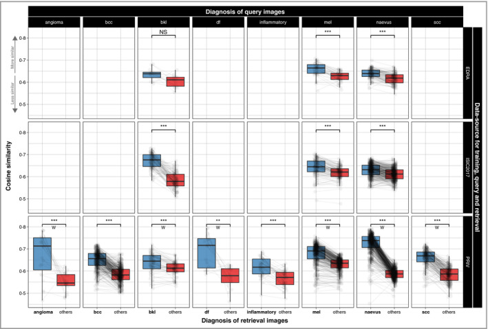
Measured visual similarity (cosine similarity) of images with the same diagnoses (blue) compared with others (red) in a dataset. Images of the same diagnoses are significantly rated higher in almost any subgroup, showing automated measurements of visual similarity can differentiate between diagnoses within a retrieval dataset. Lines are drawn between values for a single query image, and rows denote the dataset used for training, queries and image retrieval. Comparing differences was performed with a paired t‐test or a paired Wilcoxon signed rank test (W). ISIC2017, International Skin Imaging Collaboration, bcc, basal cell carcinoma; bkl, seborrhoeic keratoses; df, dermatofibromas; inflammatory, inflammatory lesions including dermatitis, lichen sclerosus, porokeratosis, rosacea, psoriasis, lupus erythematosus, bullous pemphigoid, lichen planus, granulomatous processes and artefacts mel, melanoma; scc, squamous cell carcinoma. NS, nonsignificant: P > 0·05, **P < 0·01, ***P < 0·001.
Using these ranked images for diagnostic predictions it was able to approximate a classic softmax‐based classifier with only few retrieval cases with regard to multiclass accuracy (Fig. 3 and Table 2). For the two datasets containing only three classes, CBIR outperformed the softmax‐based classification and had the highest accuracy when retrieving eight (EDRA, accuracy 0·762) and 16 similar cases (ISIC2017, accuracy 0·759), whereas in the PRIV dataset the best result with 32 retrievals (accuracy 0·629) was still below the corresponding softmax accuracy of 0·645. As can be seen in Figure 3, using more than 16 retrieved images did not consistently improve accuracy of CBIR.
Figure 3.
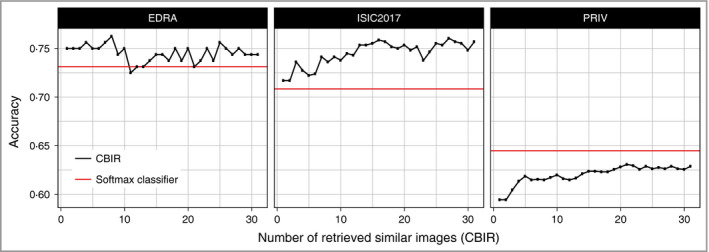
Frequency of correct specific diagnoses (accuracy) made within each dataset by either softmax‐based predictions (red) or content‐based image retrieval (CBIR) with a different number of retrieved similar images (black). Retrieval of a few images is already performing better in the three‐class datasets (EDRA, ISIC2017), whereas in the eight‐class (PRIV) dataset it takes over 20 images to approximate softmax‐based accuracy. ISIC2017, International Skin Imaging Collaboration.
Table 2.
Intra‐dataset performance metricsa
| Dataset, CBIR (k) | Accuracy | Sens@0·25 | Spec@0·25 | Sens@0·5 | Spec@0·5 | AUC | P‐value | P‐value (adj) |
|---|---|---|---|---|---|---|---|---|
| EDRA | ||||||||
| 2 | 0·75 | 72·7 (59·1–84·1) | 78·4 (70·7–85·3) | 72·7 (59·1–86·4) | 78·4 (70·7–85·3) | 0·782 (0·703–0·861) | 0·151 | b |
| 4 | 0·756 | 88·6 (79·5–97·7) | 64·7 (56–73·3) | 63·6 (50·0–77·3) | 86·2 (79·3–92·2) | 0·830 (0·760–0·900) | > 0·99 | b |
| 8 | 0·762 | 86·4 (75·0–95·5) | 70·7 (62·1–79·3) | 56·8 (40·9–70·5) | 89·7 (84·5–94·8) | 0·850 (0·784–0·916) | 0·342 | b |
| 16 | 0·744 | 84·1 (72·7–93·2) | 68·1 (59·5–76·7) | 52·3 (38·6–65·9) | 89·7 (83·6–94·8) | 0·842 (0·776–0·908) | 0·491 | b |
| 32 | 0·744 | 86·4 (75·0–95·5) | 69·8 (61·2–77·6) | 47·7 (31·8–61·4) | 92·2 (87·1–96·6) | 0·844 (0·776–0·912) | 0·499 | b |
| Softmax | 0·731 | 77·3 (65·9–88·6) | 75·9 (68·1–83·6) | 61·4 (47·7–75·0) | 84·5 (77·6–91·4) | 0·830 (0·759–0·901) | – | – |
| ISIC2017 | ||||||||
| 2 | 0·717 | 66·7 (58·1–75·2) | 83·2 (80–86·7) | 66·7 (58·1–75·2) | 83·2 (79·7–86·7) | 0·760 (0·713–0·807) | 0·006 | 0·073 |
| 4 | 0·727 | 76·1 (68·4–83·8) | 71·9 (67·5–76·0) | 53·8 (44·4–63·2) | 89·5 (86·5–92·4) | 0·785 (0·737–0·833) | 0·118 | b |
| 8 | 0·736 | 70·1 (61·5–78·6) | 78·4 (74·7–82·1) | 50·4 (41·9–59·8) | 90·4 (87·8–93·0) | 0·798 (0·751–0·845) | 0·431 | b |
| 16 | 0·759 | 70·9 (62·4–78·6) | 77·6 (73·9–81·3) | 50·4 (41–59·8) | 92·8 (90·4–95·2) | 0·806 (0·759–0·853) | 0·785 | b |
| 32 | 0·753 | 68·4 (59·8–76·9) | 77·3 (73·6–81·0) | 41·0 (32·5–49·6) | 94·3 (92·2–96·3) | 0·799 (0·751–0·846) | 0·354 | b |
| Softmax | 0·708 | 70·9 (62·4–79·5) | 74·9 (70·8–78·6) | 60·7 (52·1–69·2) | 86·7 (83·4–89·5) | 0·810 (0·765–0·854) | – | – |
| PRIV | ||||||||
| 2 | 0·594 | 82·7 (80·2–85·1) | 66·8 (63·1–70·6) | 82·7 (80·2–85·3) | 67·0 (63·1–70·6) | 0·791 (0·770–0·813) | < 0·001 | < 0·001 |
| 4 | 0·614 | 89·3 (87·2–91·3) | 54·4 (50·5–58·3) | 79·4 (76·8–81·9) | 73·9 (70·3–77·3) | 0·822 (0·802–0·843) | 0·002 | 0·032 |
| 8 | 0·615 | 87·9 (85·9–89·9) | 60·6 (56·9–64·4) | 74·7 (72–77·4) | 77·9 (74·8–81·2) | 0·843 (0·823–0·862) | 0·597 | b |
| 16 | 0·624 | 87·4 (85·2–89·5) | 63·9 (60–67·8) | 74·2 (71·2–76·9) | 81·2 (78·1–84·3) | 0·852 (0·833–0·871) | 0·456 | b |
| 32 | 0·629 | 87·2 (84·9–89·3) | 66·2 (62·4–69·8) | 73·2 (70·5–75·9) | 82·2 (78·9–85·1) | 0·859 (0·840–0·878) | 0·072 | b |
| Softmax | 0·645 | 87·7 (85·5–89·7) | 62·6 (58·7–66·3) | 75·3 (72·5–78·0) | 79·7 (76·6–82·7) | 0·847 (0·827–0·867) | – | – |
CBIR, content‐based image retrieval.
aArea under the receiver operating characteristic curve (AUC) is calculated for detecting any malignant skin tumour in the corresponding dataset. Numbers in parentheses represent 95% confidence intervals. Sensitivity (Sens) and specificity (Spec) are calculated at 25% and 50% retrieved malignant cases (CBIR) or predicted probability of malignancy (softmax). P‐values, provided as original and as P‐value (adj) with correction for multiple testing by the method of Holm,27 denote difference of CBIR‐based AUC values from softmax‐based ones. bSignifies nonevaluated comparisons after correction for multiple testing. The best result within each dataset and metric is shown in bold.
In all three datasets, showing only two retrieved images resulted in decreased performance in detecting skin cancer as measured by the AUC, where the difference was significant for the eight‐class dataset (EDRA 0·782 vs. 0·830, P = 1·0; ISIC2017 0·760 vs. 0·810, P = 0·073; PRIV 0·791 vs. 0·847, P < 0·001).
Figure 4 shows the ROC curve of the EDRA intra‐dataset evaluation when fixing the CBIR output to 16 images, where disregarding a small frequency of malignant cases in the images did not change sensitivity substantially. Fixing the outputs to 16 cases, and labelling a query case ‘malignant’ if at least 25% of retrievals showed a malignant lesion, resulted in a sensitivity of 84·1% and a specificity of 68·1% in the EDRA dataset, 70·9% and 77·6% in the ISIC2017 and 87·4% and 63·9% in the PRIV dataset, respectively (Table 2).
Figure 4.

Receiver operating characteristic curve for detecting melanoma when retrieving 16 similar images with content‐based image retrieval (CBIR) (grey), showing different thresholds of needed malignant retrieval images (‘predict melanoma when x of 16 retrieved images are melanomas’), in addition to softmax‐based probabilities (red). Network training‐, query‐ and retrieval‐images are from EDRA. AUC, area under the receiver operating characteristic curve.
New‐source classification
Figure 5 and Table 3 show mean average precision values of networks trained and tested on different datasets, with different CBIR resource databases used. In other words, the images to be diagnosed, the images a CNN retrieves similar cases from and the images the CNN was trained on can all originate from different sources. Softmax‐based predictions from three‐class‐trained networks (EDRA and ISIC2017) perform worse on predicting the eight‐class dataset (PRIV) with mAP values of 0·184 and 0·198, respectively. Using the target source as a CBIR resource improved mAP to up to 0·368 and 0·403, respectively. This is because previously ‘unknown’ classes can still be retrieved as those networks transfer the ability to distinguish diagnoses through visual similarity (see Fig. 6). The best CBIR performance is obtained with combinations where training, testing and resource are from the same source.
Figure 5.

Mean average precision (mAP) of a ResNet‐50 network trained on EDRA dataset images. Predictions were made either through softmax probabilities (red line) or class‐frequencies of content‐based image retrieval (CBIR) (black). Softmax predictions perform worst on predicting PRIV dataset images, as the networks are not able to predict five of the eight classes in any case (first two columns, bottom row). CBIR retrieving from EDRA and ISIC2017 suffers from the same shortcomings, but was able to predict better when using PRIV‐source retrieval images (bottom right). In general, CBIR performs best when using retrieval images from the same source as the test images (descending diagonal), and here performed better on new data than softmax predictions. Re‐training the network on those new‐source images (blue) in turn outperformed CBIR again. ISIC2017, International Skin Imaging Collaboration.
Table 3.
Mean average precision between datasetsa
| TRAIN | TEST | CBIR | CBIR 2 | CBIR 4 | CBIR 8 | CBIR 16 | CBIR 32 | Softmax |
|---|---|---|---|---|---|---|---|---|
| EDRA | 0·632 | 0·681 | 0·702 | 0·748 | 0·775 | |||
| EDRA | ISIC2017 | 0·466 | 0·507 | 0·579 | 0·638 | 0·662 | 0·761 | |
| PRIV | 0·405 | 0·490 | 0·520 | 0·563 | 0·573 | |||
| EDRA | 0·385 | 0·417 | 0·429 | 0·444 | 0·444 | |||
| EDRA | ISIC2017 | ISIC2017 | 0·465 | 0·513 | 0·576 | 0·585 | 0·582 | 0·456 |
| PRIV | 0·388 | 0·398 | 0·425 | 0·438 | 0·445 | |||
| EDRA | 0·154 | 0·161 | 0·165 | 0·172 | 0·177 | |||
| PRIV | ISIC2017 | 0·150 | 0·163 | 0·170 | 0·179 | 0·188 | 0·184 | |
| PRIV | 0·249 | 0·284 | 0·310 | 0·338 | 0·368 | |||
| EDRA | 0·524 | 0·591 | 0·583 | 0·624 | 0·604 | |||
| EDRA | ISIC2017 | 0·410 | 0·448 | 0·487 | 0·488 | 0·512 | 0·524 | |
| PRIV | 0·374 | 0·416 | 0·441 | 0·453 | 0·459 | |||
| EDRA | 0·376 | 0·403 | 0·459 | 0·504 | 0·537 | |||
| ISIC2017 | ISIC2017 | ISIC2017 | 0·583 | 0·654 | 0·697 | 0·725 | 0·734 | 0·745 |
| PRIV | 0·405 | 0·423 | 0·439 | 0·468 | 0·483 | |||
| EDRA | 0·149 | 0·158 | 0·167 | 0·175 | 0·182 | |||
| PRIV | ISIC2017 | 0·159 | 0·172 | 0·183 | 0·191 | 0·200 | 0·198 | |
| PRIV | 0·269 | 0·316 | 0·377 | 0·389 | 0·403 | |||
| EDRA | 0·514 | 0·597 | 0·637 | 0·647 | 0·640 | |||
| EDRA | ISIC2017 | 0·434 | 0·465 | 0·498 | 0·540 | 0·566 | 0·641 | |
| PRIV | 0·543 | 0·552 | 0·582 | 0·597 | 0·629 | |||
| EDRA | 0·371 | 0·403 | 0·434 | 0·458 | 0·475 | |||
| PRIV | ISIC2017 | ISIC2017 | 0·543 | 0·596 | 0·649 | 0·667 | 0·688 | 0·551 |
| PRIV | 0·419 | 0·446 | 0·468 | 0·498 | 0·528 | |||
| EDRA | 0·152 | 0·161 | 0·167 | 0·171 | 0·177 | |||
| PRIV | ISIC2017 | 0·158 | 0·169 | 0·181 | 0·188 | 0·197 | 0·598 | |
| PRIV | 0·405 | 0·472 | 0·517 | 0·545 | 0·568 |
aTRAIN denotes dataset the ResNet‐50 architecture was trained on, TEST the origin of test images, and content‐based image retrieval (CBIR) origin of retrieval images. While CBIR was able to approximate softmax‐based predictions between the three‐class datasets (EDRA and ISIC2017) when using same‐source TEST and CBIR sets, it outperformed three‐class trained networks on the eight‐class PRIV dataset as it is able to recognize unseen classes through the larger resource dataset. ISIC2017, International Skin Imaging Collaboration.
Figure 6.

Mean cosine similarities of PRIV retrieval images with the same (blue) or different (red) diagnosis for the corresponding PRIV query images. Cosine similarity is calculated by feature extraction via ResNet‐50 networks trained for classification on different training datasets (rows). Compared with the PRIV‐trained network, those trained on different sources (row EDRA and ISIC2017) transfer their ability to distinguish specific diagnoses through visual similarity except for seborrhoeic keratoses (bkl) cases. Lines are drawn between values for the same query image. W, paired Wilcoxon signed‐rank test was used instead of paired t‐test; ISIC2017, International Skin Imaging Collaboration; bcc, basal cell carcinoma; df, dermatofibromas; mel, melanoma; scc, squamous cell carcinoma. NS, nonsignificant: P > 0·05, **P < 0·01, ***P < 0·001; grey indicators denote nonadjusted P‐values as these comparisons were omitted during correction for multiple testing (see statistics section).
Discussion
Current CNN classifiers perform well but commonly behave as black boxes during inference and preclude meaningful integration of their findings to a clinical‐decision process. Having an intuitive, ‘explainable’, output of an automated classifier that complements – rather than overrides – a clinical‐decision process may be more desirable and can enhance efficient use of the time of healthcare workers. Compared with other techniques for explainable artificial intelligence28 such as image captioning and visual question answering,12 we hypothesize that showing similar cases with their ground truth may be even more intuitive. Similar images found by CBIR further comprehensibly reveal the knowledge base of a network decision and may conceive when not to trust the automated system. More specifically, if users notice retrieved cases look nothing like the query image, they could intuitively decide the CNN cannot help in that case. Herein we show that CBIR can perform on a par with softmax‐based predictions of a ResNet‐50 network on accuracy of skin cancer detection, in addition to multiclass accuracy and mean average precision (Table 2).
We describe reasonably good metrics for formal evaluation of a CBIR system, but more current architectures may be able to reach even higher accuracy. We hypothesize that, with increasing accuracy of a network, accuracy of CBIR will rise accordingly. The true advantage of CBIR may lie in the fact that a human reader can select the most fitting and relevant examples from the provided image‐subset and is not restricted to the strict counting and weighting used for calculations in this manuscript. We suspect having such a ‘human‐in‐the‐loop’ would give a much higher diagnostic precision in practice, which should be subject to future studies.
Deep learning literature dealing with image classification commonly presents accuracy metrics measured on the same dataset‐source incorporating the same diagnostic classes. Relying on those experimental results when implementing an automated classifier in clinical practice may be precarious, as an end‐user may take images with a different camera, on patients with different skin types, with different class distributions – and even with disease classes the network has not encountered before. For these reasons a classifier with a fixed set of diagnoses may fail in unexpected ways that would go unnoticed if the output is merely a probability of specific diagnoses. Neural networks trained for classification by design are limited to predict classes they have seen during the training period. Currently, to our knowledge, no available dataset comes close to encompassing all clinically possible classes. Further, class definitions of medical entities may change over time with new biological insights. The CBIR method described herein shows that classifiers knowing only three classes are able to generalize better to a new dataset with eight classes than their softmax‐based predictions (Table 3). The highest accuracy can still be obtained through fine‐tuning a network on the target data source (blue lines in Fig. 5), but such a re‐training period may not be feasible when retrieval data‐sources are not accessible for training because of data protection regulations or lack of machine learning resources.
In contrast to decision support systems with a fixed performance and cut‐off that needs to undergo clinical testing,29 CBIR as a dynamic and potentially vendor‐independent, decision support system may be easier to expand and update in practice with growing search datasets and improved models.
There are some limitations to our study. As the results from a previous study by Kawahara et al.16 were not public until the end of our experiments we did not perform a sample size calculation, so this work needs to be regarded as an exploratory pilot study. We trained the ResNet‐50 architecture on the datasets with reasonable effort on fine‐tuning, data augmentation and hyperparameter tuning, but did not pursue maximum classification accuracy. Therefore, achievable values may be higher as shown by Han et al.,4 but we expect a better classifier using a larger image dataset to improve CBIR in a similar way. All data herein is suffering from selection bias (images were found worthwhile to be photographed by a physician) and verification bias. A user‐focused and prospective analysis of such a decision support will be able to give more insight into clinical applicability. Document retrieval studies usually use a different set of metrics where mean average precision is defined differently. We chose the used metrics and definitions to reflect clinically meaningful outcomes rather than retrieval performance.
In conclusion, in this work we show that automated retrieval of few visually similar dermatoscopic images approximate accuracy of softmax‐based prediction probabilities. Further, CBIR may improve performance of trained networks in new sets and unseen classes when there is no possibility of fine‐tuning of a network on new data.
Supporting information
File S1 Training implementation details and mean average precision definitions.
Powerpoint S1 Journal Club Slide Set.
Video S1. Author video.
Funding sources MetaOptima Technology Inc.
Conflicts of interest MetaOptima Technology Inc., where M.R. holds the position of Chief Technology Officer, provided access to deep learning hardware, employs J.Y. and provided an unrestricted research grant to P.T. for conducting a 1‐year post‐doc fellowship at Simon Fraser University. G.A. serves as a medical advisor to MetaOptima Technology Inc. MetaOptima Technology offers a content‐based image retrieval (CBIR)‐based educational tool to clinicians called Visual Search that was not part of the presented experiments.
Plain language summary available online
References
- 1. Menzies S, Bischof L, Talbot H et al The performance of solarscan: an automated dermoscopy image analysis instrument for the diagnosis of primary melanoma. Arch Dermatol 2005; 141:1388–96. [DOI] [PubMed] [Google Scholar]
- 2. Dreiseitl S, Binder M, Vinterbo S, Kittler H. Applying a decision support system in clinical practice: results from melanoma diagnosis. AMIA Annu Symp Proc 2007; 2007:191–5. [PMC free article] [PubMed] [Google Scholar]
- 3. Esteva A, Kuprel B, Novoa RA et al Dermatologist‐level classification of skin cancer with deep neural networks. Nature 2017; 542:115–18. [DOI] [PMC free article] [PubMed] [Google Scholar]
- 4. Han SS, Kim MS, Lim W et al Classification of the clinical images for benign and malignant cutaneous tumors using a deep learning algorithm. J Invest Dermat 2018; 138:1529–38. [DOI] [PubMed] [Google Scholar]
- 5. Haenssle HA, Fink C, Schneiderbauer R et al Man against machine: diagnostic performance of a deep learning convolutional neural network for dermoscopic melanoma recognition in comparison to 58 dermatologists. Ann Oncol 2018; 29:1836–42. [DOI] [PubMed] [Google Scholar]
- 6. Gulshan V, Peng L, Coram M et al Development and Validation of a deep learning algorithm for detection of diabetic retinopathy in retinal fundus photographs. JAMA 2016; 316:2402–10. [DOI] [PubMed] [Google Scholar]
- 7. Rajpurkar P, Irvin J, Zhu K et al CheXNet: radiologist‐level pneumonia detection on chest x‐rays with deep learning. Available at: http://arxiv.org/abs/1711.05225 (last accessed 5 October 2018).
- 8. Codella NCF, Gutman D, Celebi ME et al Skin lesion analysis toward melanoma detection: a challenge at the 2017 International Symposium on Biomedical Imaging (ISBI), Hosted by the International Skin Imaging Collaboration (ISIC). Available at: http://arxiv.org/abs/1710.05006 (last accessed 5 October 2018).
- 9. Tschandl P, Rosendahl C, Kittler H. The HAM10000 dataset: a large collection of multi‐source dermatoscopic images of common pigmented skin lesions. Sci Data 2018; 5:180161. [DOI] [PMC free article] [PubMed] [Google Scholar]
- 10. Finlayson SG, Chung HW, Kohane IS, Beam AL. Adversarial attacks against medical deep learning systems. Available at: http://arxiv.org/abs/1804.05296 (last accessed 15 September 2018).
- 11. Girardi D, Küng J, Kleiser R et al Interactive knowledge discovery with the doctor‐in‐the‐loop: a practical example of cerebral aneurysms research. Brain Inform 2016; 3:133–43. [DOI] [PMC free article] [PubMed] [Google Scholar]
- 12. Park DH, Hendricks LA, Akata Z et al Attentive explanations: justifying decisions and pointing to the evidence. Available at: http://arxiv.org/abs/1612.04757 (last accessed 5 October 2018).
- 13. Piplani T, Bamman D. DeepSeek: Content based image search & retrieval. Available at: http://arxiv.org/abs/1801.03406 (last accessed 5 October 2018).
- 14. Parkhi OM, Vedaldi A, Zisserman A. Deep face recognition In: Proceedings of the British Machine Vision Conference (BMVC) (Xianghua Xie MWJ, Tam GKL, eds). London: BMVA Press, 2015; 41.1–41.12. [Google Scholar]
- 15. Shi X, Sapkota M, Xing F et al Pairwise based deep ranking hashing for histopathology image classification and retrieval. Pattern Recognit 2018; 81:14–22. [Google Scholar]
- 16. Kawahara J, Daneshvar S, Argenziano G, Hamarneh G. 7‐Point checklist and skin lesion classification using multi‐task multi‐modal neural nets. IEEE J Biomed Health Inform 2018; 10.1109/JBHI.2018.2824327. [DOI] [PubMed] [Google Scholar]
- 17. Argenziano G, Soyer P, De Giorgi V et al Interactive Atlas of Dermoscopy. Dermoscopy: a tutorial (Book) and CD‐ROM. Milan: Edra Medical Publishing and New Media, 2000. [Google Scholar]
- 18. He K, Zhang X, Ren S, Sun J. Deep residual learning for image recognition. Available at: https://www.cv-foundation.org/openaccess/content_cvpr_2016/papers/He_Deep_Residual_Learning_CVPR_2016_paper.pdf (last accessed 5 October 2018).
- 19. Russakovsky O, Deng J, Su H et al ImageNet Large scale visual recognition challenge. Int J Comput Vis 2015; 115:211–52. [Google Scholar]
- 20. Pedregosa F, Varoquaux G, Gramfort A et al Scikit‐learn: machine learning in Python. J Mach Learn Res 2011; 12:2825–30. [Google Scholar]
- 21. Paszke A, Gross S, Chintala S et al Automatic differentiation in PyTorch. Presented at the 31st Conference on Neural Information Processing Systems (NIPS 2017), Long Beach, CA, U.S.A., 4–9 December 2017. [Google Scholar]
- 22. Hunter JD. Matplotlib: A 2D graphics environment. Comput Sci Eng 2007; 9:90–5. [Google Scholar]
- 23. R Core Team . R: A Language and Environment for Statistical Computing. Vienna, Austria; 2017. Available from: https://www.R-project.org/ (last accessed 5 October 2018).
- 24. Wickham H. ggplot2: Elegant Graphics for Data Analysis. New York: Springer‐Verlag, 2016. Available from: http://ggplot2.org (last accessed 5 October 2018). [Google Scholar]
- 25. Robin X, Turck N, Hainard A et al pROC: an open‐source package for R and S+ to analyze and compare ROC curves. BMC Bioinformatics 2011; 12:77. [DOI] [PMC free article] [PubMed] [Google Scholar]
- 26. DeLong ER, DeLong DM, Clarke‐Pearson DL. Comparing the areas under two or more correlated receiver operating characteristic curves: a nonparametric approach. Biometrics 1988; 44:837–45. [PubMed] [Google Scholar]
- 27. Holm S. A Simple sequentially rejective multiple test procedure. Scand J Statist 1979; 6:65–70. [Google Scholar]
- 28. Holzinger A, Biemann C, Pattichis CS, Kell DB. What do we need to build explainable AI systems for the medical domain? Available at: http://arxiv.org/abs/1712.09923 (last accessed 5 October 2018).
- 29. Monheit G, Cognetta AB, Ferris L et al The performance of MelaFind: a prospective multicenter study. Arch Dermatol 2011; 147:188–94. [DOI] [PubMed] [Google Scholar]
Associated Data
This section collects any data citations, data availability statements, or supplementary materials included in this article.
Supplementary Materials
File S1 Training implementation details and mean average precision definitions.
Powerpoint S1 Journal Club Slide Set.
Video S1. Author video.