The Joinpoint-Jump and Joinpoint-Comparability Ratio Model for Trend Analysis with Applications to Coding Changes in Health Statistics

Abstract

Analysis of trends in health data collected over time can be affected by instantaneous changes in coding that cause sudden increases/decreases, or “jumps,” in data. Despite these sudden changes, the underlying continuous trends can present valuable information related to the changing risk profile of the population, the introduction of screening, new diagnostic technologies, or other causes. The joinpoint model is a well-established methodology for modeling trends over time using connected linear segments, usually on a logarithmic scale. Joinpoint models that ignore data jumps due to coding changes may produce biased estimates of trends. In this article, we introduce methods to incorporate a sudden discontinuous jump in an otherwise continuous joinpoint model. The size of the jump is either estimated directly (the Joinpoint-Jump model) or estimated using supplementary data (the Joinpoint-Comparability Ratio model). Examples using ICD-9/ICD-10 cause of death coding changes, and coding changes in the staging of cancer illustrate the use of these models.

1. Introduction

“Is the trend changing?” This question underlies trend analysis in the field of disease prevention, control and surveillance. Data describing disease incidence, mortality and other health series are reported over time. Data items in those series are often recorded or classified based on certain types of coding systems, and sudden changes in code structure or coding rules over time are not uncommon. For example, in 1999, the Tenth Revision of the International Classification of Diseases (ICD-10) replaced the Ninth Revision (ICD-9) for coding causes of death used for mortality statistics (Anderson et al. 2001). In another example, cancer staging algorithms change across time periods (Amin 2017). Newer staging system are added by cancer registries to keep definitions consistent with the current understanding of diseases. Such coding changes may cause discontinuous increases/decreases, or “jumps,” in the data series, even though it may not affect the underlying trend.

In the past, the Joinpoint model, developed by the National Cancer Institute, has been widely used to characterize and report trends in health statistics and other time data series (Kim et al. 2000; Clegg et al. 2009). The model has log linear segments and has distinct advantages over other models, such as the polynomial fitted model, and is easier to interpret (Clegg et al. 2009). However, when there is a discontinuity or jump that occurs in the data, the Joinpoint model could potentially result in a misleading interpretation of trend changes, as the jump could be the result of a one-time external circumstance, which may not be interpreted as a changing point in the data.

In some cases the size of the jump is known or can be estimated. In the case of ICD code changes, a comparison of causes of death coded to both ICD-9 and ICD-10 was conducted. The National Center for Health Statistics (NCHS) of the Centers for Disease Control and Prevention (CDC) double coded 1996 death certificates using both the ICD-9 and ICD-10 algorithms and published “comparability ratios” and their standard errors (National Center for Health Statistics 2009). The comparability ratios estimate the size of the jump in mortality rates associated with the coding change. In this case, we propose a Joinpoint-Comparability Ratio (JP-CR) method to accommodate the jumps, that is, converting the data before the jump by the size of the jump and then applying the Joinpoint model to the converted data. The standard error of the converted data can be adjusted by combining the standard error of the CR and the standard error associated with the original data. This approach may work well if the goal is to capture the trend of the time series data given that the jump size is known or has been estimated based on an external study.

However, the requirement of knowing the jump size makes the analysis more difficult because the size of the jump needs to be estimated, and in many cases, this may not be feasible. Motivated by the need for trend analysis with a sudden jump where the size of the jump is unknown, we propose another method called Joinpoint-Jump (JP-Jump) model. The model minimizes the effect of the jumps on trend analysis. Unlike the JP-CR method, the JP-Jump model simultaneously estimates the size of the jump, as well as the changes in trend.

The remainder of this article is organized as follows. Section 2 briefly reviews the Joinpoint model and presents the JP-CR and JP-Jump models. In Section 3, we consider several applications. In one application, the proposed models are applied to US mortality data where there is a coding change from ICD-9 to ICD-10 starting in 1999. In another application, we apply the proposed models to cancer incidence data to test the difference between two cancer staging systems. Section 4 discusses practical considerations in choosing between the two models.

2. The Joinpoint, Joinpoint-Jump (JP-Jump) and Joinpoint-Comparability Ratio (JP-CR) Models

2.1. The Joinpoint Model (JP) – A Brief Review

The Joinpoint model is a segmented linear regression model. Suppose that we observe (x₁, γ₁), … ,(x_n, γ_n), γ_i is an age-adjusted cancer incidence/mortality rate at time x_i and y_i = log(γ_i). The Joinpoint model, propsed by Kim et al. (2000), assumes

$$\begin{gathered} y_i=\mathit{\text{log}}\left({\gamma }_i\right)={\alpha }_1+{\beta }_1{x}_i+{\delta }_1{\left(x_i-{\tau }_1\right)}^{+}+\dots +{\delta }_{\kappa }{\left(x_i-{\tau }_{\kappa }\right)}^{+}+{ϵ}_i, \\ i=1,\dots ,n, \end{gathered}$$ (1)

where ϵ_i are independent errors, the notation a⁺ = a if a > 0, and a⁺ = 0 otherwise. In this model, the mean function of y_i is linear segments connected at change-points τ₁ < ⋯ < τ_κ. The locations of change-points τ_i as well as the number of change-points k are assumed to be unknown and need to be estimated from the data. Assuming the number of change-points is given, say κ = K, the locations of K joinpoints, τ₁, … , τ_K, are estimated by the grid search method described by Lerman (1980) or a continuous fitting method proposed by Hudson (1966). The overall least squares estimates of the regression coefficients are then obtained based on the estimated joinpoints. Once the least squares fit is obtained for a model with κ = K, an iterative procedure is used to determine whether addition of joinpoints significantly reduces the residual sum of squares. The procedure iteratively tests the null hypothesis that there are K₀ joinpoints against the alternative hypothesis that there are K₁ joinpoints where K₁ > K₀, and usually begins with K₀ and K₁ respectively being the pre-specified minimum and maximum number of joinpoints allowed. Due to the fact that classical asymptotic theory does not work in this situation, a Monte Carlo permutation test is used to determine the p-value of the test. First permute the residuals from fitting the model under the null hypothesis. For each permutation, add the permutated residuals back to the fitted values and refit the permutated data under the alternative hypothesis, and obtain the F-statistics as a goodness-of-fit measure. The p-value of the test is then calculated from the distribution of the goodness-of-fit statistics. If the null hypothesis is rejected, then test H₀: κ = K₀ + 1 versus H₁: κ = K₁; otherwise, test H₀: κ = K₀ versus H₁: κ = K₁ − 1. Tests are repeatedly conducted until for some K, the testing of H₀: κ = K versus H₁: κ = K + 1 is performed. Because the procedure is based on multiple testing, the significance level of each test is adjusted to maintain the overall level under α, which is the probability of over-fitting the model. Instead of permutation test, model selection methods based on the Bayes Information Criterion (BIC) or a modified BIC, can work as faster alternatives.

2.2. The JP-Jump Model

We consider a model where a jump occurs at a known location s, and we allow s to be a possible change-point. Denote the observed rate at the time x_i as γ_i, i = 1, … , n. The jump location is incorporated into a joinpoint model by assuming

$$y_i=\mathit{\text{log}}\left({\gamma }_i\right)={\alpha }_1+{\beta }_1{x}_i+{\delta }_1{\left(x_i-{\tau }_1\right)}^{+}+\cdots +{\delta }_{\kappa }{\left(x_i-{\tau }_{\kappa }\right)}^{+}+\lambda \text{I}\left(x_i\ge s\right)+{ϵ}_i,$$ (2)

where τ₁ < … < τ_κ are unknown change-points, s is a known location of a jump, λ represents the jump size, ϵ_i are independent errors N(0, σ²), and I(A) = 1 if A is true and 0 otherwise. If j denotes the index value such that τ_j < s < τ_j+1, this model can also be expressed as

$$E\left(y_i\mid x_i\right)=\{\begin{array}{cc}{\alpha }_1+{\beta }_1{x}_i& \mathit{\text{ if }}{\tau }_0\le x_i\le {\tau }_1\\ ⋮& ⋮\\ {\alpha }_j+{\beta }_j{x}_i& \mathit{\text{ if }}{\tau }_{j-1}<x_i\le {\tau }_j\\ {\alpha }_{j+1}+{\beta }_{j+1}{x}_i& \mathit{\text{ if }}{\tau }_j<x_i<s\\ {\alpha }_{j+1}+\lambda +{\beta }_{j+1}{x}_i& \mathit{\text{ if }}s\le x_i\le {\tau }_{j+1}\\ {\alpha }_{j+2}+\lambda +{\beta }_{j+2}{x}_i& \mathit{\text{ if }}{\tau }_{j+1}<x_i\le {\tau }_{j+2}\\ ⋮& ⋮\\ {\alpha }_{\kappa +1}+\lambda +{\beta }_{k+1}{x}_i& \mathit{\text{ if }}{\tau }_{\kappa }<x_i\le {\tau }_{\kappa +1}\end{array},$$ (3)

where τ₀ = min{x_i}, τ_κ+1 = max{x_i}, and α_m + β_mτ_m = α_m+1 + β_{m + 1} τ_m for m = 1, …, κ. Equations (2) and (3) are equivalent when

$${\alpha }_l={\alpha }_1-\sum _{u=1}^{l-1}{\delta }_u{\tau }_u,l=2,\dots ,\kappa +1,$$

$${\beta }_l={\beta }_1+\sum _{u=1}^{l-1}{\delta }_u,l=2,\dots ,\kappa +1.$$

To fit the model, at any possible locations of joinpoints (τ₁, … , τ_κ) = (t₁, … , t_κ) = t′, we obtain the least squares estimate of θ = (α₁, β₁, δ₁, … , δ_κ, λ)′as

$$\widehat{\theta }(t)={\left(X_t^{\prime }{X}_t\right)}^{-1}{X}_t^{\prime }y,$$

where y₁ = (y₁, … ,y_n)′, and

$$X_t=\left(\begin{array}{cccccc}1& x_1& {\left(x_1-t_1\right)}^{+}& \cdots & {\left(x_1-t_{\kappa }\right)}^{+}& 0\\ ⋮& ⋮& ⋮& ⋮& ⋮& ⋮\\ 1& x_j& {\left(x_j-t_1\right)}^{+}& \cdots & {\left(x_j-t_{\kappa }\right)}^{+}& 0\\ 1& x_{j+1}& {\left(x_{j+1}-t_1\right)}^{+}& \cdots & {\left(x_{j+1}-t_{\kappa }\right)}^{+}& 1\\ ⋮& ⋮& ⋮& ⋮& ⋮& ⋮\\ 1& x_n& {\left(x_n-t_1\right)}^{+}& \cdots & {\left(x_n-t_{\kappa }\right)}^{+}& 1\end{array}\right).$$

The number of change-points κ can be determined by a Monte Carlo permutation test and the locations of change-points τ_i are obtained by a grid search method. A grid search finds the estimate of τ = (τ₁, … , τ_κ)′, denoted by $\widehat{\tau }$, by minimizing the residual sum of squares RSS(t) over all possible choices of t. Given $\widehat{\tau }$, the overall least squares estimate is calculated, denoted by $\widehat{\theta }\left(\widehat{\tau }\right)$. After fitting the model and calculating the residual sum of squares for the fitted model, the number of change-points can be either selected by using a permutation procedure or BIC method.

Instead of calculating the constrained standard error of $\widehat{\theta }$, the standard error is calculated by unconstrained standard error estimate. For all the segments except the one that includes the known change-point s, the standard error is calculated as in the regular Joinpoint model. For the segment where s lies, say [x_j1, … , x_jm], E(y|x) = α_j+1 + β_j+1x + λI(x ≥ s) for x ∈ [x_j1, … , x_jm], the standard error estimates of $\left({\widehat{\alpha }}_{j+1},{\widehat{\beta }}_{j+1},\widehat{\lambda }\right)$, can be calculated by using

$${\left[SE\left({\widehat{\alpha }}_{j+1},{\widehat{\beta }}_{j+1},\widehat{\lambda }\right)\right]}^2={\widehat{\sigma }}^2{\left(X_{\left[x_{j1},x_{jm}\right]}^{\prime }{X}_{\left[x_{j1},x_{jm}\right]}\right)}^{-1},$$

where

$$X_{\left[x_{j1},x_{jm}\right]}=\left(\begin{array}{ccc}1& x_{j1}& 0\\ ⋮& ⋮& ⋮\\ 1& x_j& 0\\ 1& x_{j+1}& 1\\ ⋮& ⋮& ⋮\\ 1& x_{jm}& 1\end{array}\right).$$

Like the regular Joinpoint model, this unconstrained standard error estimate tends to perform better than the constrained standard error estimate, see Kim et al. (2008).

In the JP-Jump model, λ, representing the size of the jump, is estimated simultaneously with other parameters α₁, … , α_κ+1 and β₁, … , β_κ+1. The variance of $\widehat{\lambda }$ can be obtained as well. To compare the rates after and before the jump, we consider the ratio of the after-jump rate and the before-jump rate. We call it the model-based comparability ratio, which can be estimated directly from the JP-Jump model. Specifically, let ρ denote the model-based comparability ratio, calculated as

$$\rho =\frac{\text{exp}\left(E\left(y\mid x=s^{+}\right)\right)}{\text{exp}\left(E\left(y\mid x=s^{-}\right)\right)}=\frac{\text{exp}\left({\alpha }_{j+1}+{\beta }_{j+1}x+\lambda \right)}{\text{exp}\left({\alpha }_{j+1}+{\beta }_{j+1}x\right)}=e^{\lambda },$$ (4)

where x = s⁺ and x = s⁻denote the right and left side limits of x at s. The model-based comparability ratio ρ is estimated by $\widehat{\rho }=\text{exp}(\widehat{\lambda })$, and the standard error of $\widehat{\rho }$ can be estimated by using the delta method, which is

$$\mathit{\text{Var}}(\widehat{\rho })\approx {\left(e^{\widehat{\lambda }}\right)}^2\mathit{\text{Var}}(\widehat{\lambda }),$$

and $SE(\widehat{\rho })=e^{\widehat{\lambda }}SE(\widehat{\lambda })$. For any α ∈ (0, 1), the (1 – α) × 100% approximate confidence interval for ρ can be constructed by $\left[\widehat{\rho }-z_{\alpha /2}SE(\widehat{\rho }),\widehat{\rho }+z_{\alpha /2}SE(\widehat{\rho })\right]$, where z_α/2 denotes the upper α/2-th percentile of the standard normal distribution.

2.3. The Joinpoint-Comparability Ratio Model (JP-CR)

For this method, we assume that the analyst is provided with a comparability ratio and its variance from an external source. The ratio, denoted by C, represents a ratio of the case counts after the change to before the change. If C is 1, the total net count is not affected by the code change, even if individual records may be impacted. If C is less than 1, fewer events are classified to this cause under the new coding system compared to the previous system.

Conversely, if the ratio is greater than 1, more events are classified to this cause under the new coding system than under the previous one.

Recall that the incidence/mortality rate is denoted by γ. The comparability ratio method specifically uses the following steps:

• Step 1. For data before the coding change, find the Comparability ratio-Modified rate, γ^CM, by multiplying the original rate by the comparability ratio, that is,

  $${\gamma }^{CM}=\gamma \times C.$$

• Step 2. Combine the adjusted data before the coding change and the original data after the coding change. Analyze the trend by applying the regular Joinpoint model to the combined data.

• Step 3. Before graphing the results, convert the fitted rates prior to the coding change derived from Step 2 (denoted by ${\widehat{\gamma }}^{CM}$), back to the original scale by dividing by the comparability ratio, $\widehat{\gamma }=\frac{{\widehat{\gamma }}^{CM}}{C}$.

3. Results

3.1. US Mortality With Code Changes From ICD-9 To ICD-10

The International Classification of Diseases is revised periodically to stay current of medical knowledge and advances (Anderson et al. 2001). The most recent code changes occurred between 1998 and 1999 when ICD-10 replaced ICD-9. The coding changes have impacts on some of the major causes of death in the United States. Comparability ratios developed by Anderson et al. (2001) are designed to quantify the impact of the coding change. Although the first year with new code is 1999, the comparability ratios presented by Anderson et al. are based on double-coding the same deaths occurring in 1996 by both ICD-9 and ICD-10. For each cause of death, the comparability ratio, denoted by C, is calculated as

$$C=\frac{D_{ICD-10}}{D_{ICD-9}},$$

where D_ICD-10 and D_ICD-9 are the number of deaths classified by ICD-10 and ICD-9 respectively. We demonstrate these coding changes using two examples, one with a large comparability ratio (septicemia) and one with relatively small comparability ratio (melanoma).

3.1.1. Septicemia Mortality With Code Changes From ICD-9 To ICD-10

The published comparability ratio for septicemia is 1.1949 (Anderson et al. 2001), which represents nearly 20% more deaths according to the ICD-10 coding paradigm than that of ICD-9. Under ICD-10, septicemia is selected as the underlying cause of death over pneumonia when both are listed on the death certificate; septic shock, coded in ICD-9 in a different category is coded as “Unspecified septicemia” in ICD-10. The mortality rates due to septicemia from 1979 to 2010 for all races and both sexes along with the fitted trends based on the regular Joinpoint model (called JP-Standard model hereafter) are shown in Figure 1. The JP-Standard model does not take into account the code change information and the fitted line indicates there is a large upward trend from 1996 to 2000. The annual percent change (APC) between 1996 and 2000 is 9.95% per year, which is statistically significant at level 0.05. The discrepancy between the observed pattern and the fitted model suggests that the JP-Standard model fails to capture the observed data when there is a sudden change in data.

Fig. 1. JP-Jump model, JP-CR model and JP-standard model of septicemia US mortality for all races and both genders, 1979–2010.

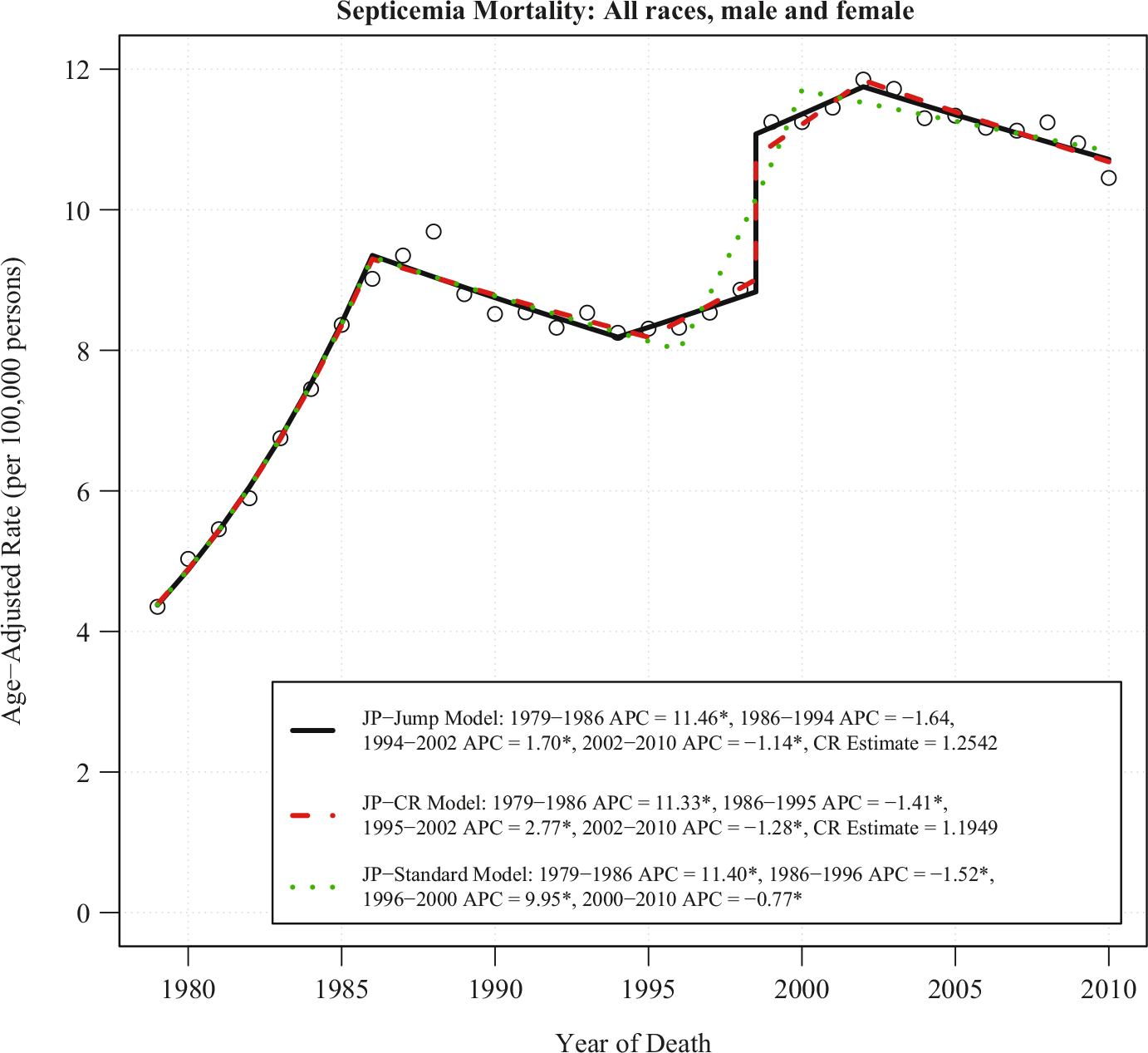
Notes: There are three joinpoints for each model. The estimate of the comparability ratio from JP-Jump Model is 1.2542 with standard error = 0.032. The published comparability ratio is 1.1949 with standard error = 0.002. Both estimated and published comparability ratio are statistically different from one at level 0.05. The symbol * is shown if the annual percent change (APC) is significantly different from zero at level 0.05.

To account for the coding change, both JP-Jump and JP-CR models are applied to the data. The coding change is placed at 1998.5 to represent that 1998 is coded using ICD-9, and 1999 is coded using ICD-10. Figure 1 shows these two methods have similar results. The location of the joinpoints in the two models are identical, except for the end of the second segment, which ends at 1994 for the JP-Jump model and 1995 for the JP-CR model. Both the JP-Jump and the JP-CR model capture an upward trend from 1994/1995 to 2002; but unlike the JP-Standard model, the upward trend only shows a modest increase. The APC for the last segment (2002–2010 for both models), which is the most important segment, is nearly identical: 21.14% per year for the JP-Jump model and 21.28% per year for the JP-CR model; both are statistically significant. The model-based comparability ratio $\widehat{\rho }$ estimated from the JP-Jump model is 1.2542 with a standard error (SE) of 0.032, compared with the published comparability ratio C (C = 1.1949 with SE = 0.0042). Both the estimated and published comparability ratio are statistically different from one at level 0.05.

3.1.2. Melanoma Mortality With Code Changes From ICD-9 To ICD-10

While some causes of death other than cancer have large ICD-9/ICD-10 coding changes, most causes of death due to cancer tend to have relatively small comparability ratios – most have comparability ratios hovering around 0.99 and 1.01 (Anderson et al. 2001), and among the 52 cancer sites published in NCI’s Cancer Statistics Review (Noone et al. 2018), only ten sites have comparability ratios that fall outside of the [0.99, 1.01] range. Until now, a common practice in cancer surveillance is to use the regular Joinpoint model (JP-Standard) to fit the data. For the majority of cancers, this common practice works fine due to the small comparability ratio. However, in a few cases it is possible that even a relatively modest comparability ratio can change the overall conclusions about the trends.

Figure 2 shows the mortality due to melanoma for all races, both males and females combined analyzed from 1992 to 2014 by the JP-Jump, JP-CR, and JP-Standard models. The published ICD-9 to ICD-10 comparability ratio for melanoma is 0.9677, with SE = 0.0032 and 95% CI = (0.9614, 0.9741). The JP-Standard model finds no joinpoint and shows a flat trend with a non-significant APC of 20.06% per year. The JP-CR model with the relevant comparability ratio (0.9677) finds a joinpoint in 2010 with a significant rise of 0.30% per year prior to 2010 and a significant fall from 2010 to 2014 of 1.43% per year. The JP-Jump Model estimates a similar comparability ratio of 0.9444 (SE = 0.0116 and 95% CI = (0.9218, 0.9671)) and finds a joinpoint at 2009 with a significant rise of 0.50% per year prior to the joinpoint, and a significant decline of 1.19% per year after the joinpoint. Despite the small comparability ratio size, these model results are qualitatively different when the coding change from ICD-9 to ICD-10 is taken into account; it produced biased trends when the coding change is not accounted for (using the JP-Standard Model). The JP-Jump model is able to pick up approximately the same modest jump as the JP-CR model, which is estimated by using external data.

Fig. 2. JP-jump model, JP-CR model and JP-standard model of melanoma US mortality rates for all races and both genders, 1992–2014.

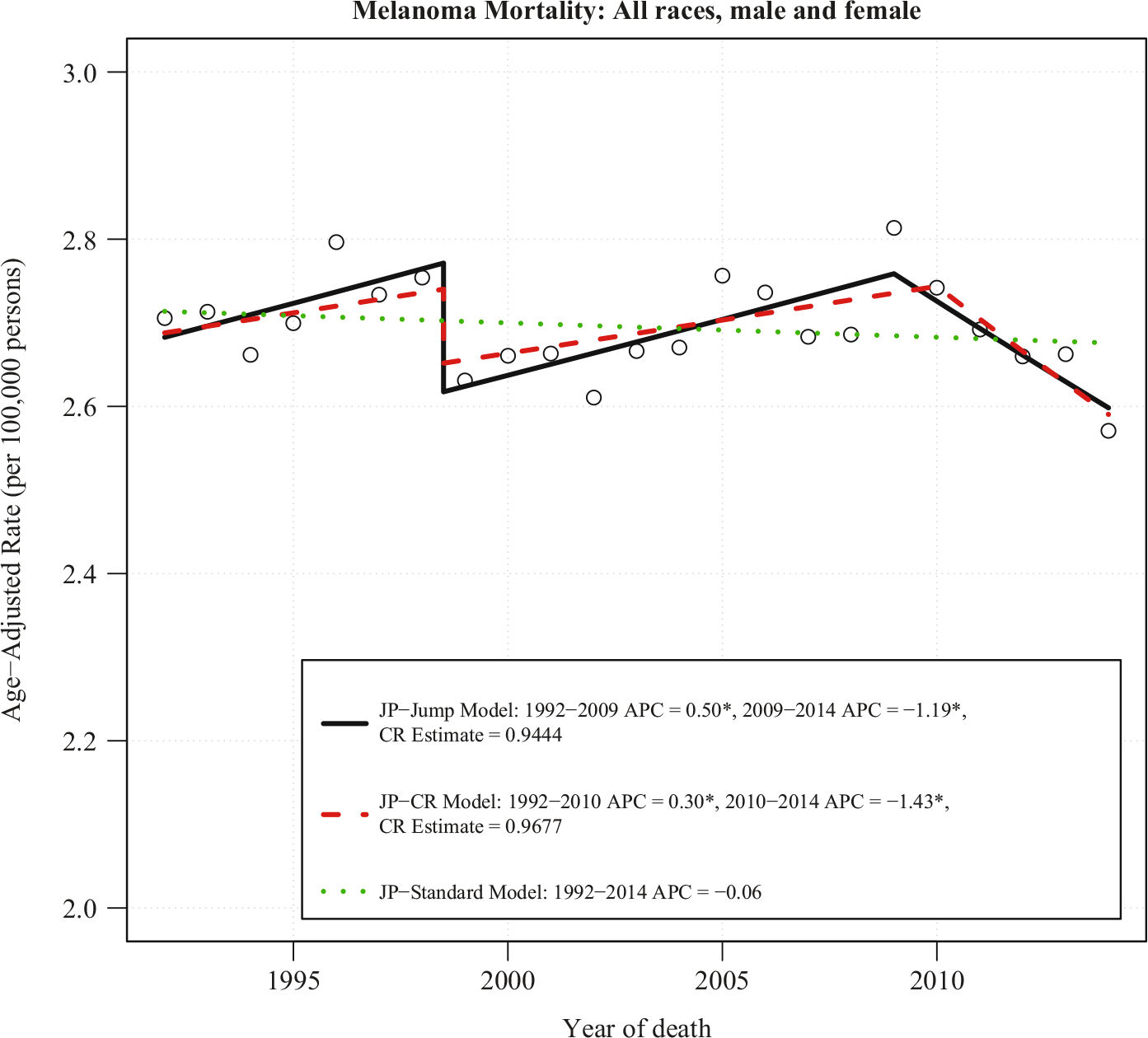
Notes: There is one joinpoint for JP-Jump Model, one joinpoint for JP-CR Model, and no joinpoint for JP-Standard Model. The estimate of the comparability ratio from JP-Jump Model is 0.9444 with standard error = 0.0116. The published comparability ratio is 0.9677 with standard error = 0.0032. Both estimated and published comparability ratio are statistically different from one at level 0.05. The symbol * is shown if the annual percent change (APC) is significantly different from zero at level 0.05.

3.2. Cancer Staging: Summary Staging 2000 and SEER Historical Staging

Analysis of cancer data incidence trends requires consistent staging algorithms across time periods. This can be difficult because staging algorithms change over time to reflect changes in our understanding of disease and changes in prognosis for various subgroups who may be benefitting from new targeted therapies. The National Cancer Institute’s Surveillance Epidemiology and End Results (SEER) cancer registry program started in 1973, and has a series of nine registries covering approximately 10% of the US population since 1975 (more registries have been added in later years). While there are various staging systems in use, the SEER Historical Staging System has been consistent since the program’s inception. Summary Staging 2000 is another staging system, but it can only consistently code back to cases diagnosed in 1998. Both staging systems code cancers as “local”, “regional”, or “distant”. It is of interest to estimate a single trend using the older Historical Staging from 1975 through 1997 and switch over to the more contemporary Summary Staging 2000 in 1998 using the JP-Jump model or JP-CR model. Cases from 1998 onward have been coded using both staging systems, making it possible to compute a comparability ratio.

Figure 3 plots the age-adjusted incidence rate for all races, female, breast cancer at the “distant” stage. The Historical Staging series are plotted from 1975 to 2014 (the most recent year currently available), while the Summary Staging series are plotted from 1998 to 2014. The large gap between these staging systems is due to inflammatory carcinoma being changed from “distant” to “regional” disease, as the improving prognosis of this cancer subtype. Despite this change in coding, incidence rate trends from the two coding systems appear approximately parallel. In order to apply the JP-CR model, we first find the ratios between the Summary Staging 2000 rates and the SEER Historical Staging rates from 1998 to 2014. The mean of these ratios are CR = 0.8059 and the variance of CR = 0.00056, which represents about 20% reduction of incidence rates in the “distant” stage coded by the Summary Staging 2000 when compared to the Historical Staging. Figure 4 consists of data from Historical Staging before 1998 and Summary Staging 2000 from 1998 forward. Both JP-Jump and JP-CR models are fitted to the data. The estimated comparability ratio from the JP-Jump model is 0.7871, which is close to the pre-determined CR = 0.8059, and significantly different from one. The fitting illustrates a continuing flat trend (APC close to 0, not statistically significant) between 1975 to 2002, a drop in 1998 in the incidence rate due to difference between the Historical Staging and Summary Staging 2000 from 1998, and an increasing trend starting from 2002.

Fig. 3.

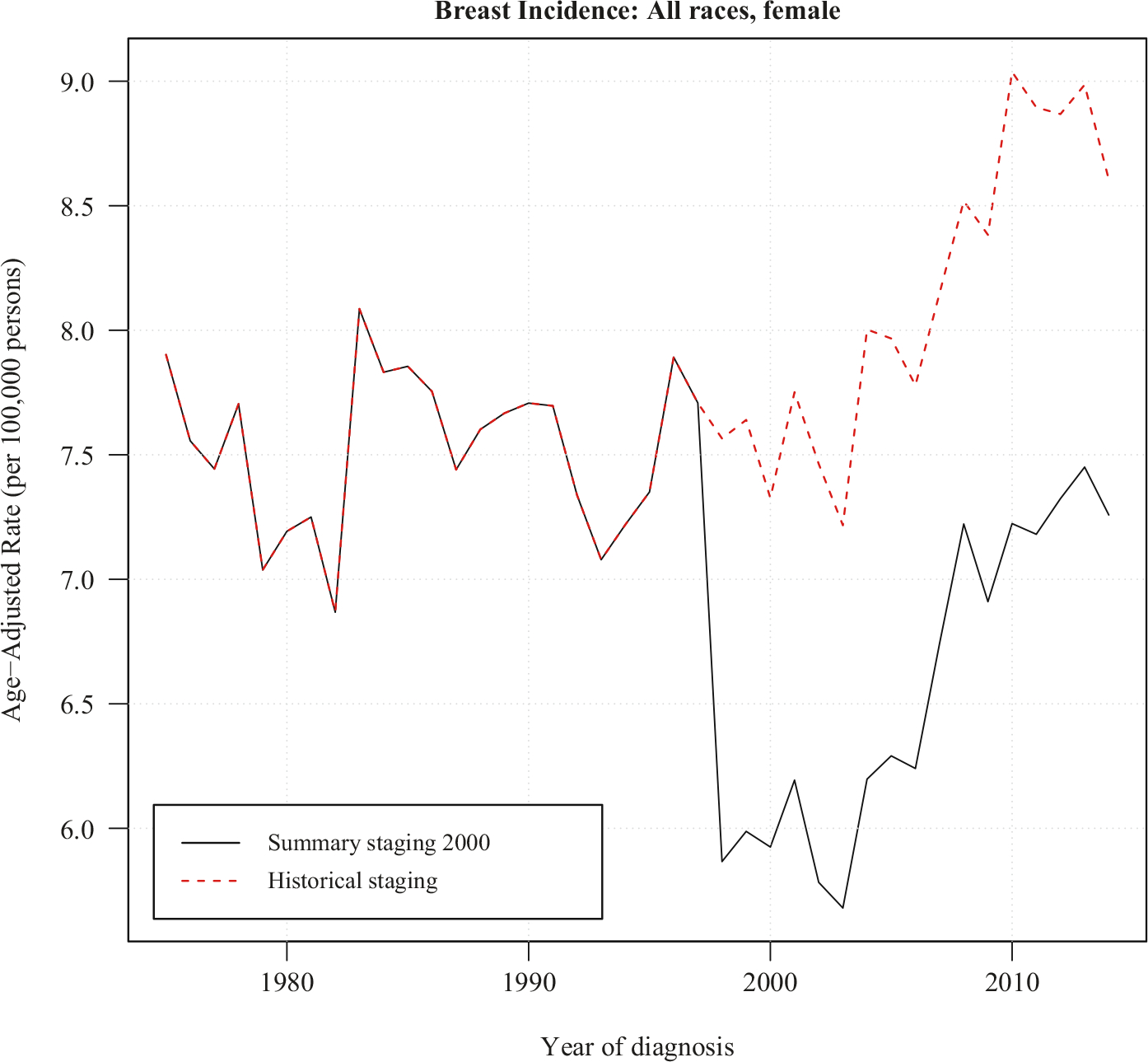
Data of breast cancer incidence rates at distant stage for all races female. The historical staging series has data from 1975 to 2014. Between 1998–2014, the summary staging 2000 series is plotted against the historical staging.

Fig. 4. JP-jump model, JP-CR model and JP-standard model of breast incidence rates for all races female at distant stage using historical staging between 1975–1997 and summary staging 2000 between 1998–2014.

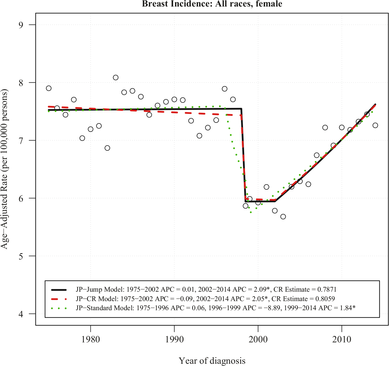
Notes: There is one joinpoint for JP-Jump Model, one joinpoint for JP-CR Model, and two joinpoints for JP-Standard Model. The estimate of the comparability ratio from JP-Jump Model is 0.7871 with standard error = 0.0279, while the comparability ratio calculated from original data is 0.8059, with standard error = 0.0237. Both estimated and calculated from original data comparability ratio are statistically different from one at level 0.05. The symbol * is shown if the annual percent change (APC) is significantly different from zero at level 0.05.

For comparison, the fitted plot from JP-Standard model shows a downward trend with APC = −8.89% per year between 1996 and 1999, which covers the time point of coding system change in 1998. Both the JP-Jump model and the JP-CR model capture the real trends. The Summary Staging 2000 has APC = 2.05% per year for the JP-CR model and APC = 2.09% per year for the JP-Jump model in 2002–2014 – both statistically significant. A possible reason behind the upward trend of incidence rates starting from 2002 could be due, at least in part, to improvements in diagnostic technology, such as the broad use of pet scans since 2002. These more sensitive scans can find sites of distant disease that would have not been apparent in earlier technologies. The finding is consistent with the report of a statistically significant increase in the incidence of breast cancer with distant staging for women aged 25–39 years (Johnson et al. 2013).

4. Discussion

In this article, we propose two approaches – the JP-Jump and JP-CR models – to model trends in data when there is a coding change. There are several practical issues to consider when selecting the most suitable model.

To analyze trend data when a coding change occurs, assuming a comparability ratio based on double coding using the new and old codes is available, any one of the three models (JP-Jump, JP-CR, or JP-Standard model) may be applicable. In many cases, one may find that all three models produce virtually identical results, especially when the CR from the double coding is small (e.g., between 0.99 and 1.01), denoting little effect of the coding change. If no CR is available, then only the JP-Jump model or the JP-Standard model are appropriate. Which method to use in practice often depends on several factors, such as size of the data cohort, and size and variability of the CR ratio.

In comparing the three methods, the estimates of trends from the JP-Standard model can be biased when coding changes are not taken into account, even if the jumps are modest. The first two methods can yield similar results, but the JP-Jump model has advantages over the JP-CR model because there is no requirement to know the size of the jump prior to applying the model. Even if double coding is available and the ratio between the two codes can be estimated, the JP-CR model may not be suitable for practical use in cases where the statistical variability of the CR is high or the accuracy or applicability of the estimate is questionable. Sampling error or small numbers may result in unstable CRs. Also, demographic and geographic variation in the CR may make the applicability of a CR for all races, or for all states, problematic when analyzing data by demographic groups or states. In contrast, the JP-Jump model has advantages because it is always estimated directly using the data series of interest, that is, it can adapt data to estimate the size of jump and the trend simultaneously, for each subgroup or for the whole group.

However, like the regular Joinpoint model, the JP-Jump model is sensitive to the data and the location of the joinpoints, and results should be interpreted with caution. Estimates of jump sizes, particularly when close to a joinpoint, might be confounded with the slopes before and after the joinpoint itself. Furthermore, the underlying data variability may make estimation of a small or modest jump size impossible. For small subpopulations (e.g., Asian/Pacific Islander, American Indian/Alaska Native, rare cancer sites, or small geographic areas), such situations may occur. In the JP-Jump model, one can check that the jump is statistically different from zero. We note that in cases where the jump size is not statistically significant, the JP-CR model may be the better choice, and that even with statistical significance one should be wary of the data variability as compared to data set size when assessing results of the JP-Jump model. Overall, we suggest applying both models to data sets to consider the best fit for particular scenarios. In many cases where the estimates are similar, the JP-Jump model may be preferred due to its specificity per data set.

The JP-Jump model has a similar form to the regular Joinpoint model. The model fitting and inference on the parameters are derived by modification from those of the regular Joinpoint model. Note that the regular Joinpoint model has a continuous mean function, while the mean function of the JP-Jump model is continuous only at places other than the jump location. Additionally, we assume in the JP-Jump model that the location of the jump is known, and only one such jump is allowed. A direct extension to the JP-Jump model is to allow more than one known jump in response to multiple coding changes over time. The implementation of such a model is straightforward, although with more than one coding change one has to be especially careful about the issue of confounding between the APC of segments and the size of the jump.

In the JP-Jump model (Equations (2)), the errors ϵ_i are assumed to be independent N(0, σ²). Just like the regular Joinpoint model, these assumptions can be relaxed to allow correlated errors and non-constant variance. The model fitting and inference procedures can be extended from the regular Joinpoint model as well.

In summary, trend data with a sudden jump occurs in many situations, particularly in health data, where coding systems and practices change over time. Analyses using the regular Joinpoint model that ignore these jumps could produce misleading conclusions, as shown in the melanoma mortality example. The proposed methods in this article incorporate a sudden discontinuous jump in an otherwise continuous joinpoint model. In particular, the JP-Jump model can estimate the magnitude of the jump, while at the same time can find the change-points of the continuous trend. The methods provide a useful tool for trend analysis.