Data driven estimation of novel COVID-19 transmission risks through hybrid soft-computing techniques

Abstract

Coronavirus genomic infection-2019 (COVID-19) has been announced as a serious health emergency arising international awareness due to its spread to 201 countries at present. In the month of April of the year 2020, it has certainly taken the pandemic outbreak of approximately 11,16,643 infections confirmed leading to around 59,170 deaths have been recorded world-over. This article studies multiple countries-based pandemic spread for the development of the COVID-19 originated in the China. This paper focuses on forecasting via real-time responses data to inherit an idea about the increase and maximum number of virus-infected cases for the various regions. In addition, it will help to understand the panic that surrounds this nCoV-19 for some intensely affecting states possessing different important demographic characteristics that would be affecting the disease characteristics. This study aims at developing soft-computing hybrid models for calculating the transmissibility of this genome viral. The analysis aids the study of the outbreak of this virus towards the other parts of the continent and the world. A hybrid of wavelet decomposed data into approximations and details then trained & tested through neuronal-fuzzification approach. Wavelet-based forecasting model predicts for shorter time span such as five to ten days advanced number of confirmed, death and recovered cases of China, India and USA. While data-based prediction through interpolation applied through moving average predicts for longer time spans such as 50–60 days ahead with lesser accuracy as compared to that of wavelet-based hybrids. Based on the simulations, the significance level (alpha) ranges from 0.10 to 0.67, MASE varying from 0.06 to 5.76, sMAPE ranges from 0.15 to 1.97, MAE varies from 22.59 to 6024.76, RMSE shows a variation from 3.18 to 8360.29 & R² varying through 0.0018 to 0.7149. MASE and sMAPE are relatively lesser applied and novel measures that aimed to achieve increase in accuracy. They eliminated skewness and made the model outlier-free. Estimates of the awaited outburst for regions in this study are India, China and the USA that will help in the improvement of apportionment of healthcare facilities as it can act as an early-warning system for government policy-makers. Thus, data-driven analysis will provide deep insights into the study of transmission of this viral genome estimation towards immensely affected countries. Also, the study with the help of transmission concern aims to eradicate the panic and stigma that has spread like wildfire and has become a significant part of this pandemic in these times.

1. Introduction

The World Health Organization (WHO) as on January 30, 2020 has announced 2019–2020 corona-genomic-virus a public health-emergency of international concern that can be abbreviated as PHEIC. Situation further worsened worldwide which was declared pandemic on March 11, 2020. Till now, local transmission of this epidemic is being recording and increasing the count in countries including the six WHO regions.

Basically, their structure observed so far can be described as enveloped non-segmented positive-sense RNA-genomic viruses having place in the clan of Corona viridae majorly circulated in humans with other mammals. However, in most cases studied, individual related coronavirus infections are mild having identified two Beta corona viruses: severe-acute-respiratory-syndrome-coronavirus (SARS-CoV) & Middle-East-respiratory-syndrome-coronavirus (MERS-CoV) (Figs. 1 and 2 ).

Fig. 1.

Detailed diagram of COVID-19 affecting the host RNAs.

Fig. 2.

COVID-19 symptoms & transmission as directed by CDCP/USA Today/WHO.

The outburst of nCOVID-19 studied in detail through data-based modeling & forecast analysis [1]. Detailed explanation of mathematical perspective to understand spread of infectious diseases is provided [2]. Estimation of atmosphere pollutants through dynamic indicators, discussion of the meditating body complexity, statistical simulations towards dynamics of HIV, IoT-based wireless transmissions having malware spread were modelled and studied in detail [3], [4], [5], [6]. Coronavirus data analyzed for risk assessment and forecasts [7]. Transmission data of the virus outbreak to atudy gov interventions [8]. Towards tracking the rate of transmission of epidemic based on the data driven study of the situation was carried out [9]. Study of a mathematical model towards dynamics of transmission and its control provided [10]. Spatial spread relationships during Coronavirus pandemic spread into the world via self- organizing maps analyzed [11]. WHO report on novel coronavirus in Japan and MERS-CoV update has been surveyed [12], [13]. WHO report on Coronavirus updated on January 19, 2020 [14]. The rate of spread of the epidemic in the scale-free networks [15]. As per the outcomes of this pandemic, efficiency of control strategies towards reduction of social mixing in China is modelled [16]. The complexity in the forecast accuracy of nCOVID-19 pandemic is dealt with [17]. Futuristic estimations computed via supervised learning of COVID [18]. Time series forecasting of the genomic virus spread in India applying genetic programming [19]. This pandemic outbreak is studied on the basis of training testing of Multimodal data [20]. The molecules that may perhaps enter into host cell and cause acute respiratory syndrome targeting towards coronavirus studied [21]. Study forecasted impending COVID-19 spread cases for China plus some other regions using mathematical & traditional time-series prediction models [22]. Mathematical model-based prediction at an early stage achieved for the outburst of this particular virus in China [23]. Extensive exploration of pneumonia outbreak via corona-genome originating from bat species [24].

None of the authors have studied the wavelet based neuronal fuzzification hybrid model for the data of country-wise spread of COVID-19 genome. In this article, forecasts of the country-based day to day basis data of confirmed, deaths and recovered cases. Analysis has been carried out through the machine-learned WNF hybridization predicting for shorter time span and forecasts through interpolation alongwith moving averages method for longer time spans and performance measures through MASE and sMAPE which have not been applied in any of the studies yet.

2. Dataset assessment

Single variable involving time successions’ datasets have to be collected for real-time response variables’ estimation for nCOVID-19 records in India, China and the USA. Now, such cases from three diverse countries having totally different history about their past cases have been simulated. Further, in case of India & USA, we have considered the daily laboratory-confirmed records starting approximately from mid of January through May 17, 2020 with variations in time-periods according to different datasets for model computations. Daily COVID-19 confirmed, deaths and recovered cases data for China are taken for the time period December 31, 2019 through May 17, 2020; daily corona spread in India having confirmed cases from January 31, 2020 through May 17, 2020, deaths cases February 22, 2020, through May 17, 2020, respectively. The dataset for India contains a total of 108 observations, 119 observations for USA, 139 observations for China. For these countries the outbreaks of nCoV-19 started at absolutely different timeline and the epidemic curves for India & USA majorly not showing any kind of diminishing curve or trajectory as per the response variables, alike China. A pragmatic approach assumes that the trend will continue indeterminately in the future which is very different from various deterministic modeling methods that would perhaps tend towards convergence at farther future.

During exploration, daily data sets of China from December 31, 2019 to May 17, 2020 (a total of 139 days); for India from January 31, 2020 to May 17, 2020 (a total of 108 days) and for USA from is taken from January 20, 2020 to May 17, 2020 (a total of 119 days) trusted data sources provided by designated authorities. These three datatypes have been further divided into three data sets: Confirmed cases, Deaths cases and Recovered cases respectively as mentioned in Table 1 . From the sample of each data set taken separately for the prediction simulation, first 4 used as input values and rest is used to train and test the forecast model. As in from the sample of 139 days data, first four used as input values and rest 115 used to train the model and 20 data values to test the hybrid prototype. Similarly, from the sample of 108 days data, first four used as input values and rest 84 used to train the model and 20 data values to test the hybrid prototype and from the sample of 119 days data, first four used as input values and rest 95 used to train the model and 20 data values to test the hybrid prototype. Similarly, for various time spans the data has been divided on the aforesaid format.

Table 1.

Data sets for simulation for prediction models.

Data	Recorded Cases	Time span under consideration
		From	Up to
Data type-1: China	Confirmed cases	December 31, 2019	May 17, 2020
	Deaths cases	December 31, 2019	May 17, 2020
	Recovered cases	December 31, 2019	May 17, 2020
Data type-2: India	Confirmed cases	January 31, 2020	May 17, 2020
	Deaths cases	February 22, 2020	May 17, 2020
	Recovered cases	February 26, 2020	May 17, 2020
Data type-3: USA	Confirmed cases	January 20, 2020	May 17, 2020
	Deaths cases	February 22, 2020	May 17, 2020
	Recovered cases	March 9, 2020	May 17, 2020

3. Soft-Computing techniques

3.1. Wavelet decomposition

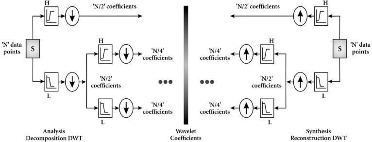
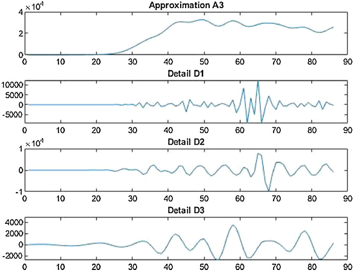
Conversion function is a function that converts a waveform into various rate of recurrence constituents. If conversion function is used in agreement with the scale then it is called wavelet transform, which converts the function alongwith the interval realm into the rate of recurrence realm. Wavelet decomposition is carried out for records handling as with the help of wavelet demonstration, the non-stationarity of the economic and financial time series can be explained (Figs. 3 and 4 ).

Fig. 3.

Detailed structure of analysis and synthesis of DWT.

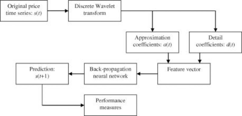
Fig. 4.

Flowchart of DWT procedure.

Theorem: Wavelet is a blend of sine-cosine waves containing characteristics that would vary around zero plus remains restricted into interval domain. Wavelet-function is classified as: the father wavelet (ϕ) - mother wavelet (ψ) possessing following characteristics:

$${\int }_{-\infty }^{\infty }\varphi \left(x\right)dx=1and{\int }_{-\infty }^{\infty }\psi \left(x\right)dx=0$$

Remark: Integration of amplified dyadic alongwith integral transformations, mother-father wavelets are changed into the wavelet clan:

$${\varphi }_{j,k}\left(x\right)=2^{j/2}\varphi (2^{j}x-k)and{\psi }_{j,k}\left(x\right)=2^{j/2}\psi (2^{j}x-k)$$

3.2. Neuronal-Fuzzification procedural aspect

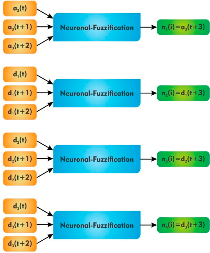
Neuronal-Fuzzification procedures have been premeditated to comprehend the fuzzy reasoning procedure and the weights connecting in the network which need to be allied with fuzzy reasoning constraints involving the backpropagation knowledge. This identifies fuzzy measures, learn the connexion function for fuzzy reasoning. The neuronal-fuzzy model initiated with decoding the membership assessment of each with the aid of Fuzzy C-Means, trailed through fuzzified inference steps (Fig. 5 ).

Fig. 5.

Flowchart of application of Wavelet decomposed data into Neuronal-Fuzzification .

4. Performance errors in forecasting

4.1. Mean absolute error (MAE)

Theorem: Absolute value for altercations in between original calculations and estimated values through the simulation of mean of these sums of absolute errors. Also, here we consider that each of the individual errors attain equivalent weights referred to as Mean Absolute error.

Remark: This mean absolute error is denoted as:

$$MAE=\frac{1}{N}\left(\sum _{i=1}^N|d_i-y_i|\right),$$

d denoted the actual quantity; y denotes the anticipated assessment; N- no. of days in prediction.

Algorithm to find value of Mean Absolute Error:

• 1Compute regressive line as: y= axe+b, a & b:- real constants.
• 2Introduce X values in the linear regression equality determining the new values, Y’.
• 3Measure difference of new predicted value from actual measurement to catch the error.
• 4Take absolute value of the errors.
• 5Add up the calculated values obtained in Step 4.
• 6Finding mean.

4.2. Root mean squared error (RMSE)

Theorem: The root mean squared error is square root for Mean Squared Errors calculated via actual outcomes and the expected quantities.

Remark: $RMSE=\sqrt{\frac{\sum _{i=1}^n{(y_i-{\widehat{y}}_i)}^2}{n}}$ ;y_i denotes actual quantity; ${\widehat{y}}_i$ denotes predicted outcomes; n is no. of days of estimation.

Algorithm to find the value of Root Mean Squared Error:

1. Find the regression line: y=axe+b, a and b are real constants.

2. Introduce X assessments in the linear lapse equality for computing new assessments, Y’.

3. Measure subtraction of new Y assessment from the original to calculate the inaccuracies.

4. Squaring inaccuracies.

5. Summation of inaccuracies.

6. Discovering the mean.

7. Take the square root of mean.

4.3. Goodness of fit (R²)

Theorem: calculates the proportion in the dependent variable that is simulated by linear lapse and the predictor variable which is the independent variable. It defines the degree of evaluation ability of a model to envisage or explain an outcome for linear lapse model.

Algorithm to determine the goodness of fit:

1. Find regressive line (curve): y=axe+b, a and b are real constants.

2. Compute sum of squared errors for regression setup, $SSE=\sum _{i=1}^n{(y_i-{\widehat{y}}_i)}^2$

3. Also, compute sum of squared errors of the baseform setup, $SST=\sum _{i=1}^n{(y_i-{\overline{y}}_i)}^2$

4. Calculate the ratio: SSE/SST.

5. Subtract the ratio from 1. i.e. $R^2=1-\frac{SSE}{SST}$

4.4. Symmetric mean absolute percentage error (sMAPE)

Theorem: A percentage-based error to accurately measure the relative errors on percentage basis. This performance measure proposes a lower and upper bound to the errors in the range 0% to 100%.

Remark: It is purely based on differences of actual responses and predicted responses recorded by the forecasters. Simulated through the formulae:

$$\begin{array}{c}sMAPE=\frac{100\%}{N}\sum _{p=1}^N\frac{|{\widehat{Y}}_p-Y_p|}{|Y_p|+|{\widehat{Y}}_p|}\hfill \\ where\hfill \\ {\widehat{Y}}_p-\text{Estimated}\text{simulated}\text{values}\hfill \\ Y_p-\text{Original}\text{simulated}\text{values}\hfill \\ p-\text{fitting}\text{point}\hfill \\ N-\text{number}\text{of}\text{fitting}\text{points}\hfill \end{array}$$

Outcome of this computation can be seen as at every fitting point, p divided again by number of fitting points, N. It was first proposed by Armstrong and later modified applied by Flores. This absolute error analyses statistical performance of the model via significant symmetry and unbiases. Applying these measures into the forecasters resembles directly to geometric mean.

4.5. Mean absolute scaled error (MASE)

Theorem: Based on Mean Absolute Error performances of the model constructed, MASE stands independent of the scale of the data which means it could be applied towards comparing forecasts in various datasets irrespective of their scales.

Remark: Simply, it can be understood as the MAE of the actual forecast divided by the MAE of the naïve forecast which is simulated on the in-sample data. For a non-seasonal timeseries, represented through the formula:

$$\begin{array}{c}MASE=\frac{\frac{1}{N}{\sum }_i|e_i|}{\frac{1}{P-1}{\sum }_{p=2}^P|Y_p-Y_{p-1}|}=\frac{MA{E}_{actual}}{MA{E}_{naivein-sample}}\hfill \\ where\hfill \\ |e_i|=|{\widehat{Y}}_i-Y_i|\hfill \\ {\widehat{Y}}_p-\text{Anticipated}\text{assessment}\text{values}\hfill \\ Y_p-\text{Actual}\text{simulated}\text{values}\hfill \\ p=1...,P\hfill \\ N-\text{number}\text{of}\text{forecasts}\hfill \end{array}$$

First proposed by Hyndman and Koehler, it is scale-independent, symmetrical, outliers resistant and an applicable measure to maintain predictability accuracy. It determines the comparative forecasting accuracy.

5. Generation of hybrid WNF prototype

5.1. Application and results

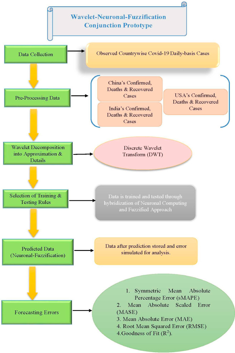
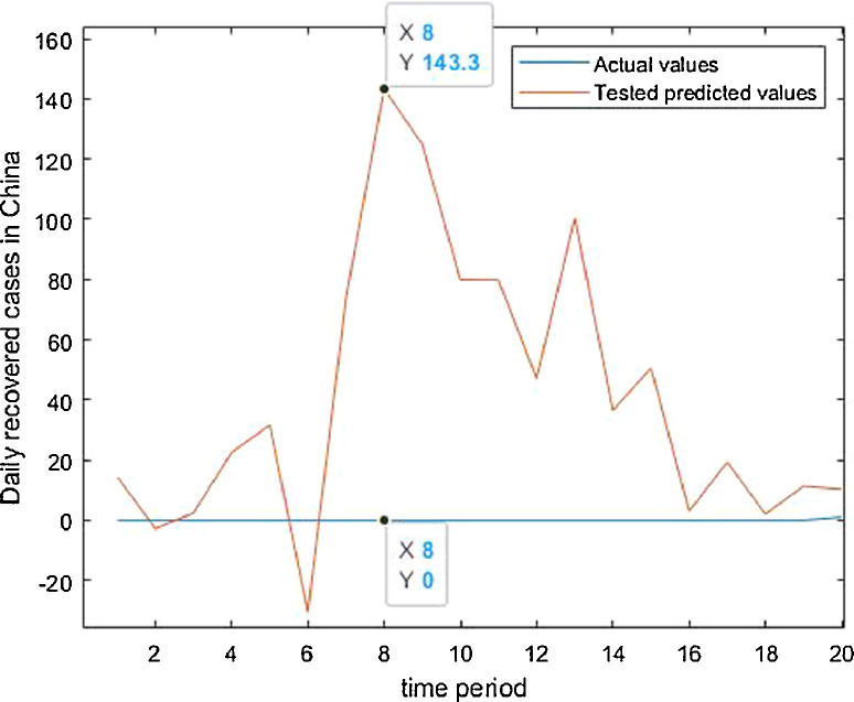
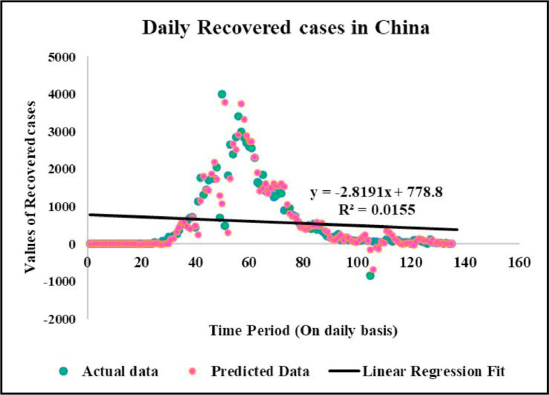
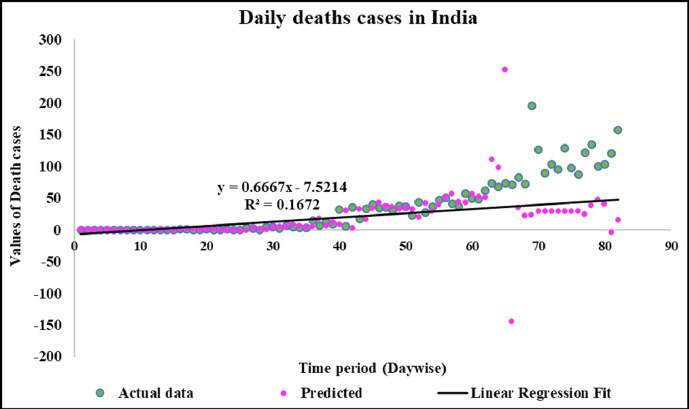
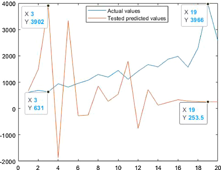
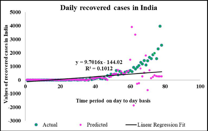
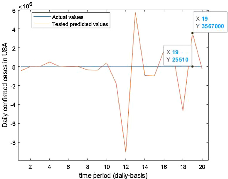
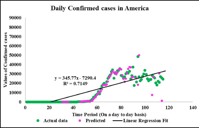
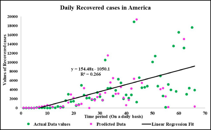
Neuronal setup gets trained and tested through fuzzification having hybrid method for simulation of training and testing. Sugeno inference-rules on loop for 500 epochs having strictly zero error-tolerance levels. Estimating technique includes noise filtered as per Wavelet decomposition that extracts characteristics trained & tested to forecast the predictor variables (Fig. 6 ). WNF designed for Country based data of Corona positive cases for the time period spanning approximately from December 31, 2019 uptil May 17, 2020 on a daily basis is considered. The large amount of data being recorded everyday gets trained, tested and modeled through Wavelet-Neuronal fuzzified prototype. This computation studied the scenario of countries such as China, India and USA for three major divisions that are Daily Confirmed cases, Daily deaths cases and Daily recovered cases as per the data statistics. Table 2 tabulates the simulization errors in prediction of Country-wise Covid-19 daily cases’ data. The significance levels of China for confirmed, death and recovered cases are 0.25, 0.10, 0.5 respectively; for India having confirmed, death and recovered cases as 0.10, 0.67, 0.00 & for America having confirmed, death and recovered cases as 0.17, 0.50, 0.13 respectively. Further, Mean Absolute Scaled Error (MASE) values of China for confirmed, death and recovered cases are 0.06, 0.99, 0.15 respectively; for India having confirmed, deaths’ plus recovered cases as 5.76, 5.52, 3.11 & for America having confirmed, deaths’ plus recovered cases as 3.39, 1.34, 5.57 respectively. Symmetric Mean Absolute percentage error (sMAPE) values of China for confirmed, deaths plus recovered cases are 1.73, 1.97, 0.60; for India having confirmed, death and recovered cases as 0.15, 0.23, 0.96 & for America having confirmed, death and recovered cases as 0.16, 0.26, 0.74 respectively. Similarly, MAE values for China are 22.59, 33.68, 31.88; India are 486.58, 28.08, 591.98; America having 4411.03, 424.68, 6024.76. RMSE values for China are 24.85, 3.18, 42.16, 622.55, 39.20, 923.56, 6350.69, 506.56 and goodness of fit measure R2 values for China are 0.0801, 0.0018, 0.0155; India are 0.7048, 0.1672, 0.1012; America are 0.7149, 0.5391, 0.266. Table 3 compares various studies using different Intelligent models for the widespread COVID-19 genome pandemic to the present study of the hybrid model. Clearly, MASE and sMAPE prove to be better performance measures as they accurately predicted the errors and have symmetries which eliminated the skewness and made the model outlier resistant. Improved scalability of the data. This improvised the applicability of the model on the virus data.

Fig. 6.

Flowchart of Hybrid WNF Prototype for COVID-19 data.

Table 2.

Simulation errors in prediction of Country-wise Corona daily cases data.

		Statistical error measures
Countries	Types of Cases	Significance level(Alpha)	MASE	sMAPE (%)	MAE	RMSE	R2
China	Confirmed	0.25	0.06	1.73	22.59	24.85	0.0801
	Deaths	0.10	0.99	1.97	33.68	3.18	0.0018
	Recovered	0.5	0.15	0.60	31.88	42.16	0.0155
India	Confirmed	0.10	5.76	0.15	486.58	622.55	0.7048
	Deaths	0.67	5.52	0.23	28.08	39.20	0.1672
	Recovered	0.00	3.11	0.96	591.98	923.56	0.1012
USA	Confirmed	0.17	3.39	0.16	4411.03	6350.69	0.7149
	Deaths	0.50	1.34	0.26	424.68	506.56	0.5391
	Recovered	0.13	5.57	0.74	6024.76	8360.29	0.266

Table 3.

Various studies using different Intelligent models for the widespread COVID-19 genome pandemic.

Year	Author	Description	Parameters	Results
March 2020	Fang Y. et al.	Data-driven analysis of Transmission dynamics of the COVID-19 outbreak	SEIR model, Data fitting, MAE, MSE, R2	MAE=2627.855; MSE=8,800,640.291; R2=0.980963
April 2020	Chakraborty, T; Ghosh, I.	Data-driven analysis of real time forecasts & risk assessment of COVID-19	Arima-WBF; RMSE, MAE, Fitted tree-R2	55.25 ≤ RMSE ≤ 631.91; 40.05 ≤ MAE ≤ 306.78; R2=0.896
May 2020	Salgotra, R. et al	Time-Series Analysis and Forecast of the COVID-19 in India	Genetic Programming; RMSE, R2	5.55 ≤ RMSE ≤ 284.9057; 0.9881 ≤  R2 ≤ 0.9999
June 2020	Rustam, F. et al	COVID-19 Forecasting via Supervised Machine Learning	RMSE; MSE; MAE; R2	2443.48 ≤ RMSE ≤ ,114,547.58; 1827.85 ≤  MAE  ≤ ,106,739.82; 0.02 ≤  R2 ≤ 0.99;
2020	Present study Bhardwaj; Bangia	Wavelet-based neuronal- fuzzification hybrid model for the data of China, India, USA for spread of COVID-19 genome	MSE, MASE, sMAPE, MAE, RMSE, R2 Significance level (alpha)	0.10 ≤ alpha ≤ 0.67; 0.06 ≤ MASE ≤ 5.76; 0.15% ≤ sMAPE ≤ 1.97%; 22.59 ≤ MAE ≤ 6024.76, 3.18 ≤ RMSE ≤ 8360.29 & 0.0018 ≤ R2 ≤ 0.7149

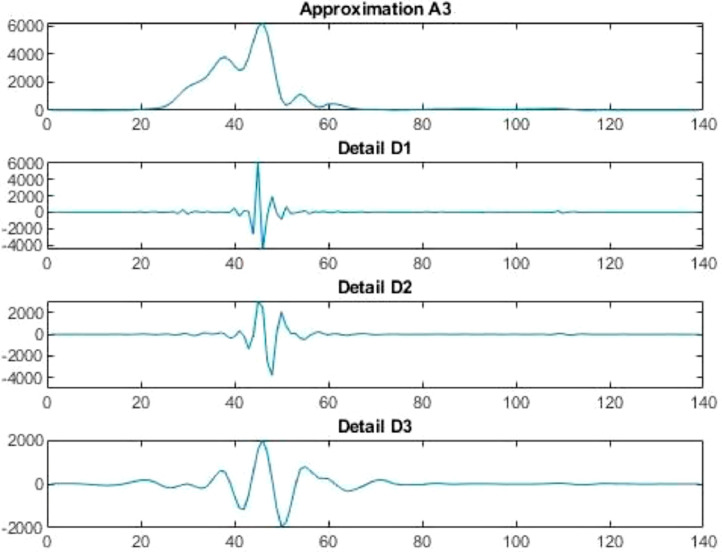
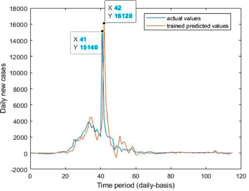
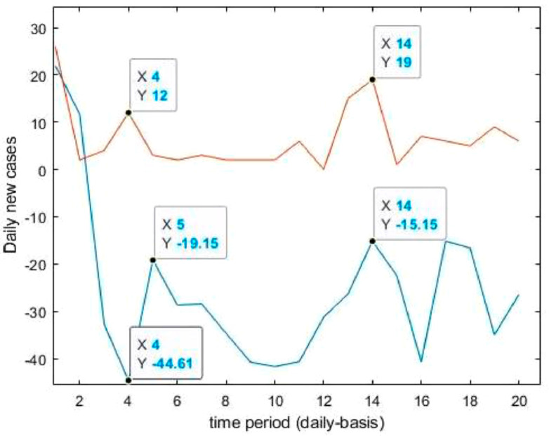
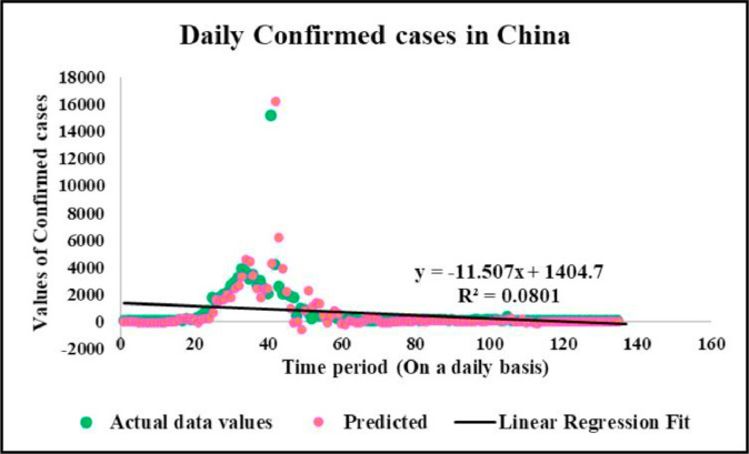
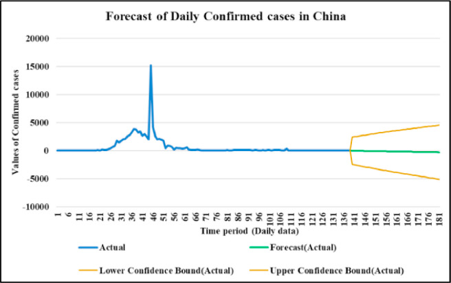
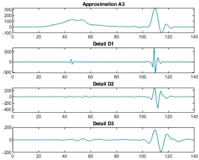
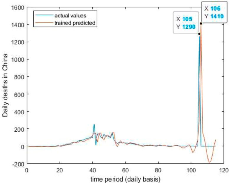
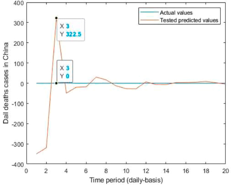
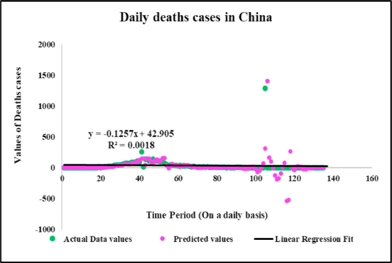
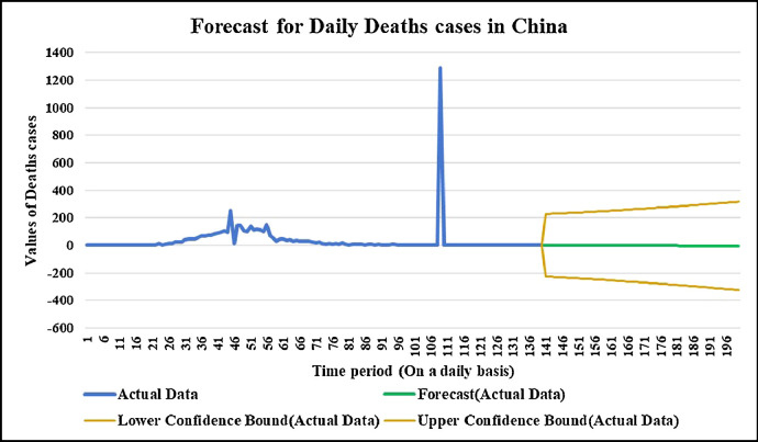
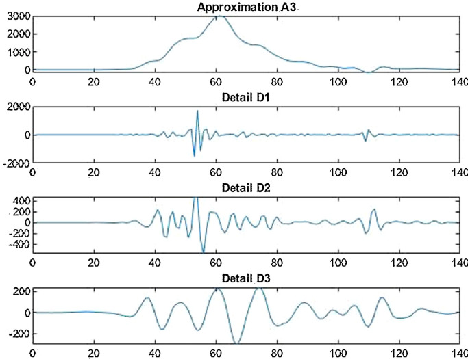
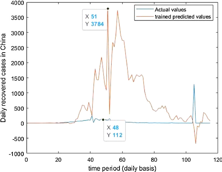
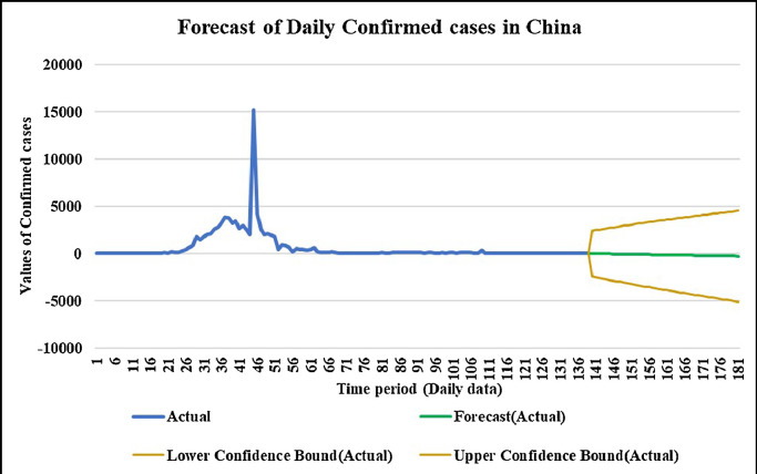
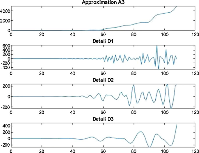
For the country of China, the data has been analyzed under three main distinctions that are: Confirmed cases, Deaths’ cases and Recovery cases that are being recorded every day and provided through public bulletin from designated authorities as depicted through Fig. 7, Fig. 8, Fig. 9, Fig. 10, Fig. 11, Fig. 12, Fig. 13, Fig. 14, Fig. 15, Fig. 16, Fig. 17, Fig. 18, Fig. 19, Fig. 20, Fig. 21 .

Fig. 7.

Wavelet decomposition of daily confirmed cases in China.

Fig. 8.

Trained vs actual data values .

Fig. 9.

Tested vs actual data values.

Fig. 10.

Predicted vs actual data values with linear fit.

Fig. 11.

Forecasting longer time period with the past responses.

Fig. 12.

Wavelet decomposition of daily deaths cases in China.

Fig. 13.

Trained vs actual data values.

Fig. 14.

Tested vs actual data values.

Fig. 15.

Predicted vs actual data values with linear fit.

Fig. 16.

Forecasting longer time period with the past responses.

Fig. 17.

Wavelet Decomposition of daily recovered cases in China.

Fig. 18.

Trained vs actual data values.

Fig. 19.

Tested vs actual data values.

Fig. 20.

Predicted vs actual data values with linear fit.

Fig. 21.

Forecasting longer time period with the past responses.

Case-1: Confirmed Cases in China Daywise (Fig. 7, Fig. 8, Fig. 9, Fig. 10 and 11).

Case-2: Deaths’ Cases in China (Fig. 12, Fig. 13, Fig. 14, Fig. 15, Fig. 16 and 16).

Case-3: Recovered Cases in China (Fig. 17, Fig. 18, Fig. 19, Fig. 20, Fig. 21 and 21).

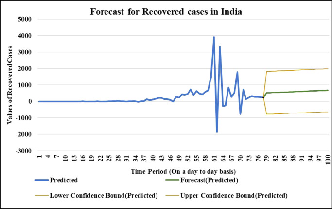
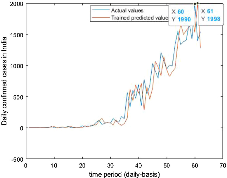
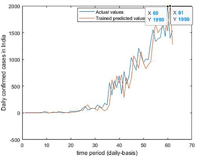
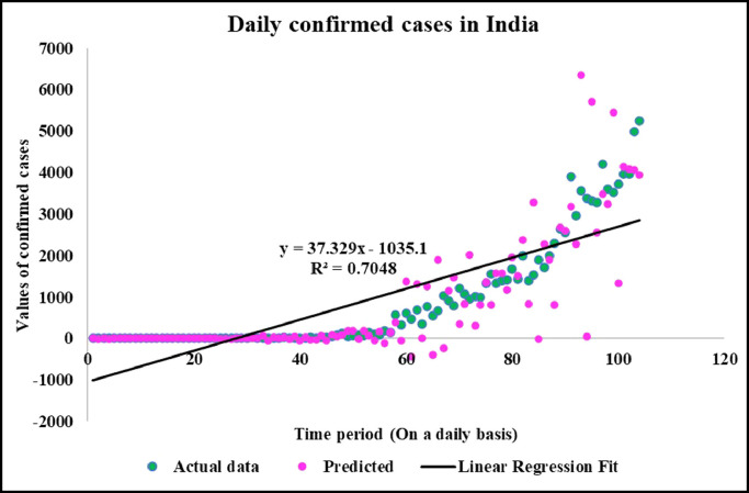
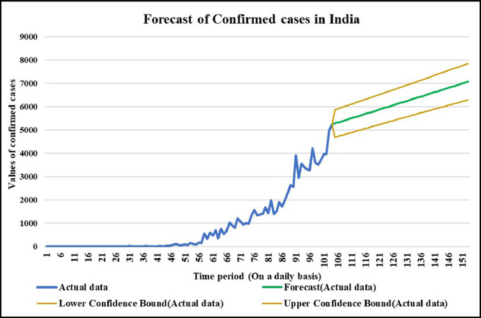
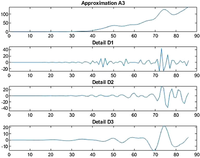
For the country of India, the data has been analyzed under three main distinctions that are: Confirmed cases, Deaths’ cases and Recovery cases that are being recorded every day and provided through public bulletin from designated authorities as depicted through Fig. 22–36 .

Fig. 22.

Wavelet decomposition of daily confirmed cases in India.

Fig. 36.

Forecasting longer time period with the past responses.

Case-1: Confirmed Cases in India Daywise (Fig. 22, Fig. 23, Fig. 24, Fig. 25, Fig. 26 and 26).

Fig. 23.

Trained vs actual data values.

Fig. 24.

Tested vs actual data values.

Fig. 25.

Predicted vs actual data values with linear fit.

Fig. 26.

Forecasting longer time period with the past responses.

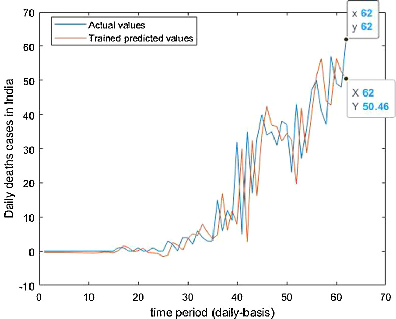
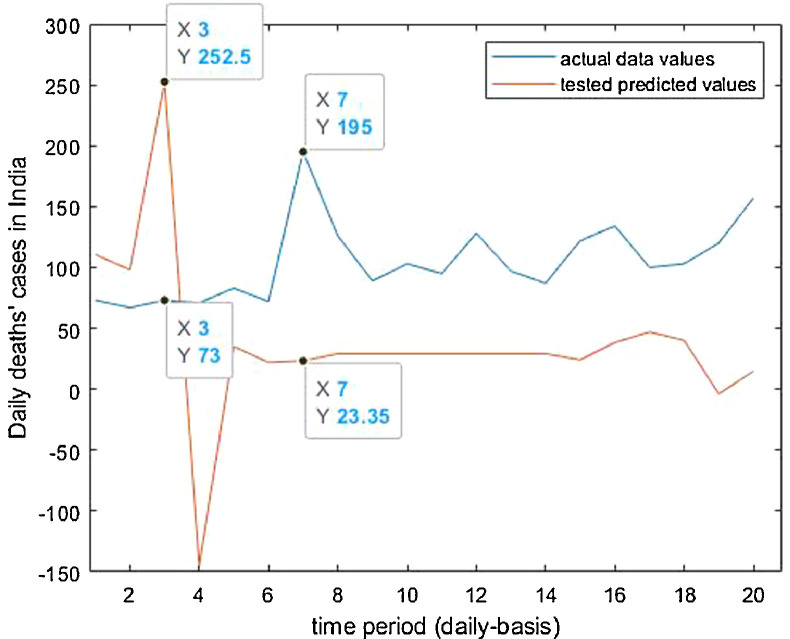
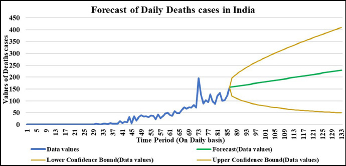
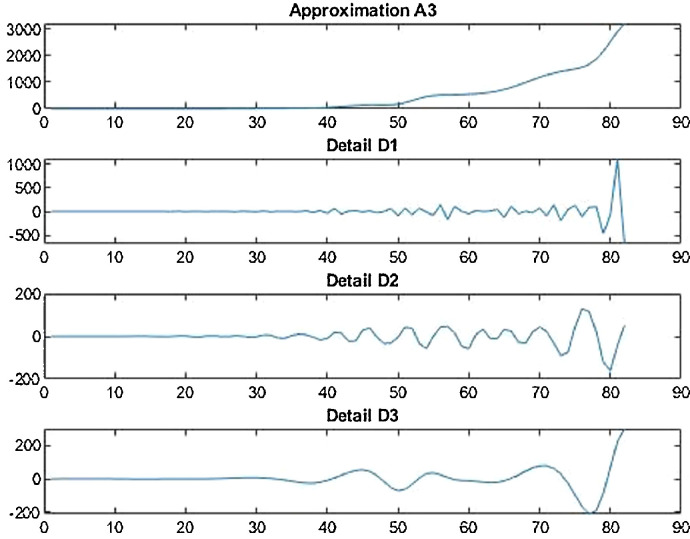
Case-2: Deaths’ cases in India Daywise (Fig. 27, Fig. 28, Fig. 29, Fig. 30, Fig. 31 and 31 ).

Fig. 27.

Wavelet decomposition of daily deaths cases in India.

Fig. 28.

Trained vs actual data values.

Fig. 29.

Tested vs actual data values.

Fig. 30.

Predicted vs actual data values with linear fit.

Fig. 31.

Forecasting longer time period with the past responses.

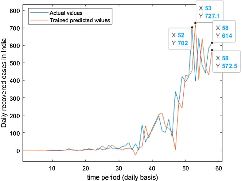
Case-3: Recovered cases in India Daywise (Fig. 32, Fig. 33, Fig. 34, Fig. 35, Fig. 36 and 36 ).

Fig. 32.

Wavelet decomposition of daily recovered cases in India.

Fig. 33.

Trained vs actual data values.

Fig. 34.

Tested vs actual data values.

Fig. 35.

Predicted vs actual data values with linear fit.

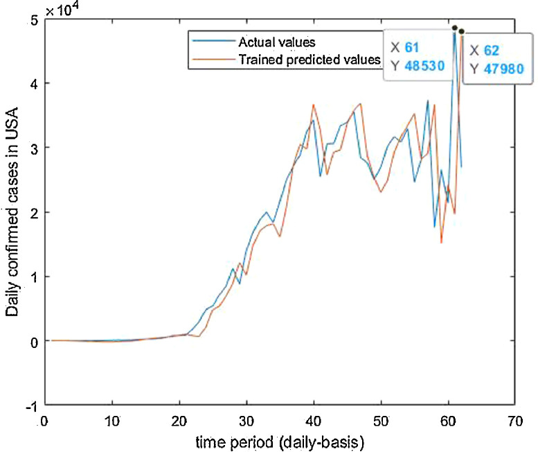
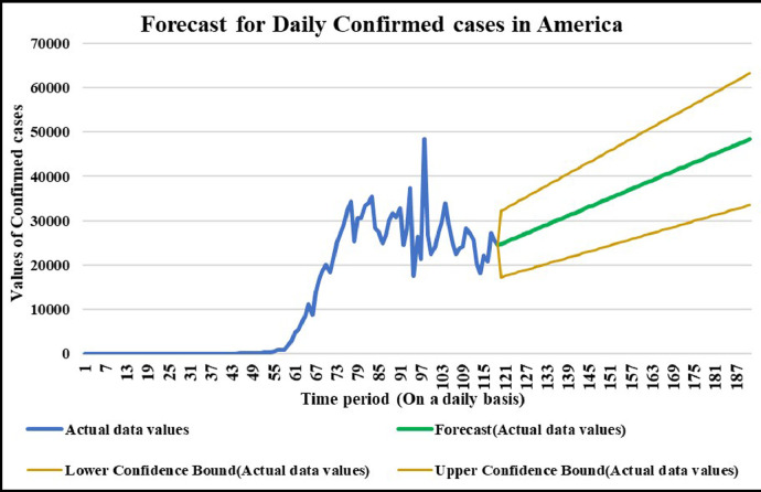
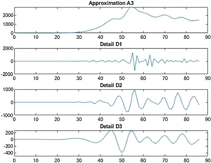
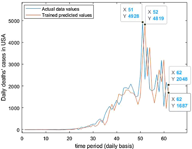
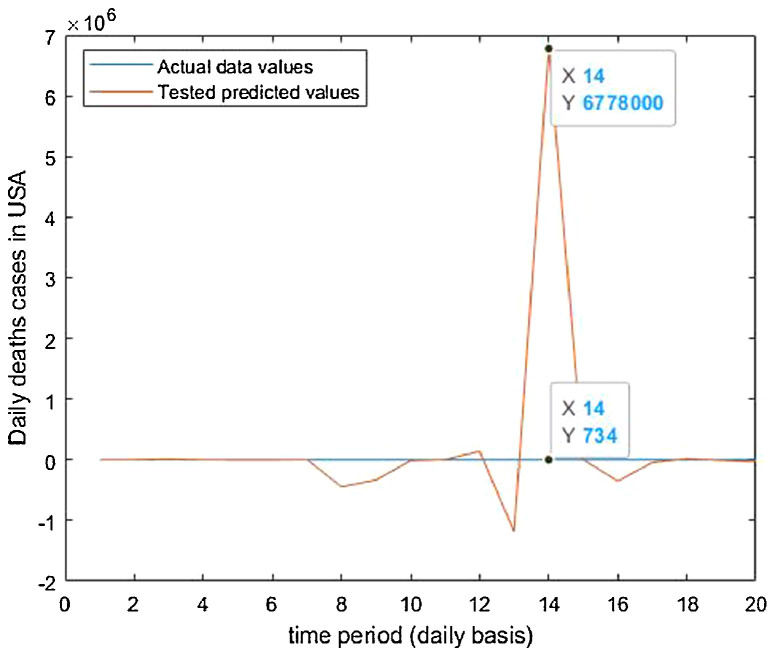
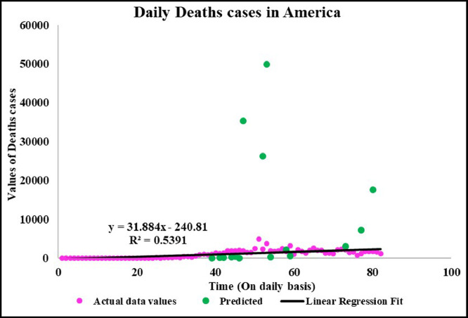
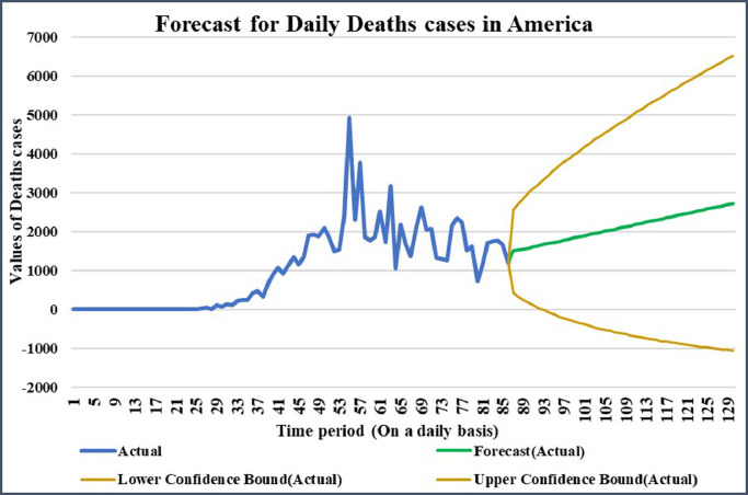
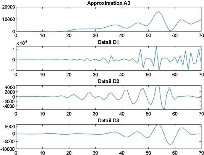
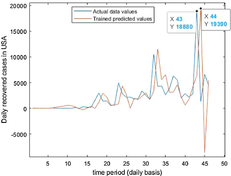
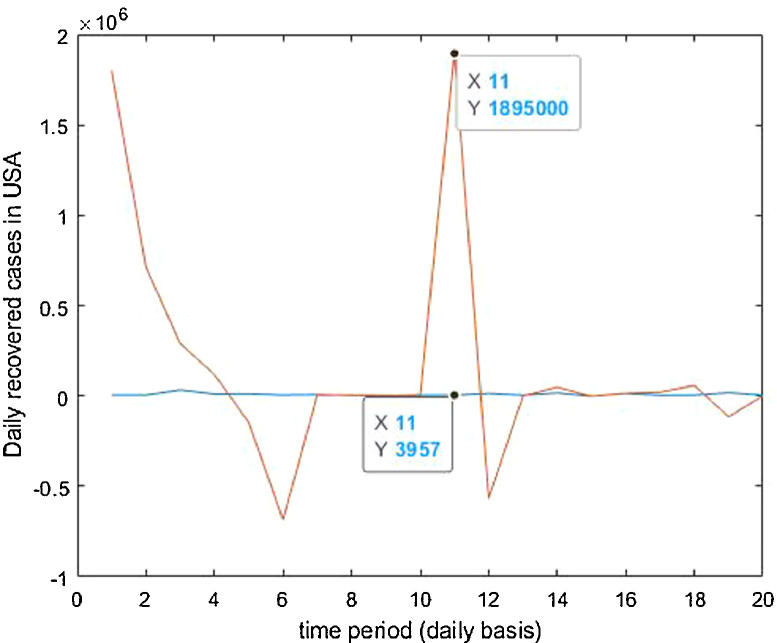
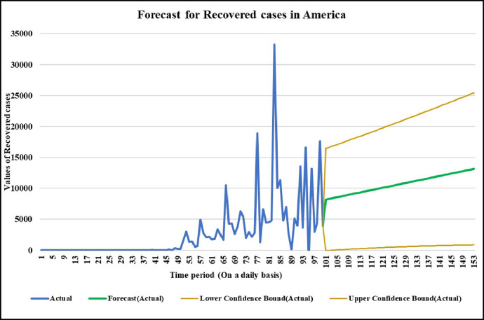
For the country of United States of America, the data has been analyzed under three main distinctions that are: Confirmed cases, Deaths’ cases and Recovery cases that are being recorded every day and provided through public bulletin from designated authorities as depicted through Fig. 37, Fig. 38, Fig. 39, Fig. 40, Fig. 41, Fig. 42, Fig. 43, Fig. 44, Fig. 45, Fig. 46, Fig. 47, Fig. 48, Fig. 49, Fig. 50, Fig. 51.

Fig. 37.

Wavelet decomposition of daily confirmed cases in USA.

Fig. 38.

Trained vs actual data values.

Fig. 39.

Tested vs actual data values.

Fig. 40.

Predicted vs actual data values with linear fit.

Fig. 41.

Forecasting longer time period with the past responses.

Fig. 42.

Wavelet decomposition of daily deaths cases in USA.

Fig. 43.

Trained vs actual data values.

Fig. 44.

Tested vs actual data values.

Fig. 45.

Predicted vs actual data values with linear fit.

Fig. 46.

Forecasting longer time period with the past responses.

Fig. 47.

Wavelet decomposition of daily recovered cases in USA.

Fig. 48.

Trained vs actual data values.

Fig. 49.

Tested vs actual data values.

Fig. 50.

Predicted vs actual data values with linear fit.

Fig. 51.

Forecasting longer time period with the past responses.

Case-1: Confirmed Cases in USA Daywise (Fig. 37, Fig. 38, Fig. 39, Fig. 40, Fig. 41 and 41 ).

Case-2: Deaths’ cases in USA daywise (Fig. 42, Fig. 43, Fig. 44, Fig. 45, Fig. 46 and 46 ).

Case-3: Recovered cases in USA Daywise (Fig. 47, Fig. 48, Fig. 49, Fig. 50, Fig. 51 and 51 ).

Conclusions

It is the need of the hour to model the factors of COVID-19 transmission to minimize its spread and the extent to which it can be harmful. Since, China is the first country to record and report such cases so it is in a way the breeding place of this epidemic. Thus, it is necessary to understand the scenario. Prevention measures should be followed at its best so that the virus does not communicate to more people and to stop its breeding further. The wavelet decomposition depicts the data filtered through high and low pass filters filtering the noise in the sense normalizing for further computations. The trained responses are plotted with the actual data values to compare the scenario of confirmed, deaths and recovered cases respectively. Simulations through time progression will aid in detailed study of virus structure dynamic evolution and perhaps indicate the emergence of randomness of the system. Then the regression fit for the predicted data depicts the goodness of fit of predicted data upon the actual data. Based on the simulations, the significance level (alpha) ranges from 0.10 to 0.67, MASE varying from 0.06 to 5.76, sMAPE ranges from 0.15% to 1.97%, MAE varies from 22.59 to 6024.76, RMSE shows a variation from 3.18 to 8360.29 & R² varying through 0.0018 to 0.7149. Clearly, in this study sMAPE and MASE have lower performance errors and therefore effective in forecast. Contribute towards better understanding of the scenario. Thus, the daily datasets pertaining to those of USA have a great variability as compared to China and India. Although, the spread has different timelines where India & America with the short time span have the greatest number of confirmed cases increasing uncontrollably at present. The forecast of 50–60 days ahead varying in every case helps to understand the clear picture of the pandemic spread and the manner in which the transmission rate may change in the following time periods in these three countries India, China and America.

The outcomes of this study can provide an efficient learning and understanding of the future spread estimation and to eradicate the panic and stigmas of the people worldwide towards COVID-19. Also, it may aid to improve clinical strategies against this pandemic. The best alternative left for the mankind at this moment is to follow preventive measures such as no direct human interaction, self-quarantine, keeping the living area hygienic and maintaining social distance.

Declaration of Competing Interest

The authors have no conflict of interest.

References

- 1.Anastassopoulou C., Russo L., Tsakris A., Siettos C. Data-based analysis, modelling and forecasting of the COVID-19 outbreak. PLoS ONE. 2020;15(3):1–21. doi: 10.1371/journal.pone.0230405. [DOI] [PMC free article] [PubMed] [Google Scholar]
- 2.Bailey N.T.J. 2 nd edition. Hafner; New York: 1975. The mathematical theory of lnfectious diseases. [Google Scholar]
- 3.Bhardwaj R., Bangia A. Complexity dynamics of meditating body. Indian J Ind Appl Math. 2016;7(2):106–116. [Google Scholar]
- 4.Bhardwaj R., Bangia A. Statistical time series analysis of dynamics of HIV. JNANABHA. 2018;(48):22–27. Special. [Google Scholar]
- 5.Bhardwaj R., Bangia A. Dynamic indicator for the prediction of atmospheric pollutants. Asian J Water Environ Pollut. 2019;16(4):39–50. [Google Scholar]
- 6.Bhardwaj R., Bangia A. Dynamical forensic inference for malware in iot-based wireless transmissions. In: Sharma K., Makino M., Shrivastava G., Agarwal B., editors. Forensic investigations and risk management in mobile and wireless communications. 2020. pp. 51–79. [Google Scholar]
- 7.Chakraborty T., Ghosh I. Real-time forecasts and risk assessment of novel coronavirus (COVID-19) cases: a data-driven analysis. Chaos Solitons Fractals. 2020;135:1–10. doi: 10.1016/j.chaos.2020.109850. 109850. [DOI] [PMC free article] [PubMed] [Google Scholar]
- 8.Fang Y., Nie Y., Penny M. Transmission dynamics of the COVID-19 outbreak and effectiveness of government interventions: a data-driven analysis. J Med Virol. 2020;92:645–659. doi: 10.1002/jmv.25750. [DOI] [PMC free article] [PubMed] [Google Scholar]
- 9.Huang N.E., Qiao F. A data driven time-dependent transmission rate for tracking an epidemic: a case study of 2019-nCoV. Sci Bull. 2020;65:425–427. doi: 10.1016/j.scib.2020.02.005. [DOI] [PMC free article] [PubMed] [Google Scholar]
- 10.Kucharski A.J., Russell T.W., Diamond C., Liu Y., Edmunds J., Funk S., Eggo R.M. Early dynamics of transmission and control of COVID-19: a mathematical modelling study. Lancet Infect Dis. 2020;20(5):553–558. doi: 10.1016/S1473-3099(20)30144-4. [DOI] [PMC free article] [PubMed] [Google Scholar]
- 11.Melin P., Monica J.C., Sánchez D., Castillo O. Analysis of spatial spread relationships of coronavirus (COVID-19) pandemic in the world using self organizing maps. Chaos Solitons Fractals. 2020;138 doi: 10.1016/j.chaos.2020.109917. 109917–109917. [DOI] [PMC free article] [PubMed] [Google Scholar]
- 12.Organization W.H . World Health Organization; 2020. World health organization (WHO). novel coronavirus - Japan (ex-China)https://www.who.int/csr/don/17-january-2020-novel-coronavirus-japan-ex-china/en/ cited January 20. Available. [Google Scholar]
- 13.Organization W.H. World health organization (WHO). Middle East respiratory syndrome coronavirus (MERS-CoV) - update: 2 December 2013. Available http://www.who.int/csr/don/2013_12_02/en/.
- 14.Organization W.H . 2020. World health organization (WHO)https://www.who.int/health-topics/coronavirus Coronavirus cited January 19. Available. [Google Scholar]
- 15.Pastor-Satorras R., Vespignani A. Epidemic spreading in scale-free networks. Phys Rev Lett. 2001;86(14):3200–3203. doi: 10.1103/PhysRevLett.86.3200. [DOI] [PubMed] [Google Scholar]
- 16.Prem K., Liu Y., Russell T.W., Kucharski A.J., Eggo R.M., Davies N. The effect of control strategies to reduce social mixing on outcomes of the COVID-19 epidemic in Wuhan, China: a modelling study. The Lancet Public Health. 2020;5(5):e261–e270. doi: 10.1016/S2468-2667(20)30073-6. [DOI] [PMC free article] [PubMed] [Google Scholar]
- 17.Roda W.C., Varughese M.B., Han D., Li M.Y. Why is it difficult to accurately predict the COVID-19 epidemic. Infect Dis Model. 2020;5:271–281. doi: 10.1016/j.idm.2020.03.001. [DOI] [PMC free article] [PubMed] [Google Scholar]
- 18.Rustam F., Reshi A.A., Mehmood A., Ullah S., On B.-.W., Aslam W., Choi G.S. COVID-19 Future forecasting using supervised machine learning models. IEEE Access. 2020;8:101489–101499. [Google Scholar]
- 19.Salgotra R., Gandomi M., Gandomi A.H. Time series analysis and forecast of the COVID-19 pandemic in India using genetic programming. Chaos Solitons Fractals. 2020;138:1–15. doi: 10.1016/j.chaos.2020.109945. 109945. [DOI] [PMC free article] [PubMed] [Google Scholar]
- 20.Santosh K.C. AI-Driven tools for coronavirus outbreak: need of active learning and cross-population train/test models on multitudinal/multimodal data. J Med Syst. 2020;44:1–5. doi: 10.1007/s10916-020-01562-1. [DOI] [PMC free article] [PubMed] [Google Scholar]
- 21.Wu C.-.Y., Jan J.-.T., Ma S.-.H., Kuo C.-.J., Juan H.-.F., Cheng Y.-.S.E. Small molecules targeting severe acute respiratory syndrome human coronavirus. Proc Natl Acad Sci. 2004;101:10012–10017. doi: 10.1073/pnas.0403596101. [DOI] [PMC free article] [PubMed] [Google Scholar]
- 22.Wu J.T., Leung K., Leung G.M. Nowcasting and forecasting the potential domestic and international spread of the 2019-nCoV outbreak originating in Wuhan, China: a modelling study. Lancet. 2020;395:689–697. doi: 10.1016/S0140-6736(20)30260-9. [DOI] [PMC free article] [PubMed] [Google Scholar]
- 23.Zhong L., Mu L., Li J., Wang J., Yin Z., Liu D. Early prediction of the 2019 novel coronavirus outbreak in the mainland China based on simple mathematical model. IEEE Access. 2020;8:51761–51769. doi: 10.1109/ACCESS.2020.2979599. [DOI] [PMC free article] [PubMed] [Google Scholar]
- 24.Zhou P., Yang X.L., Wang X.G., Hu B., Zhang L., Zhang W. A pneumonia outbreak associated with a new coronavirus of probable bat origin. Nature. 2020;579:270–273. doi: 10.1038/s41586-020-2012-7. [DOI] [PMC free article] [PubMed] [Google Scholar]