Abstract
The recent spread of COVID-19 has led to the worst economic crisis since the 1930s. To boost demand after the crisis, direct monetary transfers to households are being discussed. Using novel microdata from the Eurosystem Household Finance and Consumption Survey (HFCS), we study how much of such a transfer households would actually spend. We do so by exploiting the unique opportunity that the new wave of the survey included an experimental question to calculate the marginal propensity to consume from hypothetical windfall gains. Our results show that households on average spend between about 33% (the Netherlands) and 57% (Lithuania) of such a transfer. In all countries, answers are clustered at spending nothing, spending 50% and spending everything. Marginal propensities to consume decrease with income but are not as clearly related to wealth.
Keywords: Survey data, Helicopter money, Household finance, Monetary policy
Highlights
-
•
We discuss helicopter money as an option to boost demand after the COVID-19 crisis.
-
•
Marginal propensity to consume across euro area countries is between 33% and 57%.
-
•
Marginal propensity to consume decreases with income but is unrelated to wealth.
-
•
Helicopter money would lead to heterogeneous effects across and within countries.
-
•
Lump-sum transfers might be preferable to inequality-preserving transfers.
1. Introduction
In recent months helicopter money has been widely discussed as a potential tool to boost the economy once the COVID-19 health crisis is under control. Several blog posts and new working papers discuss the issue.1 Nevertheless, cross country empirical evidence is still scarce on how helicopter money is actually spent.
The literature on the marginal propensity to consume (MPC) is, theoretical as well as empirical, among the largest and oldest fields in economics. Japelli and Pistaferri (2010) provide an excellent overview. In a more recent contribution, Japelli and Pistaferri (2014) base their analysis on a hypothetical question in an Italian household survey to examine the marginal propensity to consume (MPC) out of windfall gains. More recently, the contributions of De Haan and van Rooij (2019) and Djuric and Neugart (2019) analyze similar survey questions for the Netherlands and Germany.
Japelli and Pistaferri (2014) documented an average MPC of about 48% for Italy, Djuric and Neugart (2019) one of about 40% for Germany, and De Haan and van Rooij (2019) one of 30% for the Netherlands. Furthermore, Christelis et al. (2019) look specifically at the symmetry of a positive versus a negative income shock reporting an MPC of about 25% for Dutch households. Another strand of the literature investigates the effect of income shocks on neighbors’ behavior as for example in Kuhn et al. (2011) who find a positive effect on car consumption of neighbors of households winning a car.
However, the MPC resulting from windfall gains has to the best of our knowledge not been examined on the basis of internationally comparable microdata for a large set of countries including the whole balance sheet of households. Note, that using a question on hypothetical windfall gains instead of actual gains allows to include all households (represented by the sample) in the analysis, while analyses of actual gains are often restricted to small subsets of the population. We contribute to the literature by examining the MPC out of a windfall gain for a set of 17 European countries (including all euro area countries but Finland, Spain and Estonia) based on a harmonized survey question within the main European survey to analyze household finances. We estimate the average MPC across countries and the full distribution of income and wealth. We find heterogeneity across country means as well as strong differences in distributional patterns with regard to extreme saving or spending behavior. While the average MPC clearly decreases with income, it shows no correlation with wealth. We conclude that a standardized monetary intervention via helicopter money in the euro area would lead to very heterogeneous effects across different countries, but also within countries across households.
2. Data
The data come from the third wave of the Eurosystem HFCS and was published in April 2020.2 While the survey was conducted in 22 countries, only 17 countries included the question on a windfall gain. This question is ideal for analyzing the topical issue of helicopter money. We use individual household-level data for Austria (AT), Belgium (BE), Cyprus (CY), Germany (DE), France (FR), Greece (GR), Croatia (HR), Ireland (IE), Italy (IT), Lithuania (LT), Luxembourg (LU), Latvia (LV), Malta (MT), the Netherlands (NL), Portugal (PT), Slovakia (SK) and Slovenia (SI), altogether comprising 58,515 observations without any missing information.3 The unique feature of this survey we use is the experimental question on helicopter money, which was implemented as a hypothetical windfall gain from a lottery win of an amount equal to the net income a household receives in one month. The data also contain standard socioeconomic demographic characteristics as well as detailed information on the balance sheets of households.
Similar to Jappelli and Pistaferri (2014), our main variable of interest is the hypothetical question on the windfall gain a household receives. The question posed to households is
Imagine you unexpectedly receive money from a lottery, equal to the amount of income your household receives in a month. What percent would you spend over the next 12 months on goods and services, as opposed to any amount you would save for later or use to repay loans?
Following the existing literature, we estimate the marginal propensity to consume out of such a windfall gain. In particular, we are interested in its distribution across household incomes as well as across countries, because both are crucial to designing a potential helicopter money policy and evaluating its potential impact. On top of that, our survey allows for an assessment of the MPC across the distribution of net wealth as well. Table 1 shows descriptions of all variables we use in the analysis. Summary statistics of the surveys and main variables used in our empirical analysis are presented in Table 2.
Table 1.
Description of variables.
| Name | Explanation | Definition |
|---|---|---|
| hiz0400a | Spending | How much of an lottery gain of one month households income is spent over the next 12 months on goods and services |
| dn3001 | Net wealth | Total household assets excluding public and occupational pension wealth minus total outstanding household’s liabilities (excluding public pensions) |
| di2000 | Gross income | Total gross annual household income aggregate |
| dh0001 | Household size | Number of household members, all household members included |
| dhageh1b | Age brackets | Age of the RP (UN/Canberra definition used in the ECB-HFCS statistical output) in brackets: 16–19, 20–24, 25–29, 30–34, 35–39, 40–44, 45–49, 50–54, 55–59, 60–64, 65–69, 70–74, 75–79, 80–84, 85 and older |
| dhaged65plus | Old age | Household members aged 65 or more |
HFCS 2017.
Table 2.
Descriptive statistics.
| Country | Non-missing obs. | All observations | % of missing MPC | Average MPC (%) | Net wealth |
Gross income |
||
|---|---|---|---|---|---|---|---|---|
| Mean | Median | Mean | Median | |||||
| Austria | 3,072 | 3,072 | 0.0 | 46.6 | 250.3 | 82.6 | 50.4 | 41.2 |
| (0.8) | (22.3) | (3.9) | (1.4) | (0.5) | ||||
| Belgium | 2,275 | 2,329 | 2.3 | 42.0 | 366.2 | 212.2 | 56.4 | 43.5 |
| (1.1) | (21.4) | (9.4) | (1.2) | (1.0) | ||||
| Cyprus | 1,303 | 1,303 | 0.0 | 43.7 | 499.7 | 195.4 | 32.9 | 25.3 |
| (1.6) | (58.6) | (15.4) | (0.9) | (1.1) | ||||
| Germany | 4,940 | 4,942 | 0.0 | 51.3 | 232.8 | 70.7 | 53.1 | 40.1 |
| (0.8) | (8.7) | (3.4) | (0.9) | (0.7) | ||||
| France | 13,685 | 13,685 | 0.0 | 41.8 | 242.0 | 117.6 | 40.5 | 32.3 |
| (0.5) | (5.3) | (5.4) | (0.4) | (0.5) | ||||
| Greece | 2,964 | 3,007 | 1.4 | 56.8 | 93.9 | 60.0 | 22.5 | 19.0 |
| (1.0) | (3.8) | (2.5) | (0.4) | (0.4) | ||||
| Croatia | 1,335 | 1,357 | 1.6 | 55.7 | 106.6 | 61.4 | 12.2 | 8.4 |
| (1.2) | (8.5) | (3.3) | (0.5) | (0.4) | ||||
| Ireland | 4,517 | 4,793 | 5.8 | 52.8 | 367.8 | 184.9 | 65.2 | 48.0 |
| (0.9) | (11.3) | (6.1) | (1.5) | (0.7) | ||||
| Italy | 7,420 | 7,420 | 0.0 | 48.1 | 214.3 | 132.1 | 33.8 | 24.6 |
| (0.7) | (5.0) | (3.0) | (0.5) | (0.3) | ||||
| Lithuania | 1,444 | 1,664 | 13.2 | 57.3 | 84.3 | 45.8 | 10.8 | 7.1 |
| (1.7) | (5.8) | (2.0) | (0.6) | (0.3) | ||||
| Luxembourg | 1,616 | 1,616 | 0.0 | 37.1 | 897.9 | 498.0 | 93.1 | 71.0 |
| (1.0) | (45.4) | (23.2) | (1.9) | (1.9) | ||||
| Latvia | 1,196 | 1,249 | 4.2 | 51.3 | 43.0 | 20.5 | 14.3 | 10.2 |
| (1.8) | (2.7) | (1.5) | (0.3) | (0.3) | ||||
| Malta | 1,004 | 1,004 | 0.0 | 48.8 | 400.7 | 236.0 | 31.2 | 25.4 |
| (0.9) | (29.3) | (6.4) | (1.0) | (0.9) | ||||
| Netherlands | 1,735 | 2,556 | 32.1 | 32.9 | 186.0 | 67.3 | 54.8 | 44.8 |
| (0.7) | (9.9) | (4.1) | (1.0) | (0.8) | ||||
| Portugal | 5,816 | 5,924 | 1.8 | 33.2 | 162.3 | 74.8 | 24.6 | 17.6 |
| (0.7) | (7.2) | (2.2) | (0.6) | (0.3) | ||||
| Slovenia | 2,014 | 2,014 | 0.0 | 48.7 | 144.3 | 91.5 | 22.3 | 16.4 |
| (1.2) | (7.4) | (3.1) | (0.5) | (0.5) | ||||
| Slovakia | 2,179 | 2,179 | 0.0 | 54.0 | 103.5 | 70.3 | 20.3 | 16.0 |
| (1.1) | (5.0) | (2.7) | (0.8) | (0.4) | ||||
| All | 58,515 | 60,114 | 2.7 | 46.9 | 224.5 | 94.7 | 43.0 | 31.6 |
Note: Wealth and yearly household income shown in EUR thousands based on all observations. Standard errors are shown in parentheses. Standard errors are based on 500 replicate weights taking into account the complex survey design and multiple imputations. Multiple imputations are available for all countries in the case of income and wealth. Missing MPCs are excluded for those countries which do not impute them.
HFCS 2017.
3. Methods
We use straightforward tools to describe the empirical results of the question at hand. Note, however, that we use both complex survey population weights and multiple imputations for all statistics shown. While the multiple imputations would not be very important for the experimental question alone, they are crucial for obtaining the correct correlations with income and wealth. We show the full distribution of answers to the experimental question using a detailed histogram. We calculate the average marginal propensity to consume across all countries. And we use two tools to describe large datasets while keeping the micro perspective alive:
First, we use locally weighted non-parametric linear regressions (loess) to estimate the share of households providing an answer at the end of the spectrum by saying that they spend nothing (MPC 0) or all (MPC 1) across the full distribution of gross income4 (using the cumulative distribution function).
Second, we use binned scatter plots where average MPCs of bins including an equal number of households (weighted observations) are calculated across gross income and net wealth. In a second step we also use binned scatter plots of the same variables, but residualized. Thus, by using linear regression and the Frisch–Waugh–Lovell theorem variation explainable by a set of control variables is filtered out before plotting.
4. Results
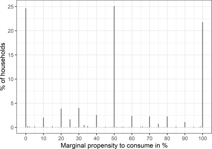
Fig. 1 shows the full range of answers to the question on how much of the windfall gain would be spent. One can clearly see that the answers are clustered at three points: saving all (MPC 0), saving/spending half (MPC 0.5) and spending all (MPC 1). This finding holds also at the country level for all countries, however in varying degrees. It also ties in with the findings of the literature discussed.
Fig. 1.
Distribution of marginal propensity to consume. Note: Pooled data.
HFCS 2017.
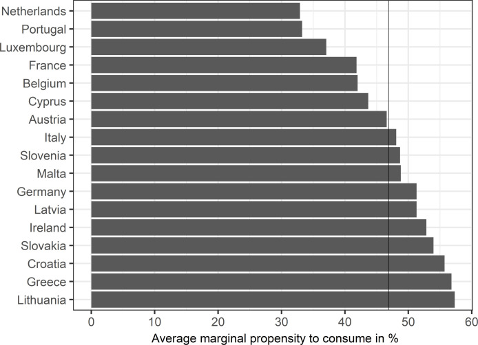
Fig. 2 shows the average MPC across all countries. The results of Japelli and Pistaferri (2014) for Italy and De Haan and van Rooij (2019) for the Netherlands are almost replicated. Only compared to Djuric and Neugart (2019), who found an average MPC of about 40% for Germany, do we find a much higher MPC (of about 51%).
Fig. 2.
Average marginal propensity to consume across countries. Note: Line shows the average marginal propensity to consume for the pooled data.
HFCS 2017.
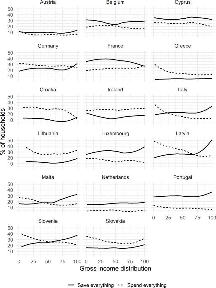
Fig. 3 shows the results of locally weighted linear regressions (loess) to smooth the share of answers at the end of the spectrum – spending all and saving all – across the gross income distributions of all countries. It illustrates that behind the average MPC there exists a lot of cross-country heterogeneity in terms of MPCs across the gross income distributions. In some countries the share of those who save everything is higher across the full distribution of gross income. In others the share of those who spend everything dominates. In some countries the correlation with income is much stronger than in others. All these patterns illustrate that overall the effects of euro area-wide helicopter money might be rather heterogeneous not only on average across countries but also in terms of different patterns across and within countries.
Fig. 3.
Share of households saving or spending everything (MPC 0 and MPC 1). Note: Gross Income distributions are constructed via cdfs at the country level.
HFCS 2017.
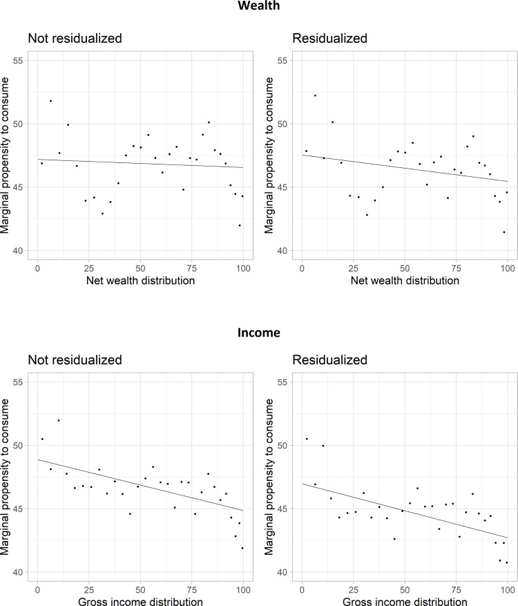
Fig. 4 shows four binned scatter plots. In all of them each dot represents about 4.2 million households and is calculated based on about 1930 observations (on average). All figures show average MPCs across the income and wealth distributions of the pooled data. The residualized plots control for country dummies,5 households size, age of the reference person based on 15 categories and a dummy variable indicating that at least one person living in the household is 65 years or older, and wealth (in the case of income) or income (in the case of wealth). The data offer the unique opportunity to analyze average MPC together with wealth. One can clearly see that there is hardly any correlation between households net wealth and their MPC. By contrast, there is clearly a negative correlation between MPC and income. One reason for this difference might be that income is immediately available for spending. Conversely, a large part of household wealth such as housing, cars or other real assets but also part of the financial assets is not directly available for spending but would need to be liquidated or used as a collateral first.
Fig. 4.
Average marginal propensity to consume across income and wealth. Note: The figures show binned scatter plots of the pooled data. Each dot represents about 4.2 million households and is calculated based on about 1930 observations (on average). The net wealth and gross income distributions are cdfs constructed on the pooled data. Residualized plots control for country dummies, household size, age of the reference person based on 15 categories and a dummy variable indicating that at least one person living in the household is 65 years or older, as well as income in the case of wealth and wealth in the case of income.
HFCS 2017.
5. Concluding remarks
Using microdata comparable across 17 european countries, we find that the average marginal propensities to consume (MPCs) vary considerably across countries. The MPC is lowest – at about 33% – in the Netherlands and Portugal and highest – at about 57% – in Greece and Lithuania. Patterns behind average MPCs differ strongly across countries. MPCs are negatively correlated with gross income but the relationship to wealth is less clear.
Based on the empirical evidence at hand we conclude that helicopter money – if applied equally across euro area countries – would likely have very heterogeneous effects across different countries. But also within countries, the effects would be related to the spending patterns along the income distribution, with a relatively stronger impact on goods and services consumed by lower income households exceeding their proportion of general spending/income.
Given the higher MPC in lower income groups, one policy conclusion could be that a lump sum transfer is preferable to an inequality-preserving amount proportional to net income.
Footnotes
See for example: https://voxeu.org/article/fight-covid-pandemic-policymakers-must-move-fast-and-break-taboos; https://www.moneyandbanking.com/commentary/2020/5/10/helicopters-to-the-rescue; https://cepr.org/active/publications/discussion_papers/dp.php?dpno=14734 (all accessed 08.07.2020)..
Detailed information about the survey can be found at https://www.ecb.europa.eu/pub/economic-research/research-networks/html/researcher_hfcn.en.html.
All HFCS data is multiply imputed five times. However, not all countries included the experimental question into their list of variables to be imputed. That is why for calculations of the MPC we can only use 58,515 observations out of the total 60,114 for all countries (see Table 1). We use Rubin’s Rule for all calculations.
We use the cdf of gross income for several reasons: First, net income is not available in the HFCS. Second, because of potential measurement error we only use the ranking of households and not their actual income values. The ranking should also be highly correlated with the ranking according to net income.
Country-level fixed effects should control for differences in the levels of income or wealth due to institutional differences or differences in national price levels.
References
- Christelis D., Georgarakos D., Jappelli T., Pistaferri L., van Rooij M. Asymmetric consumption effects of transitory income shocks. Econ. J. 2019;129(622):2322–2341. [Google Scholar]
- De Haan J., van Rooij M. Would helicopter money be spent? New evidence for the Netherlands. Appl. Econ. 2019;51(58):6171–6189. [Google Scholar]
- Djuric U., Neugart M. Helicopter money: Survey evidence on expectation formation and consumption behavior. Oxf. Econ. Pap. 2019 doi: 10.1093/oep/gpz062. gpz062. [DOI] [Google Scholar]
- Japelli T., Pistaferri L. The consumption response to income changes. Annu. Rev. Econ. 2010;2(1):479–506. [Google Scholar]
- Japelli T., Pistaferri L. Fiscal policy and MPC heterogeneity. Am. Econ. J.: Macroecon. 2014;6(4):107–136. [Google Scholar]
- Kuhn P., Kooreman P., Soetevent A., Kapteyn A. The effects of lottery prizes on winners and their neighbors: Evidence from the dutch postcode lottery. Amer. Econ. Rev. 2011;101(5):2226–2247. [Google Scholar]


