Threshold dynamics of a time-delayed epidemic model for continuous imperfect-vaccine with a generalized nonmonotone incidence rate

Abstract

In this paper, we study the dynamics of an infectious disease in the presence of a continuous-imperfect vaccine and latent period. We consider a general incidence rate function with a non-monotonicity property to interpret the psychological effect in the susceptible population. After we propose the model, we provide the well-posedness property and calculate the effective reproduction number ${\mathcal{R}}_E$. Then, we obtain the threshold dynamics of the system with respect to ${\mathcal{R}}_E$ by studying the global stability of the disease-free equilibrium when ${\mathcal{R}}_E<1$ and the system persistence when ${\mathcal{R}}_E>1$. For the endemic equilibrium, we use the semi-discretization method to analyze its linear stability. Then, we discuss the critical vaccination coverage rate that is required to eliminate the disease. Numerical simulations are provided to implement a case study regarding data of influenza patients, study the local and global sensitivity of ${\mathcal{R}}_E<1$, construct approximate stability charts for the endemic equilibrium over different parameter spaces and explore the sensitivity of the proposed model solutions.

Introduction

In 1979, Cooke introduced a “time delay” to represent the disease incubation period in studying the spread of an infectious disease transmitted by a vector in [1]. Since then, many authors have incorporated time delays in epidemic models in different scenarios, such as vaccination period [2], asymptomatic carriage period [3], immune period [4] and incubation period or latent period [3–7]. More precisely, in [3], a disease transmission model with two delays in incubation and asymptomatic carriage periods is investigated. In [4], the authors study an SEIRS epidemic model with constant latent and immune periods. In [5], a latent period and relapse are considered in a general mathematical model for disease transmission. In [7], the authors studied a time-delayed SIR model with nonlinear incidence rate and Holling functional type II treatment rate for epidemic transmission. Also, many authors studied time-delayed epidemic models with vaccination [8–11]. For example, the authors in [9] study a vaccination model with a time delay to represent the time that an unaware susceptible individual takes to become aware of the infection. Due to the inherent complexity of epidemiological transmission, other works studied epidemic complex network models. For example, in [12], the authors studied a semi-random epidemic network and discussed the relationship between its topological structure and the optimal control of the epidemic. In [13], the authors used the concept of epidemiology to analyze data from real computer virus epidemics by using complex network models. They studied an SIS model on scale-free graphs by largescale simulations and analytical methods.

Vaccines are considered to be one of the most significant medical means of disease control and prevention [14]. They have played a major role in the spread and eradication of many infectious diseases, such as smallpox, or partially, like measles. Many authors in the literature have studied the dynamics of epidemics models with different types of vaccination schedules [15–19]. For instance, in [16], an SIR model with a generalized incidence under preventive vaccination and treatment controls is proposed. In [20], the authors developed an SIVS epidemic model with degree-related transmission rates and imperfect vaccination on scale-free networks. In [17], the authors establish two SVIR models: one with continuous vaccination strategy and another one with pulse vaccination strategy. An epidemic model to study the potential impact of a SARS vaccine when it is imperfect is proposed in [18]. The dynamics of cholera epidemics with impulsive vaccination is studied in [15].

To incorporate the effect of behavioral changes on the disease spreading dynamics, the authors in [21] introduce a nonlinear incidence rate of the form

$$\begin{array}{c}\hfill Sg(I)=\frac{\beta S{I}^{q_1}}{1+d{I}^{q_2}}\end{array}$$ 1

where S and I represent the numbers of susceptible and infectious individuals, respectively, $\beta$ is the probability of transmission per contact per unit time, and the constant $q_1$ is positive while the constants $q_2,d$ are nonnegative. Here, the constant d measures the inhibitory effect. In (1), $\beta I^{q_1}$ measures the infection force of the disease and $1/(1+d{I}^{q_2})$ represents the inhibition effect from the behavioral change of the susceptible individuals when the number of infectious individuals increase [22]. It also can be used to describe the crowding effect of infectious individuals [23]. There are three types of incidence functions $g(I)=\beta I^{q_1}/(1+d{I}^{q_2})$ based on the values of $q_1$ and $q_2$ [22, 24]: (i) unbounded incidence function: $q_1>q_2$; (ii) saturated incidence function: $q_1=q_2$; and (iii) nonmonotone incidence function: $q_1<q_2$. In the literature, these types have been used in different scenarios. For example, the authors in [22] consider a nonmonotone incidence rate to represent the psychological effect with $q_1=1$ and $q_2=2$. In [23], a saturated incidence rate is considered with $q_1=q_2=2$. For more details and examples, we refer the reader to [24] and references within. In this paper, we consider a general form of an nonmonotone infection force function g(I), in the sense that g(I) is increasing when the population of infectious I is small and decreasing when I is large. From a biological point of view, this can be interpreted as the “psychological effect”, that is, when a disease is spreading among a population and the number of infective individuals becomes large, the behavior of the population may tend toward reducing the number of contacts among individuals per unit time [22].

In the real world, the latent period may vary from days, as in influenza A H1N1 [25], to years, as in AIDS [26]. The latent period has a profound effect on the generation time, which is defined as the time period between a case becoming infected and its subsequent infection of another case [27]. Thus, the latent period has an influence on the epidemic growth [28]. The purpose of the work is to investigate the dynamical behavior of a time-delayed SEIR model with continuous imperfect-vaccine and discuss the effect of the latent period on the epidemic. The paper is organized as follows. In the next section, we present the mathematical model and the study its well-posedness. Then, in Sect. 3, we calculate the effective reproduction number ${\mathcal{R}}_E$. In Sect. 4, we use various methods, such as the Lyapunov functional technique and the method of fluctuations, to establish the global stability of the disease-free equilibrium when ${\mathcal{R}}_E<1$. Then, in Sect. 5, we study the system persistence when ${\mathcal{R}}_E>1$. Moreover, we use the semi-discretization method of order one to study the local stability of endemic equilibrium. In Sect. 6, we discuss the critical vaccination coverage that is required to eliminate the disease. In Sect. 7, we consider an application to influenza transmission. Numerically, we also study the local and global sensitivities of ${\mathcal{R}}_E$, discuss the stability of the endemic equilibrium and examine the sensitivity of model solutions. Finally, we discuss our results in Sect. 8.

Mathematical model and the well-posedness property

Motivated by [29], we let N(t) be the total population at time t and divide it into five classes: S(t) is the susceptible population, V(t) is the population of vaccinated individuals, E(t) is the population of individuals who are infected but not yet infectious (exposed class), I(t) is the infected population and R(t) is the recovered population. We assume there is a recruitment rate into the population and the natural death rate is the same for all the compartments. We make the following assumptions to describe the interaction among the five classes:

• When the susceptible individuals receive a vaccine, they move from class S to V. On the other side, the infected individuals in S move to the exposed class E with transmission rate $\beta$ and remain there for a certain latent period $\tau$ (see e.g., [30]);

• The vaccine is not perfect, in the sense that, the individuals in V are not on a fully protective level. Consequently, when the vaccinated individuals become infected, they move into E for $\tau$ period with a reduced transmission rate $\xi \beta$, where $\xi \in [0,1]$ is the reduction coefficient [30]. When individuals gain immunity, they move into the class R [17];

• After the latent period $\tau$, infected individuals become infectious and move from E to I. Then when they recover, they move to R. Individuals in R may lose immunity at rate $\alpha$ and become susceptible again, that is, they move to the class S (i.e., the vaccine is continuous).

These assumptions lead to the following system of delay differential equations:

$$\begin{array}{c}\hfill \begin{array}{cc}\hfill \frac{\mathrm{d}S}{\mathrm{d}t}& =\mathrm{\Lambda }-\frac{\beta S(t)I(t)}{f(I(t))}-\left(\mu ,+,\psi \right)S(t)+\alpha R(t),\hfill \\ \hfill \frac{\mathrm{d}V}{\mathrm{d}t}& =\psi S(t)-\frac{\xi \beta V(t)I(t)}{f(I(t))}-(\mu +\eta )V(t),\hfill \\ \hfill \frac{\mathrm{d}E}{\mathrm{d}t}& =\frac{\beta (S(t)+\xi V(t))I(t)}{f(I(t))}\hfill \\ \hfill & -\frac{\beta (S(t-\tau )+\xi V(t-\tau ))I(t-\tau )}{f(I(t-\tau ))}{\mathrm{e}}^{-\tau \mu }\hfill \\ \hfill & -\mu E(t),\hfill \\ \hfill \frac{\mathrm{d}I}{\mathrm{d}t}& =\frac{\beta (S(t-\tau )+\xi V(t-\tau ))I(t-\tau )}{f(I(t-\tau ))}{\mathrm{e}}^{-\mu \tau }\hfill \\ \hfill & -(\mu +\gamma )I(t),\hfill \\ \hfill \frac{\mathrm{d}R}{\mathrm{d}t}& =\eta V(t)+\gamma I(t)-(\mu +\alpha )R(t).\hfill \end{array}\end{array}$$ 2

The term ${\mathrm{e}}^{-\mu \tau }$ represents the probability for individuals to survive the latent period $[t-\tau ,t]$, see e.g., [3]. The population flux among the five compartments is given in Fig. 1 and a description of the parameters is given in Table 1.

Fig. 1.

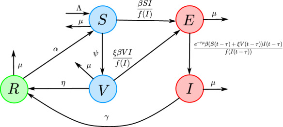
The flow diagram for system (2)

Table 1.

Parameter description of the system (2)

Parameter	Description
$\mathrm{\Lambda }$	Recruitment rate of susceptible humans
$\beta$	Effective contact rate
$\psi$	Vaccination coverage rate
$\mu$	Natural mortality rate
$\alpha$	Loosing immunity
$\xi$	The vaccine efficacy is $ϵ=1-\xi$
$1/\eta$	The immunity development period
$\tau$	Latent period
$\gamma$	Recovery rate

Denote the infection force function by $\beta I/f(I)$. Following [16, 31], we assume that the infection force function decreases when the number of infectious individuals increases since the individuals tend to reduce the number of contacts among them per unit time when they are under intervention policies. Consequently, we consider the following assumptions:

Here, $\zeta$ is the critical level of invectives, that is, the incidence rate is increasing when $I\in (0,\zeta ]$ and it is decreasing when $I>\zeta$. Notice that the nonlinear incidence rate has the form $\frac{\beta (S+\xi V)I}{f(I)}$.

Consider the Banach space $\mathcal{C}:=C([-\tau ,0),{\mathbb{R}}^5)$ with the maximum norm

$$\begin{array}{cc}& ∥\varphi ∥=\sum _{i=1}^5\left(\underset{\theta \in \left[-\tau ,0\right]}{max}\left|{\varphi }_i(\theta )\right|\right),\hfill \\ \hfill & \forall \varphi =({\varphi }_1,{\varphi }_2,{\varphi }_3,{\varphi }_4,{\varphi }_5)\in \mathcal{C}.\hfill \end{array}$$

Then ${\mathcal{C}}^{+}:=C([-\tau ,0],{\mathbb{R}}_{+}^5)$ is a normal cone of $\mathcal{C}$ and the interior of $\mathcal{C}$ is not empty. Let $r>0$ and $u=(u_1,u_2,u_3,u_4,u_5):[-\tau ,r)\to {\mathbb{R}}^5$ be a continuous function. For $t\ge 0$, define $u_t\in \mathcal{C}$ by $u_t(\theta )=(u_1(t+\theta ),u_2(t+\theta ),u_3(t+\theta ),u_4(t+\theta ),u_5(t+\theta ))$ for all $\theta \in [-\tau ,0]$.

The initial data set for system (2) is in form:

$$\begin{array}{cc}\hfill \mathbb{X}=& \left\{\varphi ,\in ,{\mathcal{C}}^{+},:,{\varphi }_3,(0)\right)\hfill \\ \hfill & \left(=,\underset{-\tau }{\overset{0}{\int }},\left(\frac{\beta {\varphi }_3(s)({\varphi }_1(s)+\xi {\varphi }_4(s))}{f\left({\varphi }_3(s)\right)}{\mathrm{e}}^{\mu s}\right)\mathrm{d}s\right\}\hfill \end{array}$$

where the form for ${\varphi }_3(0)$ follows from the implicit solution of E(t) in system (2) which has form:

$$\begin{array}{c}\hfill E(t)=\underset{t-\tau }{\overset{t}{\int }}\left(\frac{\beta I(\theta )(S(\theta )+\xi V(\theta ))}{f\left(I(\theta )\right)}{\mathrm{e}}^{-\mu (t-\theta )}\right)\mathrm{d}\theta .\end{array}$$ 3

The following theorem shows the nonnegativity and boundedness of system (2).

Theorem 2.1

Let $\varphi \in \mathbb{X}$. Then, system (2) has an ultimately bounded unique non-negative solution (S(t), V(t) , E(t), I(t), R(t)) for $t\ge 0$ in $\mathcal{C}$. Furthermore, the region

$$\begin{array}{cc}\hfill \mathrm{\Gamma }=& \left\{\left(S(t),V(t),E(t),I(t),R(t)\right),\in ,{\mathbb{R}}_{+}^5,:\right)\hfill \\ \hfill & \left(S,(t),+,V,(t),+,E,(t),+,I,(t),+,R,(t),=,\frac{\mathrm{\Lambda }}{\mu }\right\}\hfill \end{array}$$

is a positive invariant set and globally attractive set for (2).

Proof

For any $\varphi \in \mathbb{X}$, we define $G(\varphi )=(G_1(\varphi ),G_2(\varphi )$$,G_3(\varphi ),G_4(\varphi ),G_5{(\varphi ))}^T$, where

$$\begin{array}{cc}\hfill G_1(\varphi )=& \mathrm{\Lambda }-\beta \frac{{\varphi }_1(0){\varphi }_4(0)}{f({\varphi }_4(0))}\hfill \\ \hfill & -(\mu +\psi ){\varphi }_1(0)+\alpha {\varphi }_5(0),\hfill \\ \hfill G_2(\varphi )=& \psi {\varphi }_1(0)-\beta \xi \frac{{\varphi }_2(0){\varphi }_4(0)}{f({\varphi }_4(0))}-(\mu +\eta ){\varphi }_2(0),\hfill \\ \hfill G_3(\varphi )=& \beta \frac{\left({\varphi }_1(0)+\xi {\varphi }_2(0)\right){\varphi }_4(0)}{f({\varphi }_4(0))}\hfill \\ \hfill & -\beta \frac{\left({\varphi }_1(-\tau )+\xi {\varphi }_2(-\tau )\right){\varphi }_4(-\tau )}{f({\varphi }_4(-\tau ))}{\mathrm{e}}^{-\mu \tau }\hfill \\ \hfill & -\mu {\varphi }_3(0),\hfill \\ \hfill G_4(\varphi )=& \beta \frac{\left({\varphi }_1(-\tau )+\xi {\varphi }_2(-\tau )\right){\varphi }_4(-\tau )}{f({\varphi }_4(-\tau ))}{\mathrm{e}}^{-\mu \tau }\hfill \\ \hfill & -(\mu +\gamma ){\varphi }_4(0),\hfill \\ \hfill G_5(\varphi )=& \eta {\varphi }_2(0)+\gamma {\varphi }_4(0)-(\mu +\alpha ){\varphi }_5(0)\hfill \end{array}$$

$G(\varphi )$ is continuous and Lipschitz in $\varphi$ in each compact set in $\mathbb{R}\times \mathbb{X}$ because $\mathbb{X}$ is closed in C and for any $\varphi \in \mathbb{X}$. Thus, there is a unique solution $u(t,\varphi )$ of system (2) through $(0,\varphi )$ on its maximal interval [0, r) of existence [32, Theorem 2.2.3].

Let $\varphi \in \mathbb{X}$, if ${\varphi }_4(0)=0$, then $F_4(\varphi )\ge 0$. Consequently, $F_i(\varphi )\ge 0$ when ${\varphi }_i(0)=0$ for $i=1,2,5$. Hence, it follows from [33, Theorem 5.2.1] that for $i=1,2,4,5$, the solutions S(t), V(t), I(t) and R(t) are non-negative for all $t\in [0,r)$. Consequently, from (3) we obtain $E(t)\ge 0$.

Notice that

$$\begin{array}{c}\hfill \frac{\mathrm{d}N(t)}{\mathrm{d}t}=\mathrm{\Lambda }-\mu N(t).\end{array}$$ 4

Thus, $N(t)=\frac{\mathrm{\Lambda }}{\mu }$ is globally asymptotically stable on (4). Hence, by the comparison arguments [34, Lemma 1.2], we have that S(t), V(t), E(t), I(t) and R(t) are bounded on $t\in [0,r)$. Thus, $r=\infty$ [32, Theorem 2.3.1], and hence, all the solutions are globally and ultimately bounded.

The general solution of (4) can be written as

$$\begin{array}{c}\hfill N(t)=\frac{\mathrm{\Lambda }}{\mu }-\left(\frac{\mathrm{\Lambda }}{\mu }-N(0)\right){\mathrm{e}}^{-\mu t}.\end{array}$$

Therefore, when $N(0)\le \frac{\mathrm{\Lambda }}{\mu }$, we have $N(t)\le \frac{\mathrm{\Lambda }}{\mu }$, and hence, the set $\mathrm{\Gamma }$ is positive invariant. Moreover, if $N(0)>\frac{\mathrm{\Lambda }}{\mu }$, then

$$\begin{array}{c}\hfill \underset{t\to \infty }{lim}N(t)=\frac{\mathrm{\Lambda }}{\mu }.\end{array}$$

Consequently, the set $\mathrm{\Gamma }$ is the globally attractive set for (2). $\square$

The effective reproduction number ${\mathcal{R}}_E$

In system (2), when $E(t)=I(t)\equiv 0$, the disease-free equilibrium is $E_0=\left(S^0,,,V^0,,,0,,,0,,,R^0\right)$ always exists where

$$\begin{array}{c}\hfill \begin{array}{cc}\hfill S^0& =\frac{\mathrm{\Lambda }(\alpha +\mu )(\eta +\mu )}{\mu \left(\alpha ,(,\eta ,+,\mu ,+,\psi ,),+,(,\eta ,+,\mu ,),(,\mu ,+,\psi ,)\right)},\hfill \\ \hfill V^0& =\frac{\mathrm{\Lambda }\psi (\alpha +\mu )}{\mu \left(\alpha ,(,\eta ,+,\mu ,+,\psi ,),+,(,\eta ,+,\mu ,),(,\mu ,+,\psi ,)\right)},\hfill \\ \hfill R^0& =\frac{\eta \mathrm{\Lambda }\psi }{\mu \left(\alpha ,(,\eta ,+,\mu ,+,\psi ,),+,(,\eta ,+,\mu ,),(,\mu ,+,\psi ,)\right)}.\hfill \end{array}\end{array}$$ 5

The equations for the diseased classes E and I in the linearized system of (2) about $E_0$ can be rewritten as

$$\begin{array}{c}\hfill \frac{\mathrm{d}}{\mathrm{d}t}\mathbf{Y}(t)=M_1\mathbf{Y}(t-\tau )-M_2\mathbf{Y}(t),\end{array}$$ 6

where

$$\begin{array}{c}\hfill \begin{array}{cc}& \mathbf{Y}(t)=\left(\begin{array}{c}E(t)\\ I(t)\end{array}\right),M_1=\left(\begin{array}{cc}0& -\beta (S^0+\xi V^0){\mathrm{e}}^{-\mu \tau }\\ 0& \beta (S^0+\xi V^0){\mathrm{e}}^{-\mu \tau }\end{array}\right),\hfill \\ \hfill & M_2=\left(\begin{array}{cc}\mu & -\beta (S^0+\xi V^0)\\ 0& \gamma +\mu \end{array}\right).\hfill \end{array}\end{array}$$

Let ${\mathcal{Y}}_0={\left(y_1,,,y_2\right)}^T$ be the number of classes E(t) and I(t) at $t=0$, then from (6) the distribution of the remaining population of classes E(t) and I(t) at time $t>0$ is

$$\begin{array}{c}\hfill \mathcal{Y}(t)={\mathrm{e}}^{-M_{2}t}{\mathcal{Y}}_0.\end{array}$$

The total number of newly infected individuals is

$$\begin{array}{cc}\hfill \overline{\mathcal{Y}}=& \underset{\tau }{\overset{\infty }{\int }}{M}_1\mathcal{Y}(t-\tau )\mathrm{d}t\hfill \\ \hfill =& \underset{\tau }{\overset{\infty }{\int }}{M}_1{\mathrm{e}}^{-M_2(t-\tau )}{\mathcal{Y}}_0\mathrm{d}t=M_1{M}_2^{-1}{\mathcal{Y}}_0\hfill \end{array}$$

due to the nonsingularity of the matrix $M_2$. Then it follows that, the next infection operator is

$$\begin{array}{c}\hfill M_0=M_1{M}_2^{-1}=\left(\begin{array}{cc}0& -\frac{{\beta }^2{(S^0+\xi V^0)}^2{\mathrm{e}}^{-\mu \tau }}{\gamma \mu +{\mu }^2}\\ 0& \frac{\beta (S^0+\xi V^0){\mathrm{e}}^{-\mu \tau }}{\gamma +\mu }\end{array}\right).\end{array}$$

In the literature (see e.g., [35]), the reproduction number ${\mathcal{R}}_E$ for system (2) is the spectral radius of the matrix $M_0$, which is

$$\begin{array}{c}\hfill \begin{array}{cc}\hfill {\mathcal{R}}_E& :=\frac{\beta S^0{\mathrm{e}}^{-\mu \tau }}{\mu +\gamma }+\frac{\beta \xi V^0{\mathrm{e}}^{-\mu \tau }}{\mu +\gamma }\hfill \\ \hfill & =\frac{\beta \mathrm{\Lambda }(\alpha +\mu )(\eta +\mu +\xi \psi ){\mathrm{e}}^{-\mu \tau }}{\mu (\gamma +\mu )(\alpha (\eta +\mu +\psi )+(\eta +\mu )(\mu +\psi ))}.\hfill \end{array}\\ \hfill \end{array}$$ 7

Since we introduce a vaccination program in system (2), ${\mathcal{R}}_E$ is called the effective reproduction number which gives the actual number of secondary infections per infectious person at any time [16, 36]. Biologically, $\frac{1}{\mu +\gamma }$ is the time spent as an infectious individual and ${\mathrm{e}}^{-\mu \tau }$ is the survival rate of infected individual in latent period. Hence, first$\backslash$second term of ${\mathcal{R}}_E$ gives the number of secondary infections of susceptible$\backslash$vaccinated individuals that one infected individual can produce in a disease-free population $S^0\backslash V^0$.

Stability of the disease-free equilibrium

When ${\mathcal{R}}_E$ is less than unity, the epidemiological interpretation is that an epidemic cannot develop and eventually the disease dies out. On the other hand, when ${\mathcal{R}}_E>1$, the population of infected host grows and an outbreak occurs. In this section, we establish the global stability of $E_0$ when ${\mathcal{R}}_E<1$ .

As we mentioned in Sect. 3, $E_0$ exists for all parameters values. The following result indicates the instability and local stability of $E_0$ in (2). See [35, Theorem 2.1 and Corollary 2.1].

Theorem 4.1

If ${\mathcal{R}}_E>1$, the disease-free equilibrium $E_0$ is unstable for system (2), and it is locally asymptotically stable if ${\mathcal{R}}_E<1$.

Since the equations of S, V, I and R are decoupled in (2), it suffices to study the following system:

$$\begin{array}{c}\hfill \begin{array}{cc}\hfill \frac{\mathrm{d}S}{\mathrm{d}t}& =\mathrm{\Lambda }-\frac{\beta S(t)I(t)}{f(I(t))}-\left(\mu ,+,\psi \right)S(t)+\alpha R(t),\hfill \\ \hfill \frac{\mathrm{d}V}{\mathrm{d}t}& =\psi S(t)-\frac{\xi \beta V(t)I(t)}{f(I(t))}-(\eta +\mu )V(t),\hfill \\ \hfill \frac{\mathrm{d}I}{\mathrm{d}t}& =\frac{\beta (S(t-\tau )+\xi V(t-\tau ))I(t-\tau )}{f(I(t-\tau ))}{\mathrm{e}}^{-\mu \tau }\hfill \\ \hfill & -(\mu +\gamma )I(t),\hfill \\ \hfill \frac{\mathrm{d}R}{\mathrm{d}t}& =\eta V(t)+\gamma I(t)-(\mu +\alpha )R(t),\hfill \end{array}\end{array}$$ 8

with initial data $({\varphi }_1,{\varphi }_2,{\varphi }_4,{\varphi }_5)\in C([-\tau ,0],{\mathbb{R}}_{+}^4)$.

To obtain the global stability of $E_0$ in (2), first, we prove the following results, Theorems 4.2 and 4.3, by using the Lyapunov functional technique, the method of fluctuations and the theory of limiting systems and chain transitive sets.

Theorem 4.2

Consider the system

$$\begin{array}{c}\hfill \begin{array}{cc}\hfill \frac{\mathrm{d}S}{\mathrm{d}t}& =\mathrm{\Lambda }-\left(\mu +\psi \right)S(t)+\alpha R(t),\hfill \\ \hfill \frac{\mathrm{d}V}{\mathrm{d}t}& =\psi S(t)-(\mu +\eta )V(t),\hfill \\ \hfill \frac{\mathrm{d}R}{\mathrm{d}t}& =\eta V(t)-(\mu +\alpha )R(t).\hfill \end{array}\end{array}$$ 9

with $(S(0),V(0),R(0))\in {\mathbb{R}}_{+}^3$ where $S(0)={\varphi }_1(0)$, $V(0)={\varphi }_2(0)$ and $R(0)={\varphi }_5(0)$. Then, the equilibrium point $(S^0,V^0,R^0)$ is globally attractive in (9), that is,

$$\begin{array}{c}\hfill \underset{t\to \infty }{lim}\left(S(t),V(t),R(t)\right)=\left(S^0,V^0,R^0\right).\end{array}$$

Proof

It is easy to check that $S^0+V^0+R^0=\frac{\mathrm{\Lambda }}{\mu }$. Define a Lyapunov function $U:=U(S,V,R)$ as

$$\begin{array}{c}\hfill U=\frac{1}{2}{\left(\frac{\mathrm{\Lambda }}{\mu }-S-V-R\right)}^2.\end{array}$$

Then, $U(S^0,V^0,R^0)=0$, $U(S,V,R)>0$ for $(S,V,R)\ne (S^0,V^0,R^0)$ and

$$\begin{array}{cc}\hfill \frac{\mathrm{d}U}{\mathrm{d}t}& =-\left(\frac{\mathrm{d}S}{\mathrm{d}t}+\frac{\mathrm{d}V}{\mathrm{d}t}+\frac{\mathrm{d}R}{\mathrm{d}t}\right)\left(\frac{\mathrm{\Lambda }}{\mu }-S-V-R\right)\hfill \\ \hfill & =-\left(\mathrm{\Lambda }-\mu S-\mu V-\mu R\right)\left(\frac{\mathrm{\Lambda }}{\mu }-S-V-R\right)\hfill \\ \hfill & =-\mu {\left(\frac{\mathrm{\Lambda }}{\mu }-S-V-R\right)}^2\le 0.\hfill \end{array}$$

It follows from (9) that the largest invariant set in the set of $\frac{\mathrm{d}U}{\mathrm{d}t}=0$ is $(S^0,V^0,R^0)$. By the LaSalle’s invariance principle [37], $(S^0,V^0,R^0)$ is globally attractive, that is,

$$\begin{array}{c}\hfill \underset{t\to \infty }{lim}\left(S(t),V(t),R(t)\right)=\left(S^0,V^0,R^0\right).\end{array}$$

$\square$

Theorem 4.3

When ${\mathcal{R}}_E<1$, then equilibrium point $(S^0,V^0,0,R^0)$ is global attractive in (8) for any $({\varphi }_1,{\varphi }_2,{\varphi }_4,{\varphi }_5)\in C([-\tau ,0],{\mathbb{R}}_{+}^4)$.

Proof

Since $\underset{t\to \infty }{lim}N(t)=\frac{\mathrm{\Lambda }}{\mu }$, we have

$$\begin{array}{cc}\hfill R(t)=& \frac{\mathrm{\Lambda }}{\mu }-\left(S(t)+V(t)+E(t)+I(t)\right)\hfill \\ \hfill \le & \frac{\mathrm{\Lambda }}{\mu }-\left(S(t)+V(t)+I(t)\right).\hfill \end{array}$$

Now, we show that the limit supremum of I(t) is zero in (8) as $t\to \infty$ when ${\mathcal{R}}_E<1$ by using the method of fluctuations [38, 39]. Let

$$\begin{array}{cc}& S^{\infty }=\underset{t\to \infty }{lim\; sup}S(t),V^{\infty }=\underset{t\to \infty }{lim\; sup}V(t),\hfill \\ \hfill & I^{\infty }=\underset{t\to \infty }{lim\; sup}I(t).\hfill \end{array}$$

Claim 1

When ${\mathcal{R}}_E<1$, then $I^{\infty }=0$ in (8).

For $i=1,2,3$, there exist three sequences ${\alpha }_n^{(i)}\to \infty$ as $n\to \infty$ [39, Lemma 4.2], such that

$$\begin{array}{c}\hfill \begin{array}{cc}\hfill \underset{n\to \infty }{lim}S({\alpha }_n^{(1)})& =S^{\infty }\mathrm{and}{\left(\frac{\mathrm{d}S}{\mathrm{d}t}\right|}_{t={\alpha }_n^{(1)}}=0,\forall n\ge 1,\hfill \\ \hfill \underset{n\to \infty }{lim}V({\alpha }_n^{(2)})& =V^{\infty }\mathrm{and}{\left(\frac{\mathrm{d}V}{\mathrm{d}t}\right|}_{t={\alpha }_n^{(2)}}=0,\forall n\ge 1.\hfill \\ \hfill \underset{n\to \infty }{lim}I({\alpha }_n^{(3)})& =I^{\infty }\mathrm{and}{\left(\frac{\mathrm{d}I}{\mathrm{d}t}\right|}_{t={\alpha }_n^{(3)}}=0,\forall n\ge 1.\hfill \end{array}\end{array}$$

Hence, when $n\ge 1$ and $n\to \infty$, it follows from (8) that

$$\begin{array}{c}\hfill \begin{array}{cc}\hfill 0& ={\left(\frac{\mathrm{d}S}{\mathrm{d}t}\right|}_{t={\alpha }_n^{(1)}}\hfill \\ \hfill & =\mathrm{\Lambda }-\beta S^{\infty }\underset{n\to \infty }{lim}\frac{I({\alpha }_n^{(1)})}{f(I({\alpha }_n^{(1)}))}\hfill \\ \hfill & -\left(\mu +\psi \right)S^{\infty }+\alpha R({\alpha }_n^{(1)})\hfill \\ \hfill & \le \mathrm{\Lambda }-\left(\mu +\psi \right)S^{\infty }+\frac{\alpha \mathrm{\Lambda }}{\mu }\hfill \\ \hfill & -\alpha \left(S({\alpha }_n^{(1)})+V({\alpha }_n^{(1)})+I({\alpha }_n^{(1)})\right)\hfill \\ \hfill & \le \frac{\mathrm{\Lambda }\left(\mu +\alpha \right)}{\mu }-\left(\mu +\psi \right)S^{\infty }.\hfill \end{array}\end{array}$$ 10

Since

$$\begin{array}{c}\hfill \frac{(\mu +\psi )(\mu +\eta )}{\alpha \left(\eta +\mu +\psi \right)+(\mu +\psi )(\mu +\eta )}<1\end{array}$$

it follows from (10) that $S^{\infty }<S^0$. From the equation of V in (8), we have

$$\begin{array}{c}\hfill \begin{array}{cc}\hfill 0& ={\left(\frac{\mathrm{d}V}{\mathrm{d}t}\right|}_{t={\alpha }_n^{(2)}}\hfill \\ \hfill & =\psi \underset{n\to \infty }{lim}S({\alpha }_n^{(2)})-\xi \beta V^{\infty }\hfill \\ \hfill & \underset{n\to \infty }{lim}\frac{I({\alpha }_n^{(2)})}{f(I({\alpha }_n^{(2)}))}-(\eta +\mu )V^{\infty }\hfill \\ \hfill & \le \psi S^{\infty }-(\eta +\mu )V^{\infty }.\hfill \end{array}\end{array}$$ 11

Since $V^0=\frac{\psi S^0}{\mu +\gamma }$, we have $V^{\infty }<V^0$. Moreover, the last equation in (8) leads to

$$\begin{array}{c}\hfill \begin{array}{cc}\hfill 0& ={\left(\frac{\mathrm{d}I}{\mathrm{d}t}\right|}_{t={\alpha }_n^{(3)}}\hfill \\ \hfill & =\beta \underset{n\to \infty }{lim}\left(S({\alpha }_n^{(3)}-\tau )+\xi V({\alpha }_n^{(3)}-\tau )\right)\hfill \\ \hfill & \frac{I^{\infty }}{f(I^{\infty })}{\mathrm{e}}^{-\mu \tau }-(\mu +\gamma +\delta )I^{\infty }\hfill \\ \hfill & \le \frac{\beta \left(S^{\infty }+\xi V^{\infty }\right)I^{\infty }}{f(I^{\infty })}{\mathrm{e}}^{-\mu \tau }-(\mu +\gamma +\delta )I^{\infty }.\hfill \end{array}\end{array}$$ 12

From (${\text{Q}}_1$), we have $1=f(0)\le f(I^{\infty })$, and hence,

$$\begin{array}{cc}\hfill 0\le & \beta \left(S^{\infty }+\xi V^{\infty }\right)I^{\infty }{\mathrm{e}}^{-\mu \tau }-(\mu +\gamma +\delta )I^{\infty }\hfill \\ \hfill \le & \left(\beta \left(S^0+\xi V^0\right){\mathrm{e}}^{-\mu \tau }-(\mu +\gamma +\delta )\right)I^{\infty }.\hfill \end{array}$$

Thus, $0\le (\mu +\gamma +\delta )\left({\mathcal{R}}_E-1\right)I^{\infty }$. Since ${\mathcal{R}}_E<1$, we have ${\mathcal{R}}_E-1<0$, and hence, $I^{\infty }=0$ because $I(t)\ge 0$. This proves Claim 1.

It follows from Claim 1 that

$$\begin{array}{c}\hfill \underset{t\to \infty }{lim}I(t)=0\end{array}$$

when ${\mathcal{R}}_E<1$, and hence, the system (8) is asymptotic to the limiting system (9).

Recall that $(S^0,V^0,R^0)$ is globally attractive in the limiting system (9), see Theorem 4.2. To lift the dynamics of the limiting system (9) to the main system (8), we use the theory of internally chain transitive sets to prove

$$\begin{array}{c}\hfill \underset{t\to \infty }{lim}\left(S(t),V(t),I(t)\right)=\left(S^0,V^0,0\right).\end{array}$$

Let $({\varphi }_1,{\varphi }_2,{\varphi }_4,{\varphi }_5)\in C([-\tau ,0],{\mathbb{R}}_{+}^4)$ and $\omega =\omega ({\varphi }_1,{\varphi }_2,{\varphi }_4,{\varphi }_5)$ be the omega limit set for the solution semi-flow $z_t({\varphi }_1,{\varphi }_2,{\varphi }_4,{\varphi }_5)$ of (8). Hence, $\omega$ is an internally chain transitive set for $z_t$, see e.g., [35, Lemma 1.2.1]. Thus, $\omega =\{(S^0,V^0)\}\times \widehat{\omega }\times \{R^0\}$ for some $\widehat{\omega }\subset \mathbb{R}$. Since $z_t(\omega )=\omega$, for all $t\ge 0$, we have

$$\begin{array}{c}\hfill z_t(S^0,V^0,\widehat{I},R^0)=(S^0,V^0,{\widehat{z}}_t(\widehat{I}),R^0)\end{array}$$

where ${\widehat{z}}_t$ is the solution semi-flow associated with the equation

$$\begin{array}{cc}\hfill \frac{\mathrm{d}I}{\mathrm{d}t}=& \beta (S^0+\xi V^0)I(t-\tau )){\mathrm{e}}^{-\mu \tau }\hfill \\ \hfill & -(\mu +\gamma +\delta )I(t).\hfill \end{array}$$ 13

Notice that $\widehat{\omega }$ becomes an internally chain transitive set for ${\widehat{z}}_t$ (${\widehat{z}}_t(\widehat{\omega })=\widehat{\omega }$) because $\omega$ is an internally chain transitive set for $z_t$.

Claim 2

When ${\mathcal{R}}_E<1$, then $\underset{t\to \infty }{lim}I(t)=0$ in (13).

Suppose the solutions of (13) take the form $I(t)=c{\mathrm{e}}^{\lambda t}$ where $\lambda$ satisfies the characteristic equation

$$\begin{array}{c}\hfill \lambda +(\mu +\gamma +\delta )-\beta (S^0+\xi V^0){\mathrm{e}}^{-\mu \tau }{\mathrm{e}}^{-\lambda \tau }=0.\\ \hfill \end{array}$$ 14

Assume there exists a zero in (14) with $Re(\lambda )$ then

$$\begin{array}{cc}& \left|\lambda +(\mu +\gamma +\delta )\right|=\left|\beta (S^0+\xi V^0){\mathrm{e}}^{-\mu \tau }{\mathrm{e}}^{-\lambda \tau }\right|\iff \hfill \\ \hfill & \left|\frac{\lambda }{\mu +\gamma +\delta }+1\right|=\left|{\mathcal{R}}_E\right|\left|{\mathrm{e}}^{-\lambda \tau }\right|,\hfill \end{array}$$

which is a contradiction because

$$\begin{array}{c}\hfill \left|\frac{\lambda }{\mu +\gamma +\delta }+1\right|>1\text{and}\left|{\mathcal{R}}_E\right|\left|{\mathrm{e}}^{-\lambda \tau }\right|<1\end{array}$$

when ${\mathcal{R}}_E<1$. Thus, all roots have negative real part. Therefore, $\underset{t\to \infty }{lim}I(t)=0$. This proves Claim 2.

Let $W^s(0)$ be the stable manifold of 0, then it follows from Claim 2 that $\widehat{\omega }\cap W^s(0)\ne \mathrm{\varnothing }$. Hence by [35, Theorem 1.2.1] we have $\widehat{\omega }=\left\{0\right\}$. Therefore, we have $\omega =(S^0,V^0,0,R^0)$, and hence

$$\begin{array}{c}\hfill \underset{t\to \infty }{lim}\left(S(t),V(t),I(t),R(t)\right)=\left(S^0,V^0,,,0,,,R^0\right),\end{array}$$

i.e., $\left(S^0,V^0,,,0,,,R^0\right)$ is globally attractive in system (8). $\square$

The following result shows the global stability of $E_0$ for system (2).

Theorem 4.4

When ${\mathcal{R}}_E<1$, the disease-free equilibrium $E_0$ is globally asymptotically stable for system (2) in $\mathbb{X}$ .

Proof

It follows from Theorem 4.3, the integral form of E(t) in (3) and the reverse Fatou lemma (see e.g., [40]) that

$$\begin{array}{cc}& \underset{t\to +\infty }{limsup}E(t)\hfill \\ \hfill & =\underset{t\to +\infty }{limsup}\hfill \\ \hfill & \underset{t-\tau }{\overset{t}{\int }}\left(\frac{\beta I(\theta )(S(\theta )+\xi V(\theta ))}{f\left(I(\theta )\right)}{\mathrm{e}}^{-\mu (t-\theta )}\right)\mathrm{d}\theta \hfill \\ \hfill & =\underset{t\to +\infty }{limsup}\hfill \\ \hfill & \underset{0}{\overset{\tau }{\int }}\left(\frac{\beta I(t-\theta )(S(t-\theta )+\xi V(t-\theta ))}{f\left(I(t-\theta )\right)}{\mathrm{e}}^{-\mu \theta }\right)\mathrm{d}\theta \hfill \\ \hfill & \le \underset{t\to +\infty }{limsup}\hfill \\ \hfill & \underset{0}{\overset{\tau }{\int }}\left(\frac{\beta I(t-\theta )(S(t-\theta )+\xi V(t-\theta ))}{f\left(I(t-\theta )\right)}\right)\mathrm{d}\theta \hfill \\ \hfill & \le \underset{0}{\overset{\tau }{\int }}\underset{t\to +\infty }{limsup}\hfill \\ \hfill & \left(\frac{\beta I(t-\theta )(S(t-\theta )+\xi V(t-\theta ))}{f\left(I(t-\theta )\right)}\right)\mathrm{d}\theta \hfill \\ \hfill & =0.\hfill \end{array}$$ 15

Thus, $\underset{t\to \infty }{lim}E(t)=0.$ Hence,

$$\begin{array}{cc}& \underset{t\to \infty }{lim}\left(S(t),V(t),E(t),I(t),R(t)\right)\hfill \\ \hfill & =\left(S^0,V^0,,,0,,,0,,,R^0\right).\hfill \end{array}$$

Since $E_0$ is the local stability when ${\mathcal{R}}_E<1$, see Theorem 4.1, we obtain that $E_0$ is globally asymptotically stable in (2) when ${\mathcal{R}}_E<1$. $\square$

Uniform persistence

In this section, we prove the persistence of system (2) when ${\mathcal{R}}_E>1$. Define

$$\begin{array}{cc}\hfill {\mathbb{X}}_1& :=\{\varphi \in \mathbb{X}:{\varphi }_4(0)>0\}\hfill \\ \hfill \partial {\mathbb{X}}_1& :=\{\varphi \in \mathbb{X}:{\varphi }_4(0)=0\}=\mathbb{X}\backslash {\mathbb{X}}_1.\hfill \end{array}$$

Here $\partial {\mathbb{X}}_1$ is the set of states without disease presence. The following results demonstrate the uniform persistence of the disease state in (2) with respect to ${\mathbb{X}}_1$.

Theorem 5.1

If ${\mathcal{R}}_E>1$, then the disease class I(t) is uniformly persistent in (2), i.e., there is a positive number ${\kappa }_1>0$ such that

$$\begin{array}{c}\hfill \underset{t\to \infty }{lim\; inf}I(t)\ge {\kappa }_1\end{array}$$

with $\varphi \in {\mathbb{X}}_1$.

Proof

Fix a small $0<\sigma \ll 1$. Since $\frac{S(t)+\xi V(t)}{f(I(t))}\to S^0+\xi V^0$ as $(S,V,I)\to (S^0,V^0,0)$, in a neighborhood of $(S^0,V^0,0)$, we have

$$\begin{array}{c}\hfill S^0+\xi V^0-\sigma <\frac{S(t)+\xi V(t)}{f(I(t))}<S^0+\xi V^0+\sigma .\end{array}$$ 16

Claim 3

There exists an $ϵ(\sigma ):=ϵ$, such that for any $\varphi \in {\mathbb{X}}_1$

$$\begin{array}{c}\hfill \underset{t\to \infty }{lim\; sup}\Vert u_t(\varphi )-E_0\Vert \ge ϵ.\end{array}$$

By contradiction, suppose that $|u_t(\psi )-E_0\Vert <ϵ$ for some $\psi \in {\mathbb{X}}_1$. Thus, there exists $t_0>0$ such that $\left|S,(t),-,S^0\right|<ϵ$, $\left|V,(t),-,V^0\right|<ϵ$ and $\left|I,(,t,)\right|<ϵ$ for $t>t_0+\tau$. Hence, (16) is satisfied.

From the fourth equation of (2), we have

$$\begin{array}{c}\hfill \begin{array}{cc}\hfill \frac{\mathrm{d}I}{d\mathrm{d}t}& >\beta (S^0+\xi V^0-\sigma ){\mathrm{e}}^{-\mu \tau }I(t-\tau )\hfill \\ \hfill & -(\mu +\gamma +\delta )I(t).\hfill \end{array}\end{array}$$ 17

For sufficiently small $\sigma$, the equation obtained from (17), by replacing > with $=$, is quasimonotone. Hence, it suffices to study the real roots of the characteristic equation ( [33, Theorem 5.5.1])

$$\begin{array}{c}\hfill \begin{array}{cc}\hfill {\mathrm{\Delta }}_1(\lambda )& :=\lambda +(\mu +\gamma +\delta )\hfill \\ \hfill & -\beta (S^0+\xi V^0-\sigma ){\mathrm{e}}^{-\mu \tau }{\mathrm{e}}^{-\lambda \tau }=0.\hfill \end{array}\end{array}$$ 18

Let $\sigma =0$. Then, ${\mathrm{\Delta }}_1(0)=(\mu +\gamma +\delta )(1-{\mathcal{R}}_E)<0$ when ${\mathcal{R}}_E>1$. Notice that ${\mathrm{\Delta }}_1$ is continuous, increases for $\lambda >0$ and goes to $\infty$ when $\lambda \to \infty$. Hence, there exists a positive root $\widehat{\lambda }>0$ satisfying (18). Let ${\lambda }_0(\sigma )$ be the principle eigenvalue. Then, ${\lambda }_0(0)>0$, and hence, due the continuity of ${\lambda }_0$, ${\lambda }_0(\sigma )>0$ for sufficiently small $\sigma >0$. Thus, there exists a solution $U(t)=c{\mathrm{e}}^{{\lambda }_0(\sigma )t}$ with $c>0$. Since $I(t)\ge 0$ for $t>0$, by the comparison theorem [33, Theorem 5.1.1], there exists a small $K>0$ such that $I(t)\ge Kc{\mathrm{e}}^{{\lambda }_0(\sigma )t}$ for all $t\ge t_0+m$. Thus, $I(t)\to \infty$ as $t\to \infty$ due to the positivity of ${\lambda }_0(\sigma )$, which is a contradiction to the boundedness of (2). This proves Claim 3.

Let ${\omega }_1(\varphi )$ be the omega limit set of the orbit $u_t(\varphi )$ through $\varphi \in \mathbb{X}$ and define

$$\begin{array}{c}\hfill M_{\partial }=\{\varphi \in \mathbb{X}:u_t(\varphi )\in \partial \mathbb{X},t\ge 0\}.\end{array}$$

Claim 4

$\bigcup \{{\omega }_1(\varphi ):\varphi \in M_{\partial }\}=\{E_0\}$.

Let $\varphi \in M_{\partial }$, i.e., $I(t)\equiv 0$. Then, from the equation of E in (2), we have

$$\begin{array}{c}\hfill \underset{t\to \infty }{lim}E(t)=0.\end{array}$$

By using idea of limiting systems and the theory of internally chain transitive sets, see the proofs of Theorems 4.2 and 4.3, it follows that

$$\begin{array}{c}\hfill \underset{t\to \infty }{lim}\left(S(t),V(t),R(t)\right)=\left(S^0,V^0,R^0\right),\end{array}$$

and hence,

$$\begin{array}{cc}& \underset{t\to \infty }{lim}\left(S(t),V(t),E(t),I(t),R(t)\right)\hfill \\ \hfill & =\left(S^0,V^0,0,0,R^0\right),\hfill \end{array}$$

Thus, $\bigcup \{{\omega }_1(\varphi ):\varphi \in M_{\partial }\}=\{E_0\}$. This proves Claim 4.

Let $\varphi \in \mathbb{X}$ and define a continuous function $p:\mathbb{X}\to {\mathbb{R}}_{+}$ by $p(\varphi )={\varphi }_4(0)$. Therefore, $p^{-1}(0,\infty )\subset {\mathbb{X}}_1$ and $p(u_t(\varphi ))>0$ for all $t>0$ whenever $p(\varphi )>0$. It follows from Claim 4 that any forward orbit of $u_t$ in $M_{\partial }$ converges to $E_0$. Let $W^s\left(E_0\right)$ is the stable manifold of $E_0$. Then it follows from that Claim 3 that $W^s\left(E_0\right)\cap \mathbb{X}=\mathrm{\varnothing }$, and hence, there is no cycle in $M_{\partial }$ from $E_0$ to $E_0$. By [41], there exists ${\kappa }_1>0$ such that $\underset{t\to \infty }{lim\; inf}I(t)\ge {\kappa }_1$ for all $\varphi \in {\mathbb{X}}_1$, which implies the uniform persistence. $\square$

Furthermore, we can prove the uniform persistence of system (2) with respect to ${\mathbb{X}}_1$.

Theorem 5.2

If ${\mathcal{R}}_E>1$, then the system (2) is uniformly persistent in (2), i.e., there is a positive number ${\kappa }_2>0$ such that every solution in system (2) with $\varphi \in {\mathbb{X}}_1$ satisfies

$$\begin{array}{cc}& \underset{t\to \infty }{lim\; inf}\left(S(t),V(t),E(t),I(t),R(t)\right)\hfill \\ \hfill & \ge \left({\kappa }_2,{\kappa }_2,{\kappa }_2,{\kappa }_2,{\kappa }_2\right).\hfill \end{array}$$

Proof

From Theorems 2.1 and 5.1, we have ${\kappa }_1\le I(t)\le \mathrm{\Lambda }/\mu$. Consequently, from the first equation of (2) and (${\text{Q}}_1$), we have

$$\begin{array}{c}\hfill \frac{\mathrm{d}S}{\mathrm{d}t}\ge \mathrm{\Lambda }-\left(\frac{\beta \mathrm{\Lambda }/\mu }{f(\mathrm{\Lambda }/\mu )}+\psi +\mu \right)S(t).\end{array}$$ 19

When we replace $\ge$ by $=$ in (19),

$$\begin{array}{c}\hfill {\widehat{\kappa }}_1=\frac{\mathrm{\Lambda }f(\mathrm{\Lambda }/\mu )}{\beta \mathrm{\Lambda }/\mu +\left(\mu +\psi \right)f(\mathrm{\Lambda }/\mu )}\end{array}$$

is globally asymptotically stable in (19). Hence, by applying the comparison arguments [34, Lemma 1.2], we have $S(t)\ge {\widehat{\kappa }}_1$. Parallely, from the equations of V and R in (2) we have

$$\begin{array}{c}\hfill V(t)\ge {\widehat{\kappa }}_2\text{and}R(t)\ge {\widehat{\kappa }}_3,\end{array}$$

respectively, where

$$\begin{array}{cc}& {\widehat{\kappa }}_2=\frac{\psi {\widehat{\kappa }}_{1}f(\mathrm{\Lambda }/\mu )}{\beta \xi \mathrm{\Lambda }/\mu +\left(\eta +\mu \right)f(\mathrm{\Lambda }/\mu )}\text{and}\hfill \\ \hfill & {\widehat{\kappa }}_3=\frac{\eta {\widehat{\kappa }}_2+\gamma {\kappa }_1}{\mu +\alpha }.\hfill \end{array}$$

It follows from Theorem 5.1 and the integral form of E(t) in (3) that

$$\begin{array}{c}\hfill \begin{array}{cc}& \underset{t\to +\infty }{liminf}E(t)\hfill \\ \hfill & =\underset{t\to +\infty }{liminf}\underset{t-\tau }{\overset{t}{\int }}\left(\frac{\beta I(\theta )(S(\theta )+\xi V(\theta ))}{f\left(I(\theta )\right)}{\mathrm{e}}^{-\mu (t-\theta )}\right)\mathrm{d}\theta \hfill \\ \hfill & =\underset{t\to +\infty }{liminf}\underset{0}{\overset{\tau }{\int }}\hfill \\ \hfill & \left(\frac{\beta I(t-\theta )(S(t-\theta )+\xi V(t-\theta ))}{f\left(I(t-\theta )\right)}{\mathrm{e}}^{-\mu \theta }\right)\mathrm{d}\theta \hfill \\ \hfill & \ge \underset{t\to +\infty }{liminf}\underset{0}{\overset{\tau }{\int }}\left(\frac{\beta I{\kappa }_1({\widehat{\kappa }}_2+\xi {\widehat{\kappa }}_2)}{f(\mathrm{\Lambda }/\mu )}{\mathrm{e}}^{-\mu \theta }\right)\mathrm{d}\theta \hfill \\ \hfill & =\frac{\beta I{\kappa }_1({\widehat{\kappa }}_2+\xi {\widehat{\kappa }}_2)\left(1-{\mathrm{e}}^{-\mu \tau }\right)}{\mu f(\mathrm{\Lambda }/\mu )}:={\widehat{\kappa }}_4.\hfill \end{array}\end{array}$$ 20

Choose ${\kappa }_2=min\{{\kappa }_1,{\widehat{\kappa }}_1,{\widehat{\kappa }}_2,{\widehat{\kappa }}_3,{\widehat{\kappa }}_4\}$. This completes the proof. $\square$

Endemic equilibrium and its stability region

Since $C([-\tau ,0],{\mathbb{R}}_{+}^4)$ is a convex set and the system (8) is ultimately bounded and uniformly persistent with respect to ${\mathbb{X}}_1$ when ${\mathcal{R}}_E>1$, it follows from [42, Theorem 3.1] that (8) has at least a positive equilibrium point $(S^{\ast },V^{\ast },I^{\ast },R^{\ast })$ when ${\mathcal{R}}_E>1$. Consequently, the system (2) has the positive equilibrium point $E_1=(S^{\ast },V^{\ast },E^{\ast },I^{\ast },R^{\ast })$. The value of $E^{\ast }$ can be found from the integral form of E(t) in (3). It is not possible to derive an explicit formula for the components of $E_1$ or guarantee its uniqueness due to the presence of the exponential terms in the model.

Regarding the stability of $E_1$, a self-contained proof seems to have a tedious calculation due to the fourth-order transcendental characteristic equation. However, we use the semi-discretization method of order one to study the linear stability of the endemic equilibrium [43, 44].

Let ${\mathcal{R}}_E>1$ and assume that $E_1$ exists. By setting $\mathbf{x}=(S,V,E,I,R)-E_1$, the linearized system of (2) about $E_1$ is

$$\begin{array}{c}\hfill \begin{array}{c}\hfill \frac{\mathrm{d}\mathbf{x}(t)}{\mathrm{d}t}=\mathbf{A}\mathbf{x}(t)+\mathbf{B}\mathbf{x}(t-\tau )\end{array}\end{array}$$ 21

where $\mathbf{x}(t)={(x_1(t),x_2(t),x_3(t),x_4(t),x_5(t))}^T$ and

$$\begin{array}{cc}\hfill \mathbf{A}=& \left(\begin{array}{ccccc}-\frac{\beta I^{\ast }}{f(I^{\ast })}-\mu -\psi & 0& 0& \frac{\beta I^{\ast }{S}^{\ast }{f}^{\prime }(I^{\ast })}{f{(I^{\ast })}^2}-\frac{\beta S^{\ast }}{f(I^{\ast })}& \alpha \\ \psi & -\frac{\xi \beta I^{\ast }}{f(I^{\ast })}-\eta -\mu & 0& \frac{\xi \beta I^{\ast }{V}^{\ast }{f}^{\prime }(I^{\ast })}{f{(I^{\ast })}^2}-\frac{\xi \beta V^{\ast }}{f(I^{\ast })}& 0\\ \frac{\beta I^{\ast }}{f(I^{\ast })}& \frac{\xi \beta I^{\ast }}{f(I^{\ast })}& -\mu & -\frac{\beta I^{\ast }(S^{\ast }+\xi V^{\ast })f^{\prime }(I^{\ast })}{f{(I^{\ast })}^2}+\frac{\beta (S^{\ast }+\xi V^{\ast })}{f(I^{\ast })}& 0\\ 0& 0& 0& -\gamma -\mu & 0\\ 0& \eta & 0& \gamma & -\alpha -\mu \end{array}\right),\hfill \\ \hfill \mathbf{B}=& \left(\begin{array}{ccccc}0& 0& 0& 0& 0\\ 0& 0& 0& 0& 0\\ -\frac{\beta I^{\ast }{\mathrm{e}}^{-\mu \tau }}{f(I^{\ast })}& -\frac{\xi \beta I^{\ast }{\mathrm{e}}^{-\mu \tau }}{f(I^{\ast })}& 0& \frac{\beta I^{\ast }(S^{\ast }+\xi V^{\ast }){\mathrm{e}}^{-\mu \tau }{f}^{\prime }(I^{\ast })}{f{(I^{\ast })}^2}-\frac{\beta (S^{\ast }+\xi V^{\ast }){\mathrm{e}}^{-\mu \tau }}{f(I^{\ast })}& 0\\ \frac{\beta I^{\ast }{\mathrm{e}}^{-\mu \tau }}{f(I^{\ast })}& \frac{\xi \beta I^{\ast }{\mathrm{e}}^{-\mu \tau }}{f(I^{\ast })}& 0& -\frac{\beta I^{\ast }(S^{\ast }+\xi V^{\ast }){\mathrm{e}}^{-\mu \tau }{f}^{\prime }(I^{\ast })}{f{(I^{\ast })}^2}+\frac{\beta (S^{\ast }+\xi V^{\ast }){\mathrm{e}}^{-\mu \tau }}{f(I^{\ast })}& 0\\ 0& 0& 0& 0& 0\end{array}\right).\hfill \end{array}$$

Now, define the solution operator $U:\mathcal{C}\to \mathcal{C}$ of (21) by

$$\begin{array}{c}\hfill {\mathbf{x}}_t(·,\varphi )=U(t)\varphi .\end{array}$$ 22

When all of the nonzero elements of the spectrum of the monodromy operator U (the Floquet multipliers of system (21)) are within the unit circle of the complex plane, the zero solution of (21) is stable. While when one or more of the Floquet multipliers are on the unit circle and the rest of them are inside the unit circle, the zero solution may undergo a bifurcation [45].

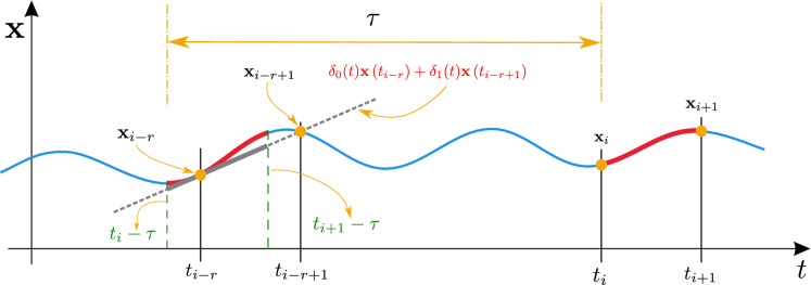
To study the location of the Floquet multipliers, we use the semi-discretization method which is an efficient numerical method based on a special kind of discretization technique with respect to the past effects only [46]. By employing this method, we define a Floquet transition matrix, which is an approximation to the infinite-dimensional monodromy operator U corresponding to the linear delayed system (21). Usually, the semi-discretization method is used to study the linear stability when the system is non-autonomous (contains time-dependent periodic delays or coefficients functions). However, since system (21) is autonomous, we can choose an arbitrary period [43]. Consequently, we assume a period T for the system (21), and hence, the length of the discretization interval is $h=T/K$ where K is the number of subintervals of [0, T]. Let $t_i=ih$. Then, in each discretization interval $[t_i,t_{i+1}]$, the first-order semi-discretization approximate the delayed term $\mathbf{x}(t-\tau )$ by the Lagrange first-order polynomial

$$\begin{array}{c}\hfill \begin{array}{c}\hfill \mathbf{x}(t-\tau )\approx {\delta }_0(t)\mathbf{x}(t_{i-r})+{\delta }_1(t)\mathbf{x}(t_{i-r+1}),\end{array}\end{array}$$ 23

where

$$\begin{array}{cc}& {\delta }_0(t)=\frac{\tau +(i-r+1)h-t}{h},\hfill \\ \hfill & {\delta }_1(t)=\frac{t-(i-r)h-\tau }{h}\hfill \end{array}$$

and $r=\mathrm{int}(\tau /h+1/2)$ with $\mathrm{int}$ denoting the integer-part function, see [43, 44]. The scheme of the approximation in (23) is shown in Fig. 2, and more details are provided in [44, Chapter 3].

Fig. 2.

Approximation of the delayed term $\mathbf{x}(t-\tau )$ is shown by the gray dashed line. Here ${\mathbf{x}}_i=\mathbf{x}(t_i)$

Consequently, system (21) can be approximated by a system of ordinary differential equations

$$\begin{array}{c}\hfill \begin{array}{cc}& \frac{\mathrm{d}\mathbf{x}}{\mathrm{d}t}=\mathbf{A}\mathbf{x}(t)+\mathbf{B}\left({\delta }_0(t)\mathbf{x}(t_{i-r})+{\delta }_1(t)\mathbf{x}(t_{i-r+1})\right),\hfill \\ \hfill & t\in [t_i,t_{i+1}]\hfill \end{array}\end{array}$$ 24

where $i=0,\dots ,K-1$. By using the variation of constants formula, the general solution of (24) can be written as

$$\begin{array}{cc}\hfill \mathbf{X}\left(t\right)=& {\mathrm{e}}^{\mathbf{A}(t-t_i)}\mathbf{X}(t_i)+\underset{t_i}{\overset{t}{\int }}{\mathrm{e}}^{\mathbf{A}(t-s)}\mathbf{B}\hfill \\ \hfill & \left({\delta }_0(t)\mathbf{x}(t_{i-r})+{\delta }_1(t)\mathbf{x}(t_{i-r+1})\right)\mathrm{d}s.\hfill \end{array}$$

Using the notation $\mathbf{x}(t_i)={\mathbf{x}}_i$, when $t=t_{i+1}$. Then, the solution over one discrete step can be formulated as

$$\begin{array}{c}\hfill {\mathbf{x}}_{i+1}=\mathbf{P}{\mathbf{x}}_i+{\mathbf{R}}_{i,0}{\mathbf{x}}_{i-\mathrm{r}}+{\mathbf{R}}_{i,1}{\mathbf{x}}_{i-\mathrm{r}+1},\end{array}$$

where $\mathbf{P}={\mathrm{e}}^{\mathbf{A}h}$ and

$$\begin{array}{c}\hfill \begin{array}{cc}\hfill {\mathbf{R}}_{i,0}& =\left(\underset{0}{\overset{h}{\int }}\frac{\tau -(r-1)h-s}{h}{\mathrm{e}}^{\mathbf{A}(h-s)}\mathrm{d}s\right)\mathbf{B},\hfill \\ \hfill {\mathbf{R}}_{i,1}& =\left(\underset{0}{\overset{h}{\int }}\frac{s+rh-\tau }{h}{\mathrm{e}}^{\mathbf{A}(h-s)}\mathrm{d}s\right)\mathbf{B}.\hfill \end{array}\end{array}$$ 25

If ${\mathbf{A}}^{-1}$ exists, then (25) can be written as

$$\begin{array}{cc}\hfill {\mathbf{R}}_{i,0}& =\left({\mathbf{A}}^{-1},+,\frac{1}{h},\left({\mathbf{A}}^{-2}-\left(\tau -(r-1)h\right){\mathbf{A}}^{-1}\right)\right)\hfill \\ \hfill & \left(\left(I-{\mathrm{e}}^{\mathbf{A}h}\right)\right)\mathbf{B},\hfill \\ \hfill {\mathbf{R}}_{i,1}& =\left(-,{\mathbf{A}}^{-1},+,\frac{1}{h},\left(-{\mathbf{A}}^{-2}-\left(\tau -rh\right){\mathbf{A}}^{-1}\right)\right)\hfill \\ \hfill & \left(\left(I-{\mathrm{e}}^{\mathbf{A}h}\right)\right)\mathbf{B}.\hfill \end{array}$$

Now, we define the augmented state vector as

$$\begin{array}{c}\hfill \begin{array}{c}\hfill {\mathbf{z}}_i={\left({\mathbf{x}}_i,{\mathbf{x}}_{i-1},\dots ,{\mathbf{x}}_{i-\mathrm{r}}\right)}^T.\end{array}\end{array}$$ 26

Combining ${\mathbf{z}}_i$ and (24) leads to the discrete map

$$\begin{array}{c}\hfill {\mathbf{z}}_{i+1}={\mathbf{G}}_i{\mathbf{z}}_i\end{array}$$

where ${\mathbf{G}}_i$ is the coefficient matrix of the form

Utilizing that $T=Kh$ and applying (26) K times with initial state ${\mathbf{z}}_0$ gives the monodromy mapping

$$\begin{array}{c}\hfill \begin{array}{c}\hfill {\mathbf{z}}_{\mathrm{K}}=\mathrm{\Phi }{\mathbf{z}}_0.\end{array}\end{array}$$ 27

where

$$\begin{array}{c}\hfill \mathrm{\Phi }={\mathbf{G}}_{\mathrm{K}-1}{\mathbf{G}}_{\mathrm{K}-2}\cdots {\mathbf{G}}_0\end{array}$$ 28

which represents a finite-dimensional approximation of the monodromy operator U associated with $E_1$ of (2). The rate of convergence for the first-order semi-discretization method is $\mathcal{O}(h^3)$.

When all the eigenvalues of $\mathrm{\Phi }$ are inside the unit circle of the complex plane, then $E_1$ is asymptotically stable. While when one or more of the eigenvalues are on the unit circle and the rest of them are inside the unit circle, $E_1$ may undergo a bifurcation [45]. In the numerical simulations, Sect. 7.4, we implement the above algorithm to construct an approximate stability region for $E_1$. We notice that when $E_1$ is unstable, the model exhibits periodic oscillations as it is expected from SIRS models with delay [47].

The critical vaccination coverage

In this section, we discuss the critical vaccination coverage rate that eliminates the disease. Let ${\mathcal{R}}_E(\psi ):={\mathcal{R}}_E$. When the vaccination is absent, i.e., $\psi =0$, the effective reproduction number becomes

$$\begin{array}{c}\hfill {\mathcal{R}}_0:={\mathcal{R}}_E(0)=\frac{\beta \mathrm{\Lambda }(\alpha +\mu )(\eta +\mu ){\mathrm{e}}^{-\mu \tau }}{\mu (\gamma +\mu )(\alpha (\eta +\mu )+\mu (\eta +\mu ))}.\\ \hfill \end{array}$$ 29

In fact ${\mathcal{R}}_0$ is so-called the basic reproduction number which is the average number of secondary cases arising from one infectious individual in a totally susceptible population [48, 49]. In the case of ${\mathcal{R}}_0$, everyone is susceptible while in ${\mathcal{R}}_E$ not all contacts will become infected due immunity, hence, ${\mathcal{R}}_E$ is less than ${\mathcal{R}}_0$ from epidemiological point of view. Notice that, ${\mathcal{R}}_E(\psi )$ can be written as

$$\begin{array}{c}\hfill {\mathcal{R}}_E(\psi )=\left(\frac{(\alpha +\mu )(\eta +\mu +\xi \psi )}{\alpha (\eta +\mu +\psi )+(\eta +\mu )(\mu +\psi )}\right){\mathcal{R}}_0.\end{array}$$

Thus,

$$\begin{array}{c}\hfill {\mathcal{R}}_E(\infty ):=\underset{\psi \to \infty }{lim}{\mathcal{R}}_E(\psi )=\frac{\xi (\alpha +\mu )}{\alpha +\eta +\mu }{\mathcal{R}}_0.\end{array}$$

Since

$$\begin{array}{cc}& \frac{\mathrm{d}{\mathcal{R}}_E(\psi )}{\mathrm{d}\psi }\hfill \\ \hfill & =-\frac{(\eta +\mu )((1-\xi )(\mu +\alpha )+\eta )}{(\alpha (\eta +\mu +\psi )+(\eta +\mu )(\mu +\psi ))(\eta +\mu +\xi \psi )}{\mathcal{R}}_E(\psi )\hfill \\ \hfill & <0,\hfill \end{array}$$

we have that $\frac{\xi (\alpha +\mu )}{\alpha +\eta +\mu }{\mathcal{R}}_0\le {\mathcal{R}}_E\le {\mathcal{R}}_0$, and hence, ${\mathcal{R}}_0<1$ implies ${\mathcal{R}}_E<1$, but the reverse is not true.

Now, we find the critical level of vaccination to eradicate of the disease when ${\mathcal{R}}_0>1$. Assume ${\mathcal{R}}_0>1$, then

$$\begin{array}{c}\hfill \begin{array}{cc}& {\mathcal{R}}_E(\infty )<1\iff \frac{\xi (\alpha +\mu )}{\alpha +\eta +\mu }{\mathcal{R}}_0<1\iff \hfill \\ \hfill & \xi <\frac{\alpha +\eta +\mu }{\alpha +\mu }\times \frac{1}{{\mathcal{R}}_0}:={\xi }^{\ast }\iff \hfill \\ \hfill & \epsilon >{\epsilon }^{\ast }:=\left(1-\frac{\alpha +\eta +\mu }{\alpha +\mu }\times \frac{1}{{\mathcal{R}}_0}\right).\hfill \end{array}\end{array}$$

Obviously ${ϵ}^{\ast }$ increases as ${\mathcal{R}}_0$ increases. Hence, when $ϵ$ (the vaccine efficacy) is not large enough when ${\mathcal{R}}_0$ is high, the disease may not be eradicated even if everybody gets the vaccine. That is, ${\mathcal{R}}_E(\psi )$ cannot become below 1 when $\psi$ becomes high, see Fig.  3.

Fig. 3.

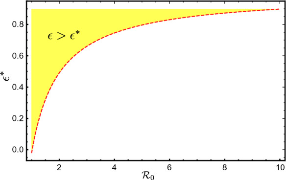
Plot of ${\epsilon }^{\ast }$ as a function of ${\mathcal{R}}_0$

Lemma 1

Assume ${\mathcal{R}}_0>1$. Then, there exists

$$\begin{array}{c}\hfill {\psi }^{\ast }=\frac{({\mathcal{R}}_0-1)\left(\mu +\eta \right)}{{\mathcal{R}}_0\left({\xi }^{\ast }-\xi \right)}=\frac{({\mathcal{R}}_0-1)\left(\mu +\eta \right)}{{\mathcal{R}}_0\left({\xi }^{\ast }+ϵ-1\right)}>0\end{array}$$

such that ${\mathcal{R}}_E({\psi }^{\ast })=1$. Furthermore, ${\mathcal{R}}_E(\psi )>(<)1$ when $\psi <(>){\psi }^{\ast }$.

Biologically, Lemma 1 indicates that ${\psi }^{\ast }$ is the vaccination coverage rate to eradicate of the disease.

From $V^0$ and Theorem 2.1, we have

$$\begin{array}{cc}\hfill V^0=& \frac{\mathrm{\Lambda }}{\mu }\times \frac{\psi (\alpha +\mu )}{\alpha (\eta +\mu +\psi )+(\eta +\mu )(\mu +\psi )}\hfill \\ \hfill =& N(t)\times \frac{\psi (\alpha +\mu )}{\alpha (\eta +\mu +\psi )+(\eta +\mu )(\mu +\psi )}.\hfill \end{array}$$

Hence,

$$\begin{array}{c}\hfill \frac{V^0}{N(t)}=\frac{\psi (\alpha +\mu )}{\alpha (\eta +\mu +\psi )+(\eta +\mu )(\mu +\psi )}.\end{array}$$ 30

Hence, in a disease-free population, the proportion of vaccinated individuals is

$$\begin{array}{c}\hfill \frac{\psi (\alpha +\mu )}{\alpha (\eta +\mu +\psi )+(\eta +\mu )(\mu +\psi )}.\end{array}$$ 31

Therefore, when ${\mathcal{R}}_0>1$, the critical proportion of the population that should be vaccinated when the vaccination is imperfect and $\psi ={\psi }^{\ast }$ is given by

$$\begin{array}{c}\hfill {\rho }_{\epsilon }=\frac{({\mathcal{R}}_0-1)\left(\mu +\eta \right)(\alpha +\mu )}{({\mathcal{R}}_0-1)\left(\mu +\eta \right)(\alpha +\eta +\mu )+{\mathcal{R}}_0\left({\xi }^{\ast }+\epsilon -1\right)(\alpha +\mu )(\eta +\mu )}.\\ \hfill \end{array}$$ 32

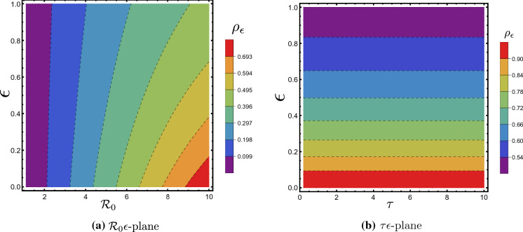
Figure 4a and b shows the contour plot of ${\rho }_{\epsilon }$ in ${\mathcal{R}}_0ϵ$- and $\tau ϵ$-plane, respectively. We notice that when $ϵ$ is fixed, ${\rho }_{\epsilon }$ increases as ${\mathcal{R}}_0$ increases. While $\tau$ does not have a noticeable effect on the value of ${\rho }_{\epsilon }$. Also, the figures are consistent with that fact that $\frac{\partial {\rho }_{\epsilon }}{\partial \epsilon }\le 0$.

Fig. 4.

The contour plot of ${\rho }_{\epsilon }$. Parameters values are similar to those in Fig. 5

Numerical simulations

In this section, firstly, we fit the model with data of influenza patients as a case study. Secondly, we study the local and global sensitivity of ${\mathcal{R}}_E$ with respect to the parameters of system (2). Thirdly, we discuss the stability of endemic equilibrium. Finally, we investigate the sensitivity system of the system (2) with respect to main parameters.

Through this section, we take

$$\begin{array}{c}\hfill f(I)=1+0.001I^5.\end{array}$$

Case study

We use the system (2) to simulate the data of influenza patients (weekly percentage) in North Carolina from January to April, 2011 [50]. A range for (2) parameters is given in Table 2. Figure 5 shows that the numerical solution of (2) provides a good agreement with the real data.

Table 2.

Parameter value ranges of the system (2)

Parameter	Range	Reference
$\beta$	[0.390, 0.432] per day	[25]
$\psi$	[0.371, 0.436]	[51]
$\alpha$	Six months	[52]
$\xi$	[0.4, 0.81]	[53]
$1/\eta$	Two weeks	[54]
$\tau$	[1, 4]	[55]
Infectious period ($1/\gamma$)	[3, 7] days	[55]

Fig. 5.

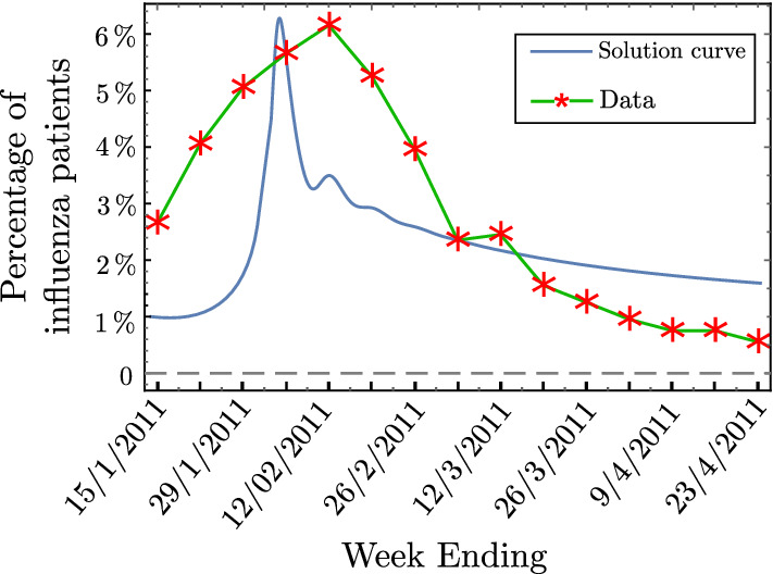
Weekly percentage of influenza patients in North Carolina from January to April, 2011 [50] compared to the simulation results of the system (2). Parameters: $\beta =0.196$ per week, $\gamma =2$, $\alpha =16$ weeks, $\eta =0.5$ per week, $\mathrm{\Lambda }=100$, $\mu =0.1$, $\xi =0.3$, $\psi =0.4$, $\tau =0.143$ week. Initial functions: $S(\theta )=100$, $I(\theta )=1$, $V(\theta )=E(\theta )=R(\theta )=0$ for $\theta \in [-0.143,0]$

Local sensitivity of ${\mathcal{R}}_E$

The local sensitivity analysis of ${\mathcal{R}}_E$ provides insight into the proportional change in ${\mathcal{R}}_E$ responding to a small variation of a single parameter p at one time. The normalized forward sensitivity index of ${\mathcal{R}}_E$ (elasticity of ${\mathcal{R}}_E$) measures such relative change in ${\mathcal{R}}_E$, denoted by ${\mathrm{{\rm Y}}}_p^{{\mathcal{R}}_E}$, and defined as [56, 57]:

$$\begin{array}{c}\hfill \begin{array}{c}\hfill {\mathrm{{\rm Y}}}_p^{{\mathcal{R}}_E}:=\frac{\partial {\mathcal{R}}_E}{\partial p}\times \frac{p}{{\mathcal{R}}_E}.\end{array}\end{array}$$ 33

From the explicit formula of ${\mathcal{R}}_E$ in (7), we derive an analytical expression for ${\mathrm{{\rm Y}}}_p^{{\mathcal{R}}_E}$ to each parameter described in Table 1. From (7) and (33), we have

$$\begin{array}{cc}\hfill {\mathrm{{\rm Y}}}_{\mathrm{\Lambda }}^{{\mathcal{R}}_E}& ={\mathrm{{\rm Y}}}_{\beta }^{{\mathcal{R}}_E}=1,\hfill \\ \hfill {\mathrm{{\rm Y}}}_{\psi }^{{\mathcal{R}}_E}& =-\frac{\psi \eta (\eta +\mu )(1-\xi )(\alpha +\mu )}{(\alpha (\eta +\mu +\psi )+(\eta +\mu )(\mu +\psi ))(\eta +\mu +\xi \psi )}\hfill \\ \hfill & <0,\hfill \\ \hfill {\mathrm{{\rm Y}}}_{\mu }^{{\mathcal{R}}_E}& =-\mu \tau -1-\frac{\mu (\alpha +\eta +2\mu +\psi )}{\alpha (\eta +\mu +\psi )+(\eta +\mu )(\mu +\psi )}\hfill \\ \hfill & +\frac{\mu }{\alpha +\mu }-\frac{\mu }{\gamma +\mu }+\frac{\mu }{\eta +\mu +\xi \psi },\hfill \\ \hfill {\mathrm{{\rm Y}}}_{\eta }^{{\mathcal{R}}_E}& =-\frac{\eta \psi (\alpha (\xi -1)+\xi (\mu +\psi ))}{(\alpha (\eta +\mu +\psi )+(\eta +\mu )(\mu +\psi ))(\eta +\mu +\xi \psi )},\hfill \\ \hfill {\mathrm{{\rm Y}}}_{\gamma }^{{\mathcal{R}}_E}& =-\frac{\gamma }{\gamma +\mu }<0,\hfill \\ \hfill {\mathrm{{\rm Y}}}_{\alpha }^{{\mathcal{R}}_E}& =\frac{(\alpha \eta \psi )}{(\alpha +\mu )(\alpha (\eta +\mu +\psi )+(\eta +\mu )(\mu +\psi ))}\hfill \\ \hfill & <0,\hfill \\ \hfill {\mathrm{{\rm Y}}}_{\tau }^{{\mathcal{R}}_E}& =-\mu \tau <0.\hfill \end{array}$$ 34

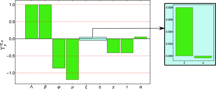
First, we notice for the parameters $\mathrm{\Lambda }$ and $\beta$, the sensitivity indices ${\mathrm{{\rm Y}}}_{\mathrm{\Lambda }}^{{\mathcal{R}}_E}$ and ${\mathrm{{\rm Y}}}_{\beta }^{{\mathcal{R}}_E}$ are independent of any other parameters; hence, they are locally and globally valid. Also, both parameters are equally important for ${\mathcal{R}}_E$ because ${\mathrm{{\rm Y}}}_{\mathrm{\Lambda }}^{{\mathcal{R}}_E}={\mathrm{{\rm Y}}}_{\beta }^{{\mathcal{R}}_E}=1$. Consequently, when $\mathrm{\Lambda }$ or $\beta$ increases by $100\%$, then ${\mathcal{R}}_E$ increases by $100\%$. For the other parameters $p\in \{\psi ,\mu ,\xi ,\eta ,\tau ,\gamma ,\delta \}$, they have different impacts on ${\mathcal{R}}_E$ due to the different absolute value of the forward sensitivity indices ${\mathrm{{\rm Y}}}_p^{{\mathcal{R}}_E}$ in (34). We use the values in Table 2 to calculate numeric values for ${\mathrm{{\rm Y}}}_p^{{\mathcal{R}}_E}$, see Fig. 6. For example, when $\psi$ increases by $100\%$, ${\mathcal{R}}_E$ decreases by $86\%$ while when $\alpha$ increases by $100\%$, ${\mathcal{R}}_E$ increases by $5\%$; hence, due to absolute value of the sensitivity index we have $\varphi$ is more important for ${\mathcal{R}}_E$. From Fig. 6, we notice that the order of parameters from the highest importance to the lowest is $\mu$, $\mathrm{\Lambda }$(and $\beta$), $\psi$, $\gamma$, $\tau$, $\alpha$, $\xi$ and $\eta$.

Fig. 6.

Local sensitivity indices of ${\mathcal{R}}_E$

Global sensitivity of ${\mathcal{R}}_E$

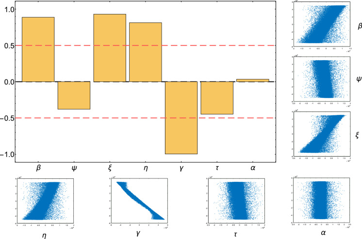
When there are large perturbations in all parameters, global sensitivity analysis is typically used which includes sampling a given range of parameter values [58]. We use the Latin Hypercube Sampling (LHS) design and Partial Rank Correlation Coefficient (PRCC) analysis technique to provide good insight on global sensitivity of ${\mathcal{R}}_E$ on the uncertainties in its parameters [59]. The PRCC values vary in the interval $[-1,1]$ such that there is a perfect negative$\backslash$positive correlation when the value is $-1\backslash 1$, also, the PRCC value is statistically significant when |PRCC value$|>0.5$. Figure 7 shows PRCC values of ${\mathcal{R}}_E$ where the parameters sampling are produced from LHS with uniform distribution over the parameter values in Table 2 with 1,000,000 samples. We notice from Fig. 7 that the most influential parameters on ${\mathcal{R}}_E$, ordered from highest to lowest, are $\gamma$, $\xi$, $\beta$, $\eta$, $\tau$, $\psi$ and $\alpha$.

Fig. 7.

PRCC results, the orange boxes represent the partial rank correlation coefficients of ${\mathcal{R}}_E$. The small figures in the right side and bottom show the PRCC scatter plots

Stability of $E_1$

In this section, we fix

$$\begin{array}{c}\hfill \mathrm{\Lambda }=300,\eta =1,\mu =0.13,\xi =\alpha =0.01.\end{array}$$

We use the package SemiDiscretizationMethod.jl on Julia to implement the algorithm in Sect. 5.1 and construct an approximate stability region for $E_1$ in two parameters space. Figure 8 shows the stability charts in $\beta \gamma$-plane, $\beta \psi$-plane and $\gamma \psi$-plane. In Fig. 8b, when $\psi$ is fixed in the interval [0.4, 0.6] and $\beta$ increases, a stability switches occur where endemic equilibrium losses its stability and then becomes stable for larger $\beta$, see Fig. 9a. While when $\beta$ is fixed and $\psi$ increases, a Hopf bifurcation occurs and the endemic equilibrium losses its stability and becomes unstable, see Fig. 9b. The latter case also occurs when $\beta$ or $\psi$ is fixed and $\gamma$ increases, see Fig. 8a and c.

Fig. 8.

Stability chart for the endemic equilibrium $E_1$ obtained by semi-discretization method for $h=0.1$, where stable region is the green area and unstable region is the gray area

Fig. 9.

One-parameter bifurcation diagrams with $\beta$, $\psi$ and $\tau$. We fix $\gamma =0.09$

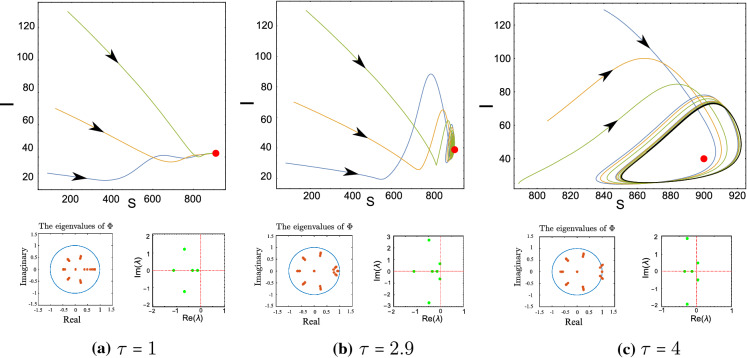
Figure 9c shows a one-parameter bifurcation diagram, by varying the value of $\tau$. For small $\tau$, the endemic equilibrium $E_1$ is stable (Fig. 10a). By increasing the value of $\tau$, $E_1$ loses the stability and a Hopf Bifurcation occurs around $\tau \approx 2.94$. For $\tau >2.94$, a unique stable periodic solution of system (2) exists (Fig. 10c). In Fig. 10, we plot the phase portrait of the system (2) with different initial condition and various value of $\tau$, we notice that system (2) exhibits global asymptotic stability behavior when ${\mathcal{R}}_E>1$.

Fig. 10.

Row 1: phase portrait of the system (2) with different initial condition and various value of $\tau$. Row 2: the eigenvalues of the matrix $\mathrm{\Phi }$ in (28) and the roots of the characteristic equation corresponding to $E_1$. $\beta =0.9,\gamma =0.09$ and $\psi =0.2$ The endemic equilibrium $E_1$ is a (912.618, 161.509, 1.30009, 42.5669, 1181 b (905.814, 160.301, 4.02373, 39.9422, 1170.68) c (901.278, 159.496, 5.77535, 38.4905, 1164)

Sensitivity of model solutions

The sensitivity system of (2) with respect to a parameter $p\in \{\psi ,\mu ,\xi ,\eta ,\tau ,\gamma ,\alpha \}$ is given by the partial derivative of $\mathbf{X}={(S,V,E,I,R)}^T$ with respect to p, denoted by ${\mathbf{X}}_p=\frac{\partial \mathbf{X}}{\partial p}$. Define $\mathbf{f}(S,V,E,I,R):=\frac{\mathrm{d}\mathbf{X}}{\mathrm{d}t}$, then by the Chain Rule and Clairaut’s Theorem, we have

$$\begin{array}{c}\hfill \frac{\mathrm{d}{\mathbf{X}}_p}{\mathrm{d}t}=\frac{\mathrm{d}\mathbf{f}}{\mathrm{d}\mathbf{X}}{\mathbf{X}}_p+\frac{\partial \mathbf{f}}{\partial p},{\mathbf{X}}_p(0)=\frac{\partial {\mathbf{X}}_0(p)}{\partial p}.\end{array}$$

The semi-relative sensitivity for $\mathbf{X}$ is represented by $p{\mathbf{X}}_p$, while the logarithmic sensitivity is represented by $p\frac{{\mathbf{X}}_p}{\mathbf{X}}$. The detailed method is given in [60].

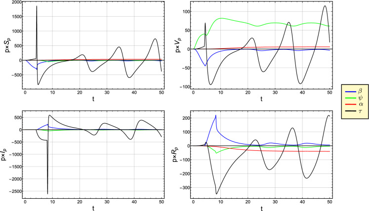
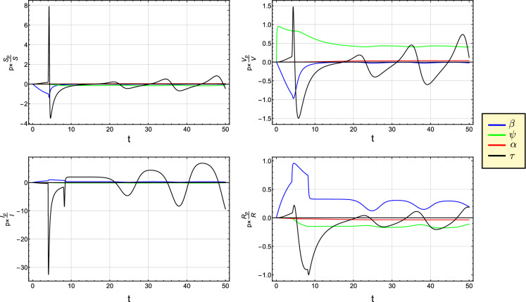
Figures 11 and 12 show the semi-relative and logarithmic sensitivity curves for S, V, I and R with respect to the parameter $\beta$, $\psi$, $\alpha$ and $\tau$. From Figs. 11 and 12, we can interpret that the perturbation of $\tau$ has a big influence over S, V, I and R. For $t\in (0,10)$, a remarkable positive affect of the parameter $\beta$ occurs on I and R, while an opposite affect appears on the variables S and V. Moreover, at $t\approx 4(7)$, we notice that both parameters $\tau$ and $\beta$ have the largest effects on S and V (I and R). The perturbation of $\psi$ and $\alpha$ has a noticeable positive affect on V and R.

Fig. 11.

The semi-relative sensitivity curves of S, V, I and R with respect to the parameter $\beta$, $\psi$, $\alpha$ and $\tau$

Fig. 12.

The logarithmic sensitivity curves of S, V, I and R with respect to the parameter $\beta$, $\psi$, $\alpha$ and $\tau$

Finally, since the function f(I) is independent of the value of ${\mathcal{R}}_E$, we consider $f(I)=1+d{I}^q$ and study the influence of the parameters d and q on the solution of the system (2). In Fig. 13, the sensitivity solution curves show that d and q have a positive influences on S and V and a negative affects on I. The influence of q is relatively higher than that of d. More precisely, q has an oscillatory influence on $\{S,V,I,R\}$. There are small affects (around zero) of d on the four variables.

Fig. 13.

The semi-relative (row 1) and logarithmic (row 2) sensitivity curves for S, V, I and R with respect to the parameter d (red) and q (green) in $f(I)=1+d{I}^q$

Conclusions

Nowadays, epidemiological modeling plays a key role in providing strategies for the prevention and control of many communicable diseases. Vaccination, meanwhile, is considered to be one of the most favored and effective methods of mitigation and elimination of epidemics. In the paper, we have studied infectious disease transmission dynamics in the presence of an imperfect vaccine by a stage-structured mathematical model. To interpret the “psychological effect” when an infectious disease being spread in a population, we have considered a general nonmonotone nonlinear incidence rate function. We have shown that the solutions of the proposed model exist (uniquely determined) and they are nonnegative and bounded, that is, the model is biologically well-posed.

Due to the existence of time delay, we have used the method in [35] to obtain an explicit expression for the effective reproduction number (${\mathcal{R}}_E$) which gives the actual number of secondary infections per infectious person at any time [16, 36]. Then we have obtained the threshold dynamics of the system with respect to ${\mathcal{R}}_E$: (i) we have shown that the disease-free equilibrium is globally stable when ${\mathcal{R}}_E<1$; and (ii) we have discussed the system persistence and the coexistence of endemic equilibrium when ${\mathcal{R}}_E>1$. Then, we have used the semi-discretization method to analyze the linear stability of the endemic equilibrium. Also, we have discussed the critical vaccination coverage rate that is required to eliminate the disease and the critical proportion of the population (${\rho }_{ϵ}$) that should be vaccinated when the vaccination is imperfect. We have not noticed any influence of the latent time $\tau$ on ${\rho }_{ϵ}$ when the vaccine efficacy $ϵ$ is fixed. However, we have observed that the value of ${\rho }_{ϵ}$ increases as ${\mathcal{R}}_0$ increases when $ϵ$ is fixed. The quantity ${\mathcal{R}}_0$ is the value of ${\mathcal{R}}_E$ when the vaccination rate $\psi$ is zero. Furthermore, through the theoretical analysis, we have found that when $ϵ$ is not large enough and ${\mathcal{R}}_0$ is high, the disease may not be eradicated even if everybody gets the vaccine. In other words, ${\mathcal{R}}_E$ cannot become below the unity even when $\psi$ becomes high.

Through the numerical simulations:

• We have fitted the model with data of influenza patients as a case study. We have noticed that at the peak level of infection, nearly $6\%$ of the population is infected;

• We have carried out global and local sensitivities analysis for ${\mathcal{R}}_E$. We have found that the latent time $\tau$ has a noticeable effect on ${\mathcal{R}}_E$. Regarding the vaccination parameters, $\psi$ and the reduction coefficient ($\xi$), they both have an opposite effect on the value of ${\mathcal{R}}_E$, $\psi$ has a negative influence while $\xi$ has a positive one;

• We have constructed an approximate stability region for the endemic equilibrium $E_1$ and noticed that when $E_1$ loses its stability, a unique stable periodic solution exists via Hopf Bifurcation. For example, for small $\tau$, the endemic equilibrium is stable and as the value of $\tau$ increases, $E_1$ loses the stability and a Hopf Bifurcation occurs and a unique stable periodic solution exists. Moreover, we have observed that the model exhibits global asymptotic stability behavior when ${\mathcal{R}}_E>1$.

• The semi-relative and logarithmic sensitivities curves have shown that the perturbation of $\tau$ has a big influence over the variables $\{S,V,I,R\}$.

• Although ${\mathcal{R}}_E$ is independent of the function f, the sensitivity curves of the model solutions have shown f has a noticeable effect on the behavior of the solution.

For further work, it will be interesting to consider the “asymptomatic carriers”. These carriers are individuals who have been infected and are able to transmit their illness without showing any symptoms [3]. For certain infectious diseases, asymptomatic carriers are a potential source for transmission such as Typhoid Fever, HIV and, most recently, the COVID-19.

Compliance with ethical standards

Conflict of interest

The author declares that he has no conflict of interest.

References

- 1.Cooke KL. Stability analysis for a vector disease model. Rocky Mt. J. Math. 1979;9(1):31–42. [Google Scholar]
- 2.Duan X, Yuan S, Qiu Z, Ma J. Global stability of an SVEIR epidemic model with ages of vaccination and latency. Comput. Math. Appl. 2014;68(3):288–308. [Google Scholar]
- 3.Al-Darabsah I, Yuan Y. A periodic disease transmission model with asymptomatic carriage and latency periods. J. Math. Biol. 2018;77(2):343–376. doi: 10.1007/s00285-017-1199-1. [DOI] [PubMed] [Google Scholar]
- 4.Cooke KL, Van Den Driessche P. Analysis of an SEIRS epidemic model with two delays. J. Math. Biol. 1996;35(2):240–260. doi: 10.1007/s002850050051. [DOI] [PubMed] [Google Scholar]
- 5.Van Den Driessche P, Wang L, Zou X. Modeling diseases with latency and relapse. Math. Biosci. Eng. 2007;4(2):205. doi: 10.3934/mbe.2007.4.205. [DOI] [PubMed] [Google Scholar]
- 6.Al-Darabsah I, Yuan Y. A time-delayed epidemic model for ebola disease transmission. Appl. Math. Comput. 2016;290:307–325. [Google Scholar]
- 7.Goel K, et al. Stability behavior of a nonlinear mathematical epidemic transmission model with time delay. Nonlinear Dyn. 2019;98(2):1501–1518. [Google Scholar]
- 8.Xu R. Global stability of a delayed epidemic model with latent period and vaccination strategy. Appl. Math. Model. 2012;36(11):5293–5300. [Google Scholar]
- 9.Agaba G, Kyrychko Y, Blyuss K. Dynamics of vaccination in a time-delayed epidemic model with awareness. Math. Biosci. 2017;294:92–99. doi: 10.1016/j.mbs.2017.09.007. [DOI] [PubMed] [Google Scholar]
- 10.Meng X, Chen L, Wu B. A delay SIR epidemic model with pulse vaccination and incubation times. Nonlinear Anal. Real World Appl. 2010;11(1):88–98. [Google Scholar]
- 11.Gao S, Chen L, Teng Z. Pulse vaccination of an SEIR epidemic model with time delay. Nonlinear Anal. Real World Appl. 2008;9(2):599–607. [Google Scholar]
- 12.Li, K., Zhang, H., Zhu, G., Small, M., Fu, X.: Suboptimal control and targeted constant control for semi-random epidemic networks. IEEE Trans. Syst. Man Cybern. Syst. (2019). 10.1109/TSMC.2019.2916859
- 13.Pastor-Satorras R, Vespignani A. Epidemic spreading in scale-free networks. Phys. Rev. Lett. 2001;86(14):3200. doi: 10.1103/PhysRevLett.86.3200. [DOI] [PubMed] [Google Scholar]
- 14.Farrington C. On vaccine efficacy and reproduction numbers. Math. Biosci. 2003;185(1):89–109. doi: 10.1016/s0025-5564(03)00061-0. [DOI] [PubMed] [Google Scholar]
- 15.Sisodiya OS, Misra O, Dhar J. Dynamics of cholera epidemics with impulsive vaccination and disinfection. Math. Biosci. 2018;298:46–57. doi: 10.1016/j.mbs.2018.02.001. [DOI] [PubMed] [Google Scholar]
- 16.Rao F, Mandal PS, Kang Y. Complicated endemics of an SIRS model with a generalized incidence under preventive vaccination and treatment controls. Appl. Math. Model. 2019;67:38–61. [Google Scholar]
- 17.Liu X, Takeuchi Y, Iwami S. SVIR epidemic models with vaccination strategies. J. Theor. Biol. 2008;253(1):1–11. doi: 10.1016/j.jtbi.2007.10.014. [DOI] [PubMed] [Google Scholar]
- 18.Gumel AB, McCluskey CC, Watmough J. An SVEIR model for assessing potential impact of an imperfect anti-sars vaccine. Math. Biosci. Eng. 2006;3(3):485–512. doi: 10.3934/mbe.2006.3.485. [DOI] [PubMed] [Google Scholar]
- 19.Arino J, Cooke K, Van Den Driessche P, Velasco-Hernández J. An epidemiology model that includes a leaky vaccine with a general waning function. Discrete Contin. Dyn. Syst. Ser. B. 2004;4(2):479. [Google Scholar]
- 20.Lv W, Ke Q, Li K. Dynamical analysis and control strategies of an SIVS epidemic model with imperfect vaccination on scale-free networks. Nonlinear Dyn. 2020;99(2):1507–1523. doi: 10.1007/s11071-019-05371-1. [DOI] [PMC free article] [PubMed] [Google Scholar]
- 21.Liu W-M, Levin SA, Iwasa Y. Influence of nonlinear incidence rates upon the behavior of SIRS epidemiological models. J. Math. Biol. 1986;23(2):187–204. doi: 10.1007/BF00276956. [DOI] [PubMed] [Google Scholar]
- 22.Xiao D, Ruan S. Global analysis of an epidemic model with nonmonotone incidence rate. Math. Biosci. 2007;208(2):419–429. doi: 10.1016/j.mbs.2006.09.025. [DOI] [PMC free article] [PubMed] [Google Scholar]
- 23.Ruan S, Wang W. Dynamical behavior of an epidemic model with a nonlinear incidence rate. J. Differ. Equ. 2003;188(1):135–163. [Google Scholar]
- 24.Lu M, Huang J, Ruan S, Yu P. Bifurcation analysis of an SIRS epidemic model with a generalized nonmonotone and saturated incidence rate. J. Differ. Equ. 2019;267(3):1859–1898. doi: 10.1016/j.jde.2019.03.005. [DOI] [PMC free article] [PubMed] [Google Scholar]
- 25.Tan X, Yuan L, Zhou J, Zheng Y, Yang F. Modeling the initial transmission dynamics of influenza a h1n1 in guangdong province, china. Int. J. Infect. Dis. 2013;17(7):e479–e484. doi: 10.1016/j.ijid.2012.11.018. [DOI] [PubMed] [Google Scholar]
- 26.Duesberg P. Infectious AIDS: Have We Been Misled? Berkeley: North Atlantic Books; 1995. [Google Scholar]
- 27.Svensson Å. A note on generation times in epidemic models. Math. Biosci. 2007;208(1):300–311. doi: 10.1016/j.mbs.2006.10.010. [DOI] [PubMed] [Google Scholar]
- 28.Nelson KE, Williams CM. Infectious Disease Epidemiology: Theory and Practice. Burlington: Jones & Bartlett Publishers; 2014. [Google Scholar]
- 29.Arino J, McCluskey CC, van den Driessche P. Global results for an epidemic model with vaccination that exhibits backward bifurcation. SIAM J. Appl. Math. 2003;64(1):260–276. [Google Scholar]
- 30.Martcheva M. An Introduction to Mathematical Epidemiology. Berlin: Springer; 2015. [Google Scholar]
- 31.Wang W. Backward bifurcation of an epidemic model with treatment. Math. Biosci. 2006;201(1–2):58–71. doi: 10.1016/j.mbs.2005.12.022. [DOI] [PubMed] [Google Scholar]
- 32.Hale JK, Lunel SMV. Introduction to Functional Differential Equations. Berlin: Springer; 2013. [Google Scholar]
- 33.Smith HL. Monotone Dynamical Systems: An Introduction to the Theory of Competitive and Cooperative Systems. Providence: American Mathematical Soc; 2008. [Google Scholar]
- 34.Teschl G. Ordinary Differential Equations and Dynamical Systems. Providence: American Mathematical Soc; 2012. [Google Scholar]
- 35.Zhao X-Q. Basic reproduction ratios for periodic compartmental models with time delay. J. Dyn. Differ. Equ. 2017;29(1):67–82. [Google Scholar]
- 36.Farrington C, Whitaker H. Estimation of effective reproduction numbers for infectious diseases using serological survey data. Biostatistics. 2003;4(4):621–632. doi: 10.1093/biostatistics/4.4.621. [DOI] [PubMed] [Google Scholar]
- 37.LaSalle JP. The Stability of Dynamical Systems. Philadelphia: SIAM; 1976. [Google Scholar]
- 38.Tian Y, Al-Darabsah I, Yuan Y. Global dynamics in sea lice model with stage structure. Nonlinear Anal. Real World Appl. 2018;44:283–304. [Google Scholar]
- 39.Hirsch WM, Hanisch H, Gabriel J-P. Differential equation models of some parasitic infections: methods for the study of asymptotic behavior. Commun. Pure Appl. Math. 1985;38(6):733–753. [Google Scholar]
- 40.Giaquinta M, Modica G. Mathematical Analysis: An Introduction to Functions of Several Variables. Basel: Birkhäuser; 2009. [Google Scholar]
- 41.Smith H, Zhao XQ. Robust persistence for semidynamical systems. Nonlinear Anal. Theory Methods Appl. 2001;47(9):6169–6179. [Google Scholar]
- 42.Zhao X-Q. Permanence implies the existence of interior periodic solutions for FDEs. Int. J. Qual. Theory Differ. Equ. Appl. 2008;2:125–137. [Google Scholar]
- 43.Balachandran B, Kalmár-Nagy T, Gilsinn DE. Delay Differential Equations. Berlin: Springer; 2009. [Google Scholar]
- 44.Insperger T, Stépán G. Semi-discretization for Time-delay Systems: Stability and Engineering Applications. Berlin: Springer; 2011. [Google Scholar]
- 45.Nayfeh AH, Balachandran B. Applied Nonlinear Dynamics: Analytical, Computational, and Experimental Methods. New York: Wiley; 2008. [Google Scholar]
- 46.Insperger T, Stépán G. Semi-discretization method for delayed systems. Int. J. Numer. Methods Eng. 2002;55(5):503–518. [Google Scholar]
- 47.Hethcote HW, Stech HW, Van Den Driessche P. Nonlinear oscillations in epidemic models. SIAM J. Appl. Math. 1981;40(1):1–9. [Google Scholar]
- 48.Guerra FM, Bolotin S, Lim G, Heffernan J, Deeks SL, Li Y, Crowcroft NS. The basic reproduction number () of measles: a systematic review. Lancet Infect. Dis. 2017;17(12):e420–e428. doi: 10.1016/S1473-3099(17)30307-9. [DOI] [PubMed] [Google Scholar]
- 49.Van den Driessche P, Watmough J. Reproduction numbers and sub-threshold endemic equilibria for compartmental models of disease transmission. Math. Biosci. 2002;180(1–2):29–48. doi: 10.1016/s0025-5564(02)00108-6. [DOI] [PubMed] [Google Scholar]
- 50.Yarmand H, Ivy JS, Denton B, Lloyd AL. Optimal two-phase vaccine allocation to geographically different regions under uncertainty. Eur. J. Oper. Res. 2014;233(1):208–219. [Google Scholar]
- 51.CDC: Estimates of influenza vaccination coverage among adults in the United States. https://www.cdc.gov/flu/fluvaxview/coverage-1718estimates.htm. Accessed 20 Oct 2019
- 52.IAC: Ask the experts—influenza. https://www.immunize.org/askexperts/experts_inf.asp. Accessed 29 Oct 2019
- 53.CDC: Past seasons vaccine effectiveness estimates. https://www.cdc.gov/flu/vaccines-work/past-seasons-estimates.html. Accessed 15 Oct 2019
- 54.WHO: Key facts about seasonal flu vaccine. https://www.cdc.gov/flu/prevent/keyfacts.htm. Accessed 10 Oct 2019
- 55.WHO: How flu spreads. https://www.cdc.gov/flu/about/disease/spread.htm. Accessed 10 Oct 2019
- 56.Chitnis N, Hyman JM, Cushing JM. Determining important parameters in the spread of malaria through the sensitivity analysis of a mathematical model. Bull. Math. Biol. 2008;70(5):1272. doi: 10.1007/s11538-008-9299-0. [DOI] [PubMed] [Google Scholar]
- 57.van den Driessche P. Reproduction numbers of infectious disease models. Infect. Dis. Model. 2017;2(3):288–303. doi: 10.1016/j.idm.2017.06.002. [DOI] [PMC free article] [PubMed] [Google Scholar]
- 58.Ingalls BP. Mathematical Modeling in Systems Biology: An Introduction. New York: MIT press; 2013. [Google Scholar]
- 59.Marino S, Hogue IB, Ray CJ, Kirschner DE. A methodology for performing global uncertainty and sensitivity analysis in systems biology. J. Theor. Biol. 2008;254(1):178–196. doi: 10.1016/j.jtbi.2008.04.011. [DOI] [PMC free article] [PubMed] [Google Scholar]
- 60.Bortz D, Nelson P. Sensitivity analysis of a nonlinear lumped parameter model of HIV infection dynamics. Bull. Math. Biol. 2004;66(5):1009–1026. doi: 10.1016/j.bulm.2003.10.011. [DOI] [PubMed] [Google Scholar]