Developing risk models for multicenter data using standard logistic regression produced suboptimal predictions: A simulation study

Abstract

Although multicenter data are common, many prediction model studies ignore this during model development. The objective of this study is to evaluate the predictive performance of regression methods for developing clinical risk prediction models using multicenter data, and provide guidelines for practice. We compared the predictive performance of standard logistic regression, generalized estimating equations, random intercept logistic regression, and fixed effects logistic regression. First, we presented a case study on the diagnosis of ovarian cancer. Subsequently, a simulation study investigated the performance of the different models as a function of the amount of clustering, development sample size, distribution of center‐specific intercepts, the presence of a center‐predictor interaction, and the presence of a dependency between center effects and predictors. The results showed that when sample sizes were sufficiently large, conditional models yielded calibrated predictions, whereas marginal models yielded miscalibrated predictions. Small sample sizes led to overfitting and unreliable predictions. This miscalibration was worse with more heavily clustered data. Calibration of random intercept logistic regression was better than that of standard logistic regression even when center‐specific intercepts were not normally distributed, a center‐predictor interaction was present, center effects and predictors were dependent, or when the model was applied in a new center. Therefore, to make reliable predictions in a specific center, we recommend random intercept logistic regression.

1. INTRODUCTION

Clinical risk prediction models have the purpose of enhancing personalized medicine: they yield personalized risk estimates based on several predictors. When performing clinical studies, multicenter data is often used. For example, 64% of the models published after the year 2000 in the Tufts PACE Clinical Prediction Model Registry are developed on multicenter data (Wynants, Kent, Timmerman, Lunquist, & Van Calster, 2019). This practice has two advantages: enhancing the efficiency of the data collection process as well as the generalizability of results. However, data are no longer independent, because patients within the same center tend to be more similar than patients from different centers (“clustering”) (Snijders & Bosker, 2012).

Although multicenter data are common, many prediction model studies ignore this during model development. In a random selection of 50 multicenter studies from the Tufts Registry, only 11 studies addressed the multicenter nature in some aspect of the analysis (Wynants et al., 2019).

Methodology for clustered data in randomized clinical trials is well developed. This is not the case for prediction research. There are several ways to take into account clustering: random effects models, fixed effects models including dummies for all minus 1 cluster (i.e., center), and generalized estimating equations. Previous studies claim that fixed effects models should be used to analyze trial data when there are few centers and when the number of people in each center is sufficiently large (Kahan, 2014; Kahan & Harhay, 2015). The number of coefficients to be estimated increases with the number of centers, and estimates become less precise as the number of patients per center decreases. In contrast, for the random intercept model, only one extra variable needs to be estimated: the random intercept variance. However, this requires the assumption of normality for the center effects. It is also thought that random intercept models should only be used when there is an adequate number of centers to make sure there is sufficient information to estimate the random intercept variance (Kahan, 2014; Kahan & Harhay, 2015; Moineddin, Matheson, & Glazier, 2007).

Usually, prediction models are intended to be broadly applied in a wide variety of clinical centers. When validating the model performance, it should be investigated whether the model performs well within individual centers. It has therefore been recommended to use within‐center performance measures, which also allow to investigate heterogeneity in performance between centers (Meisner, Parikh, & Kerr, 2017; Van Klaveren, Steyerberg, Perel, & Vergouwe, 2014; Wynants, Vergouwe, Van Huffel, Timmerman, & Van Calster, 2018).

This paper compares different approaches to account for multicenter data when developing risk prediction models. We demonstrate the modeling approaches in a case study to diagnose ovarian cancer and perform a simulation study to investigate different possible scenarios. Based on our findings, we formulate recommendations for practice.

2. MOTIVATING CASE STUDY: DIAGNOSIS OF OVARIAN CANCER

When a suspicious ovarian tumor is detected, it is important to predict whether it is malignant prior to surgery. High‐risk tumors should then be referred for specialized oncological care, whereas low‐risk tumors may be treated locally. We developed and validated risk models for ovarian malignancy on data from the International Ovarian Tumor Analysis group (IOTA). Data from IOTA phases 1, 1B, and 2 (1999–2007, n = 3,506, 21 centers) (Timmerman et al., 2005, 2010; Van Holsbeke et al., 2009) were used for model development. Data from phase 3 (2009–2012, n = 2,403, 18 center) (Testa et al., 2014) were used to externally validate model performance. The validation data included data from 15 centers that also contributed to the development dataset, as well as data from three new centers. Overall, the data included 5,909 patients from 24 different centers. The number of patients per center was on average 246 (range 11 to 930). The prevalence of malignant tumors was 33% but center‐specific prevalences ranged from 0 to 66%, reflecting differences in the specialization of centers in ultrasound and oncology. The outcome variable was whether the tumor was malignant (Y = 1) or benign (Y = 0). The predictor variables used in the models were age, whether the tumor had more than 10 locules, the proportion of solid tissue, the number of papillary structures, the presence of acoustic shadows, the presence of ascites, and the maximal diameter of the lesion (Table 1).

Table 1.

Descriptive statistics of the IOTA dataset for ovarian cancer diagnosis (N = 5909)

Variable	Median (IQR), or n (%)
Age (years)	47 (35;60)
Maximum lesion diameter (mm)	69 (48;100)
Proportion of solid tissue in the lesion	0.11 (0.00;0.66)
Number of papillations
0	4771 (81%)
1	495 (8%)
2	148 (3%)
3	137 (2%)
4 or more	358 (6%)
Number of locules > 10	471 (8%)
Presence of acoustic shadows	742 (13%)
Presence of ascites	720 (12%)
Malignant mass (outcome)	1929 (33%)

Abbreviation: IQR, interquartile range.

2.1. Model development

Four models were fitted in the development set: a standard logistic regression model (SLR), a generalized estimating equation assuming an exchangeable correlation structure (GEE), a random intercept logistic regression model (RILR), and a fixed effects logistic regression model (FELR). SLR ignores clustering by center (Neuhaus, 1992; Wynants et al., 2018). GEE takes into account clustering for the estimation of parameter effects and standard errors, but treats the correlation in the data as nuisance (Zeger, Liang, & Albert, 1988). SLR and GEE only make marginal predictions, that is, predictions that should be interpreted at the population level (Neuhaus, 1992; Wynants et al., 2018; Zeger et al., 1988). RILR and FELR allow the intercept to be different in each center and can therefore make conditional predictions for a patient in a specific center (Neuhaus, 1992; Wynants et al., 2018).

To make conditional predictions for a new patient coming from a center included in the development set based on FELR or RILR, the center‐specific intercept was used. For patients from centers that were not included in the development set, the mean of all the center‐specific intercepts was used as the intercept in case of FELR (unweighted average, computed post estimation) and RILR (random intercept set to 0). Three types of predictions were obtained from RILR: apart from conditional predictions, we also derived marginal predictions (integrating over the random intercept) (Pavlou, Ambler, Seaman, & Omar, 2015), and average center predictions (using the average intercept for all patients by setting the random intercept to 0).

2.2. Model evaluation

Although unbiased regression coefficients and type 1 error rate are important considerations in the context of etiological research and clinical trials, in prediction research the focus should be on the predictive performance in new subjects. Hence, we evaluated discriminative performance using the c‐statistic, which was defined as the probability that a patient with the event has a higher predicted probability than a patient without the event (Steyerberg, 2009). Perfect discrimination results in a c‐statistic of 1. When the model cannot discriminate between patients with and without the event, the c‐statistic is 0.5. We also evaluated performance in terms of calibration, which refers to agreement between predicted probabilities and observed event rates (Steyerberg, 2009; Van Calster et al., 2016). We summarized calibration performance through the calibration intercept and calibration slope. The calibration intercept assesses whether the predicted probabilities are correct on average (Steyerberg, 2009; Van Calster et al., 2016). Predicted probabilities are on average overestimated if the calibration intercept is below 0 and underestimated if the calibration intercept is above 0. The calibration slope assesses extremity of risks (Steyerberg, 2009; Van Calster et al., 2016). A slope below 1 indicates the predicted probabilities were too extreme (too close to 0 or 1), and a slope above 1 indicates the predicted probabilities are too modest (too close to the prevalence). The calibration slope is influenced by overfitting on the development data and by true differences in effects of predictors between the development and validation data (Steyerberg, 2009; Vergouwe, Moons, & Steyerberg, 2010). Wynants et al. (2018) mention that the calibration slope is also influenced by the choice of model (marginal or conditional), the type of predictions, and the level of validation.

We focused on center‐level performance, by reporting the within‐center c‐statistic, calibration slope, and calibration intercept. The within‐center c‐statistic only compares pairs of events and nonevents within the same centers. The average center‐specific c‐statistic was computed, weighted by the number of pairs of events and nonevents (Van Oirbeek & Lesaffre, 2012; Wynants et al., 2018). Random effects logistic regression was used to estimate the within‐center calibration statistics (Bouwmeester et al., 2013). The variance of the center‐specific calibration intercepts and slopes was examined to investigate the heterogeneity in calibration performance between centers. Population level performance can be found in the Supporting Information.

2.3. Results

All approaches yielded a c‐statistic around 0.91 (Table 2). All calibration intercepts were above 0 indicating the probability of malignancy was on average underestimated. The best calibration intercepts were found for approaches yielding conditional predictions (FELR and RILR with conditional predictions). These approaches also had the smallest variance in calibration intercepts between centers. Conditional predictions already account for differences in prevalence between centers. Hence, these models yield improved and more stable calibration intercepts within centers. The marginal models (GEE, RILR with marginal predictions, and to a lesser extent SLR) yielded calibration slopes around 1 while the conditional models (FELR, RILR with conditional or average center predictions) resulted in slightly lower slopes (around 0.92). For all approaches, the between‐center variance in calibration slope was very small, indicating the calibration slopes for the different centers were very similar. Three factors may explain why calibration slopes deviate from 1: the choice of model, overfitting, and a difference in effects of predictors between the development and validation set (Steyerberg, 2009; Wynants et al., 2018). To disentangle these effects, a simulation study was conducted in the next section.

Table 2.

c‐Statistic and calibration results for the case study on the diagnosis of ovarian cancer

Modeling approach	c‐Index	Calibration intercept	Variance of calibration intercept	Calibration slope	Variance of calibration slope
FELR	0.910	0.180	0.231	0.915	0.0003
RILR—conditional	0.910	0.225	0.202	0.920	0.0006
RILR—average RI	0.910	0.405	0.459	0.924	<0.0001
RILR—marginal	0.910	0.345	0.416	0.993	<0.0001
GEE	0.911	0.243	0.406	1.008	<0.0001
SLR	0.911	0.400	0.431	0.953	0.0001

Abbreviations: FELR, fixed effects logistic regression; GEE, generalized estimating equations; RILR, random intercept logistic regression; SLR, standard logistic regression.

3. SIMULATION STUDY

We conducted a simulation study to compare the predictive performance of the different modeling approaches across various settings. The setup of the simulation study was similar to Wynants et al. (2018). Two basic source populations of 104,157 patients from 200 centers were created with an intraclass correlation (ICC) of 5% (limited clustering) or 20% (heavy clustering). The model used to generate the source populations was a random intercept model containing four uncorrelated continuous predictors and four uncorrelated dichotomous predictors. The continuous predictors had a mean of 0 and standard deviation 1, 0.6, 0.4, and 0.2, respectively. The dichotomous predictors had a prevalence of 0.2, 0.3, 0.3, and 0.4, respectively. The random intercept variance was determined by the desired ICC, resulting in a variance of 0.173 when the desired ICC was 5% and 0.822 when the desired ICC was 20%. The overall intercept was −2.1 and the regression coefficients of all predictors were 0.8. This resulted in an event rate of 0.3. The outcome variable Y_ij was generated by computing the predicted probability of experiencing the event, p_ij, based on the model described above, and comparing it to a randomly drawn value from a uniform distribution.

From these two source populations, we sampled development datasets by varying two basic parameters (Table 3). First, the number of centers was either 5 or 50. Second, the number of patients per center was either 50 or 200. This resulted in eight basic scenarios. Scenario 7 (heavy clustering and 50 centers) was repeated with the number of patients per center drawn from a Poisson distribution with lambda 50 rather than a fixed center size of 50 patients. The size of the development datasets was determined by the number of centers and the number of patients per center, and hence varied between 250 and 10,000. The remaining part of the source population served as the validation set.

Table 3.

Summary of scenarios for the simulation study

Scenario	ICC of intercept	N centers	Patients/center	Distribution intercepts	Random slope	Dependence int‐pred	Source population
1	5	5	50	Normal	No	No	1
2	5	5	200	Normal	No	No	1
3	5	50	50	Normal	No	No	1
4	5	50	200	Normal	No	No	1
5	20	5	50	Normal	No	No	2
6	20	5	200	Normal	No	No	2
7	20	50	50**	Normal	No	No	2
8	20	50	200	Normal	No	No	2
9	20	50	200	Uniform	No	No	3
10	20	50	200	Extreme value	No	No	4
11	20*	50	200	Normal	Yes	No	5
12	20	50	200	Normal	No	Yes	6

Dependence int‐pred: a dependency between the center effect and the predictors X1 and X5.

^*In case of a random slope, this is an underestimation of the true ICC.

^**This scenario was investigated twice: once with a fixed number of 50 patients per center, and once with the number of patients per center drawn from a Poisson distribution with lambda 50.

Three additional situations were investigated (Table 3). First, the effect of misspecifying the random effects distribution was investigated by assessing the effect of a nonnormal true random effects distribution on the predictive performance. Therefore, two additional source populations were created with ICC 20%, where the random intercept had either an underlying uniform or skewed extreme value distribution (see Supporting Information Figure C.1). In both cases, the mean and variance were equal to those where the distribution was normal. Second, we examined the impact of ignoring a center‐predictor interaction (i.e., “random slope”). Therefore, one additional source population was created, including a random slope for X1 with a variance equal to half the variance of the random intercept (random intercept variance: 0.822; random slope variance: 0.411). Third, we examined the effect of a dependence between the random intercept and the predictors. Such a dependence may occur when the distributions of predictors vary across centers. Therefore, an additional source population was created with ICC = 20%, which included a positive correlation between the random intercept and predictors X1 (Pearson correlation ≈ 0.5) and X5 (point biserial correlation ≈ 0.2). For these additional situations, we always sampled development datasets with 50 centers and 200 patients per center. Thus, we used six source populations to investigate 12 scenarios.

The number of datasets drawn per simulation scenario was set to 500. In each dataset, we applied the SLR, GEE, FELR, and RILR approach. The fitted models were prespecified and used all eight predictors. For the scenario where the source population contained a random slope, we also fitted a random effects model including a random intercept and random slope for X1 and a fixed effects model including an interaction between X1 and center. For the scenario where the source population included a correlation between the random intercept and two predictors, we fitted a random intercept model including instead of X1 and X5 the center‐specific means (${\overline{X1}}^c$ and ${\overline{X5}}^c$), and the centered versions of X1 and X5 (X1 $-{\overline{X1}}^c$ and X5 $-{\overline{X5}}^c$). This is called “poor man's method” (PMM) and solves the correlation between the random intercept and the predictor (Neuhaus & Kalbfleisch, 1998; Snijders & Bosker, 2012).

With respect to convergence criteria, for the random effects models, 10–100 iteration to fit the model and a maximum absolute relative gradient <0.001 were used. For both the standard logistic regression and the fixed effects model, maximally 50 iterations were used and convergence was assumed if the change in deviance evaluated as |dev − dev_old|/(|dev| + 0.1) was smaller than 10⁻⁸. The maximum number of iterations for the GEE was 25. The iterations converged if the absolute difference in parameter estimates of the models fitted in the last two iterations was below 10⁻⁴. Samples with nonconverging models were removed from the analysis. Between 0 and 39 (median 2.5) of 500 runs per simulation scenario were deleted from the analysis due to convergence problems (see Supporting Information Table B.1).

During validation, predictions were made based on the different models. As in the case study, three types of predictions were obtained from RILR: conditional predictions, marginal predictions (integrating over the random intercept) (Pavlou et al., 2015), and average center predictions (using the average intercept for all patients). To make conditional predictions for a new patient coming from a center included in the development set based on FELR or RILR, the center‐specific intercept was used. For patients from centers that were not included in the development set, the mean of all the center‐specific intercepts was used as the intercept in case of FELR and the random intercept was set to 0 in case of RILR.

4. RESULTS

Since the purpose of prediction models is to use them in a practical setting in which one wants to make a prediction concerning the health of a specific individual in a specific center, validation was conducted on the center level using the within‐center c‐statistic, calibration slope, and calibration intercept. The validation results on the population level can be found in the Supporting Information.

4.1. Data clustering and sample size

In case of heavily clustered data (ICC 20%), the different models performed very similar in terms of discrimination (Figure 1). Remarkably, the fixed effects model discriminated well when there were many center effects to be estimated (50) and only 50 patients per center, and the random intercept model discriminated well when there were only five centers.

Figure 1.

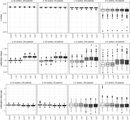
Center‐level c‐statistics, calibration slopes, and calibration intercepts obtained by different models using different sample sizes. The source population used for sampling has an ICC of 20%. The boxplots are made based on the values obtained by fitting and validating the models 500 times. FELR, fixed effects logistic regression; C.RI, random intercept logistic regression using center‐specific random effects; A.RI, random intercept logistic regression assuming average random intercept; M.RI, random intercept logistic regression integrating over the random effect; GEE, generalized estimating equations; SLR, standard logistic regression

Using samples of size 10,000 (50 × 200) for model development should prevent statistical overfitting and hence, a perfect calibration slope of 1 was expected. However, the median calibration slopes obtained by the marginal models were slightly greater than 1, indicating the predicted probabilities were not extreme enough (Figure 1). This is typical for marginal predictions evaluated at the center level (Wynants et al., 2018). In contrast, the conditional predictions were well calibrated on the center level. In case of 50 centers and 50 patients per center, the FELR resulted in a calibration slope slightly smaller than 1 yielding predicted probabilities that were too extreme. This is likely because many center effects need to be estimated and there is not a lot of information to do so. Further, in contrast to RILR, FELR does not use shrinkage of center effects (Snijders & Bosker, 2012).

Development samples with 50 centers and number of patients per center drawn from a Poisson distribution with lambda 50 led to very similar results as those with 50 centers and 50 patients per center (see Supporting Information Figure C.2).

Decreasing the sample size leads to overfitting, which lowers calibration slopes for all models. As a result, when the sample sizes were small (5 × 50), marginal model predictions led to calibration slopes close to 1. The overfitting hence masks the disadvantageous effect of marginal models on the calibration slope.

Models making conditional predictions led to adequate calibration intercepts. Marginal models tended to yield slightly negative calibration intercepts (Figure 1), suggesting some overestimation of predicted risks.

Within each simulation, the center‐level results are averaged over the centers. Hence, results about heterogeneity in performance between centers had to be evaluated as well. The average estimated between‐center variance in calibration slopes was negligible for all types of predictions and sample sizes (<0.0003; Table 4). In case of a development sample of size 10,000 (50 × 200), the average estimated between‐center variance of the calibration intercepts was lowest for the conditional predictions based on the random intercept or fixed effects model (0.67; Table 4). The lower variance for conditional predictions was expected, since center‐specific predictions could be used for centers included in the development set. When there were only five centers in the development sample, the conditional predictions no longer led to a reduction in variance compared to the other predictions.

Table 4.

Average between‐center variance in calibration slope and intercept for all simulation conditions

Average between‐center variance in calibration slope					Average between‐center variance in calibration intercept
	50 centers, 200 patients	50 centers, 50 patients	5 centers, 200 patients	5 centers, 50 patients		50 centers, 200 patients	50 centers, 50 patients	5 centers, 200 patients	5 centers, 50 patients
ICC 5%					ICC 5%
FELR	0.000116	0.000085	0.000115	0.000111	FELR	0.150412	0.177106	0.186903	0.208066
C.RI	0.000122	0.000115	0.000117	0.000116	C.RI	0.148607	0.159240	0.185964	0.202366
A.RI	0.000140	0.000126	0.000117	0.000117	A.RI	0.183680	0.185150	0.188629	0.204069
M.RI	0.000128	0.000113	0.000110	0.000116	M.RI	0.178831	0.180260	0.184730	0.198751
GEE	0.000150	0.000134	0.000124	0.000122	GEE	0.178861	0.180328	0.184637	0.198974
SLR	0.000151	0.000134	0.000125	0.000121	SLR	0.178940	0.180433	0.184862	0.199143
ICC 20%					ICC 20%
FELR	0.000077	0.000286	0.000075	0.000109	FELR	0.674014	0.750286	0.881381	0.972753
C.RI	0.000079	0.000074	0.000076	0.000096	C.RI	0.670376	0.691240	0.877074	0.943464
A.RI	0.000092	0.000079	0.000077	0.000097	A.RI	0.873327	0.878462	0.893019	0.958137
M.RI	0.000030	0.000021	0.000046	0.000106	M.RI	0.790956	0.795093	0.826034	0.874434
GEE	0.000122	0.000104	0.000098	0.000126	GEE	0.788471	0.794514	0.822628	0.872537
SLR	0.000124	0.000106	0.000100	0.000129	SLR	0.791373	0.796660	0.826182	0.879553

	Uniform	Extreme value	Random slope	Dependency		Uniform	Extreme value	Random slope	Dependency
FELR	0.000495	0.000191	0.092956	0.013896	FELR	0.637479	0.642016	0.631857	1.315885
C.RI	0.000506	0.000194	0.094201	0.014242	C.RI	0.634314	0.638339	0.628595	1.283717
A.RI	0.000511	0.000200	0.094578	0.009999	A.RI	0.824441	0.827155	0.817809	1.679083
M.RI	0.000742	0.000564	0.126408	0.015162	M.RI	0.749575	0.753922	0.745689	1.463101
GEE	0.000679	0.000269	0.124778	0.017505	GEE	0.747183	0.748578	0.746005	1.380622
SLR	0.000665	0.000274	0.124797	0.014860	SLR	0.751348	0.745451	0.747522	1.236863
FELR2			0.070592		FELR2			0.676374
C.RS			0.072043		C.RS			0.665660
A.RS			0.087735		A.RS			0.865532
PMM				0.014343	PMM				1.286822
C.PMM				0.014412	C.PMM				1.281027

Abbreviations: FELR, fixed effects logistic regression; C.RI, random intercept logistic regression using center‐specific random effects; A.RI, random intercept logistic regression assuming average random intercept; M.RI, random intercept logistic regression integrating over the random effect; GEE, generalized estimating equations; SLR, standard logistic regression; FELR2, fixed effects logistic regression including center‐predictor interactions; C.RS, random slope logistic regression using center‐specific random effects; A.RS, random slope logistic regression assuming average random effects; PMM, random intercept logistic regression with poor man's method for X1 and X5 assuming average random intercept; C.PMM, random intercept logistic regression with poor man's method for X1 and X5 using center‐specific random effects.

The same patterns for the c‐statistic, calibration slope, and intercept were observed when the ICC was 5%, but the differences between the conditional and the marginal models were less pronounced (see Supporting Information Figure C.3).

4.2. Violation of the normality assumption

When the center effects followed a uniform or extreme value distribution, the c‐statistics, calibration slopes, and calibration intercepts were very similar for all conditional models (Figure 2). As before, the marginal models showed miscalibration.

Figure 2.

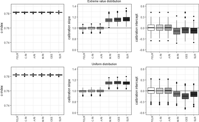
Center‐level c‐statistic, calibration slope, and calibration intercept for the different models in case of a uniform and extreme value random effects distribution. FELR, fixed effects logistic regression; C.RI, random intercept logistic regression using center‐specific random effects; A.RI, random intercept logistic regression assuming average random intercept; M.RI, random intercept logistic regression integrating over the random effect; GEE, generalized estimating equations; SLR, standard logistic regression

Average estimated variances of the slopes were very small for all models (uniform: <0.00075; extreme value: <0.0006). The average estimated variance of the intercepts were smallest for the conditional predictions based on the fixed effects logistic regression and random intercept model using the estimated random effects (0.63–0.64) (Table 4).

These results were very similar to the basic simulation results, indicating that in the context of risk prediction the random intercept model is robust against violations of the normality assumption.

4.3. Center‐predictor interaction (“random slope”)

Ignoring the presence of a center‐predictor interaction only affected the calibration slope (Figure 3). All models ignoring the interaction produced predicted probabilities that were too close to the overall prevalence (FELR, C.RI, A.RI, M.RI, GEE, SLR: slope > 1), but miscalibration was worse for the marginal models.

Figure 3.

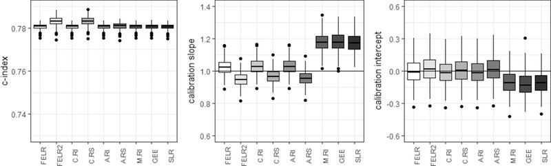
Center‐level c‐statistic, calibration slope, and calibration intercept for the different models in case there is a center‐predictor interaction present in the source populations. FELR, fixed effects logistic regression; FELR2, fixed effects logistic regression including center‐predictor interactions; C.RI, random intercept logistic regression using center‐specific random effects; C.RS, random slope logistic regression using center‐specific random effects; A.RI, random intercept logistic regression assuming average random intercept; A.RS, random slope logistic regression assuming average random effects; M.RI, random intercept logistic regression integrating over the random effect; GEE, generalized estimating equations; SLR, standard logistic regression

When taking into account the center‐predictor interaction by including a random slope in the random effects model (C.RS) or by including interaction terms in the fixed effects model (FELR2), the C‐index could be improved (Figure 3). However, median calibration slopes were below 1, indicating the predicted probabilities were too extreme. (In case validation was performed on new patients from the same centers as in the development phase, the conditional predictions were calibrated.)

Including center‐predictor interactions in the model led to improved between‐center variance in calibration slopes for FELR2 and C.RS compared to FELR and C.RI (0.07 vs. 0.09), but not in calibration intercepts (0.67–0.68 vs. 0.63, Table 4). As before, between‐center differences in calibration were smallest for the conditional predictions based on the fixed effects logistic regression and the random intercept model (Table 4).

4.4. Dependence between center effect and predictors

A dependence between the center effects and predictors is likely to occur when the distribution of predictors varies across centers, for example, due to referral patterns: when nondiseased patients with risk factors indicative for disease are frequently send to specialized centers with a high disease prevalence. In this situation, a random effects model cannot disentangle the within‐center effect (presence of a risk factor in a patient increases this individual's probability of disease) and between‐center effect (centers with a high prevalence also see a lot of patients with the risk factor, but not necessarily the disease). According to Meisner et al. (2017), random intercept models are inadequate under these circumstances in the context of biomarker studies.

SLR had the lowest C‐index (Figure 4). The calibration slopes were slightly below 1 for conditional models and above 1 for marginal models, except for SLR. In contrast to other marginal models, the estimated predictor effects in SLR absorbed part of the between‐center differences, resulting in inflated effect estimates and consequently predicted probabilities that were too extreme. As before, the conditional models yielded calibration intercepts around 0 while the marginal models were miscalibrated.

Figure 4.

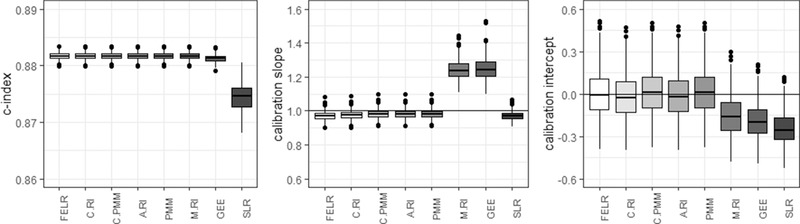
Center‐level c‐statistic, calibration slope, and calibration intercept for the different models in case there is a dependence between the random intercept and predictors X1 and X5 present in the source populations. FELR, fixed effects logistic regression; C.RI, random intercept logistic regression using center‐specific random effects; C.PMM, random intercept logistic regression with poor man's method for X1 and X5 using center‐specific random effects; A.RI, random intercept logistic regression assuming average random intercept; PMM, random intercept logistic regression with poor man's method for X1 and X5 assuming average random intercept; M.RI, random intercept logistic regression integrating over the random effect; GEE, generalized estimating equations; SLR, standard logistic regression

The poor man's method can be used to deal with the correlation between the random intercept and the predictors (Meisner et al., 2017; Neuhaus & Kalbfleisch, 1998). In the current study, these models did not improve calibration much.

The poor man's method was also employed in the calibration models used to calculate calibration intercepts and slopes. Not using PMM in the calibration model led to very similar results.

4.5. Validation results on the population level

In the supporting information file, the population level validation results are presented (see Supporting Information Figures C.4–C.9). Conditional models that use the center‐specific effects (fixed effects logistic regression and random intercept model) resulted in better discrimination compared to other models on the population level. Marginal models were well calibrated on the population level. Conditional predictions were not calibrated on the population level but resulted in calibration slopes below 1 and calibration intercepts above 0. However, conditional predictions based on the random intercept model would be calibrated if for all centers an estimate for the center effect was available (Wynants et al., 2018).

5. DISCUSSION

We investigated the predictive performance of standard logistic regression, generalized estimating equations, fixed effects logistic regression, and random intercept logistic regression using simulations, in which the size of the development sample was varied or some key assumptions underlying the random intercept model were violated. The fixed effects logistic regression and random intercept logistic regression make predictions conditional on the center, the standard logistic regression, generalized estimating equations, and random intercept logistic regression integrating over the random effects make marginal predictions over the centers.

The results of the simulation study show that conditional models are preferable, especially when there are substantial differences between centers. The practical implications of our findings are summarized in Box 1. By using conditional models, systematic over‐ or underestimated predicted risks are avoided. Marginal models yield predictions that are too moderate, too close to the marginal prevalence: this means that in the average center, high risks are underestimated and low risks are overestimated. This is in line with earlier research of Wynants et al. (2018) who compared the predictive performance of a random intercept model and a standard logistic regression model. On top of the models included in this study of Wynants et al. (2018), the current study investigated the predictive performance of fixed effects logistic regression and generalized estimating equations.

Box 1 Recommendations for building prediction models in multicenter data

Marginal or conditional models for multicenter prediction

Use random intercept logistic regression or fixed effects logistic regression with center dummies to obtain good within‐center calibration and overall discrimination, especially when the differences between centers are large.

• Performance is robust to violations of model assumptions and always superior to standard logistic regression or GEE.

• Performance in new centers (using the average intercept) is also superior to standard logistic regression and GEE.

Center dummies or random intercepts

• When there are many centers with few patients, random intercept logistic regression performs slightly better than fixed effects logistic regression.

• Making predictions for new centers has better theoretical underpinning for random intercept regression than for fixed effects regression.

How to use the model to make predictions in new centers?

In absence of information on the new center, use predictions with random intercept 0 to obtain the best expected within‐center calibration. If prevalence estimates or data are available, use existing techniques to tailor the intercept and improve calibration (see, e.g., Debray, Moons, Ahmed, Koffijberg, & Riley, 2013; Steyerberg, 2009; Strobl et al., 2015).

The fixed effects logistic regression and the random intercept model perform very similarly. The fixed effect logistic regression does not perform better than a random intercept model in case of few centers. Only when there are many centers and few patients per center, the fixed effects model performs slightly worse than the random intercept model. Previous research by Kahan (2014) also illustrated using fixed effects logistic regression might introduce bias in the estimated regression coefficients when there are many centers.

A disadvantage of conditional models is that there is no intercept estimate available for centers not included in the development set. The random intercept model provides an intercept for the average center (random intercept set to 0). In contrast, the fixed effects model does not yield an average intercept. In this study, we used the average of all center‐specific intercepts for individuals in new centers.

Although using random effects models leads to satisfactory center‐level performance on average, there may be variability in performance between individual centers. The use of updating methods can be useful to optimally adjust the model to a specific setting (Debray et al., 2013; Steyerberg, 2009; Strobl et al., 2015). Debray et al. (2013) proposed updating methods for random intercept models that do not require data from the new setting. Further research should point out which updating methods work best for multilevel models. Nonetheless, this study demonstrates that using the average center effects yields better predictions in new centers than using a marginal model.

We showed that a small violation of the normality assumption for the distribution of random intercepts should not raise concern when using a random effect model for risk predictions. As a result, random intercept models can lead to reliable predictions to assist medical practitioners in making treatment decisions even when the assumption of normality is not met. This is in line with previous research that suggests random effects models are quite robust against violations of the normality assumption when it comes to estimating the fixed effects (Kahan & Morris, 2013; Maas & Hox, 2004; Neuhaus, Mcculloch, & Boylan, 2013). The current research suggests this is also true within the context of prediction, where the random intercept estimates are of interest to obtain center‐specific prediction. Ignoring the existence of a center‐predictor interaction influenced the predictive performance only minimally in the current simulation.

In reality, the distribution of predictors may differ from center to center. This could give rise to confounding by center. Meisner et al. (2017) illustrated that in the context of biomarker studies a random effects model is inadequate under these circumstances in case of many centers (500) and a negative correlation of −0.5. They found a slight disadvantage of random intercept logistic regression compared to conditional logistic regression in terms of within‐center discrimination and suggest using conditional logistic regression. The regression coefficient estimates of conditional logistic regression are equivalent to those of fixed effects logistic regression. The current research, with positive correlations of 0.5 (continuous predictor and center effects) and 0.2 (dichotomous predictor and center effects) and 50 centers, indicates that in clinical risk prediction a random intercept model yields predictions with good discriminatory performance and only slight miscalibration even when there is a dependency between the center effects and predictors. Further, the fixed effects and random intercept model lead to better predictions than the marginal models, even though the effect of the center and the predictor cannot be distinguished properly. However, it is advisable to remain careful and compare results from a fixed effects (or conditional) logistic regression and a random intercept model.

A strength of the current research is the focus on the performance within each center, which is of interest to clinicians when making predictions for patients in their center. The population level results are also investigated and illustrate that the fixed effects logistic regression and random intercept model result in superior discrimination on the population level. Another strength is that in the simulation study, the validation set includes both centers included in the development set and new centers. This mimics reality and gives a more honest appreciation of the benefit of having center‐specific intercept estimates. In contrast to previous research on random intercept models for prediction (Wynants et al., 2018), the current study investigates the consequences of violating the model assumptions.

A limitation is that we only provided estimates of the center‐to‐center variation for calibration. For the within‐center c‐statistic, we used the estimate proposed by Van Oirbeek and Lesaffre (2012), which does not automatically yield variance estimates. However, there are other measures for the discriminatory performance that do provide an estimate for the center‐to‐center variability (Riley et al., 2015; Snell, Ensor, Debray, Moons, & Riley, 2018; Van Klaveren et al., 2014).

6. CONCLUSIONS

In multicenter prediction research, the multicenter nature of the data is often ignored. The current research illustrates calibration of random intercept logistic regression or fixed effects logistic regression was better than that of standard logistic regression. This is true even when center‐specific intercepts were not normally distributed, a center‐predictor interaction was present, center effects and predictors were dependent, or when the model was applied in a new center. Therefore, we recommend the use of a random intercept model or a fixed effects logistic regression model. The advantage of a random intercept model is that predictions for new centers can easily be made by assuming an average random intercept.

CONFLICT OF INTEREST

The authors have declared that there is no conflict of interest.

Open Research Badges

This article has earned an Open Data badge for making publicly available the digitally‐shareable data necessary to reproduce the reported results. The data is available in the Supporting Information section.

This article has earned an open data badge “Reproducible Research” for making publicly available the code necessary to reproduce the reported results. The results reported in this article were reproduced partially due to data confidentiality issues.

Supporting information

Supporting Information

Supporting Information

Supporting Information

Falconieri N, Van Calster B, Timmerman D, Wynants L. Developing risk models for multicenter data using standard logistic regression produced suboptimal predictions: A simulation study. Biometrical Journal. 2020;62:932–944. 10.1002/bimj.201900075

REFERENCES

- Bouwmeester, W. , Twisk, J. W. , Kappen, T. H. , Van Klei, W. A. , Moons, K. G. , & Vergouwe, Y. (2013). Prediction models for clustered data: Comparison of a random intercept and standard regression model. BMC Medical Research Methodology, 13, 1471–2288. [DOI] [PMC free article] [PubMed] [Google Scholar]
- Debray, T. P. A. , Moons, K. G. M. , Ahmed, I. , Koffijberg, H. , & Riley, R. D. (2013). A framework for developing, implementing, and evaluating clinical prediction models in an individual participant data meta‐analysis. Statistics in Medicine, 32, 3158–3180. [DOI] [PubMed] [Google Scholar]
- Kahan, B. C. (2014). Accounting for centre‐effects in multicentre trials with a binary outcome—When, why, and how? BMC Medical Research Methodology, 14, 1–11. [DOI] [PMC free article] [PubMed] [Google Scholar]
- Kahan, B. C. , & Harhay, M. O. (2015). Many multicenter trials had few events per center, requiring analysis via random‐effects models or GEEs. Journal of Clinical Epidemiology, 68, 1504–1511. [DOI] [PMC free article] [PubMed] [Google Scholar]
- Kahan, B. C. , & Morris, T. P. (2013). Analysis of multicentre trials with continuous outcomes: When and how should we account for centre effects? Statistics in Medicine, 32, 1136–1149. [DOI] [PubMed] [Google Scholar]
- Maas, C. J. M. , & Hox, J. J. (2004). The influence of violations of assumptions on multilevel parameter estimates and their standard errors. Computational Statistics and Data Analysis, 46, 427–440. [Google Scholar]
- Meisner, A. , Parikh, C. R. , & Kerr, K. F. (2017). Biomarker combinations for diagnosis and prognosis in multicenter studies: Principles and methods. Statistical Methods in Medical Research, 1–17. http://journals.sagepub.com/doi/10.1177/0962280217740392 [DOI] [PMC free article] [PubMed] [Google Scholar]
- Moineddin, R. , Matheson, F. I. , & Glazier, R. H. (2007). A simulation study of sample size for multilevel logistic regression models. BMC Medical Research Methodology, 7, 1–10. [DOI] [PMC free article] [PubMed] [Google Scholar]
- Neuhaus, J. M. (1992). Statistical methods for longitudinal and clustered designs with binary responses. Statistical Methods in Medical Research, 1, 249–273. [DOI] [PubMed] [Google Scholar]
- Neuhaus, J. M. , & Kalbfleisch, J. D. (1998). Between‐ and within‐cluster covariate effects in the analysis of clustered data. Biometrics, 54, 638–645. [PubMed] [Google Scholar]
- Neuhaus, J. M. , Mcculloch, C. E. , & Boylan, R. (2013). Estimation of covariate effects in generalized linear mixed models with a misspecified distribution ofrandom intercepts and slopes. Statistics in Medicine, 32, 2419–2429. [DOI] [PubMed] [Google Scholar]
- Pavlou, M. , Ambler, G. , Seaman, S. , & Omar, R. Z. (2015). A note on obtaining correct marginal predictions from a random intercepts model for binary outcomes. BMC Medical Research Methodology, 15, 1–6. [DOI] [PMC free article] [PubMed] [Google Scholar]
- Riley, R. D. , Ahmed, I. , Debray, T. P. A. , Willis, B. H. , Noordzij, J. P. , Higgins, J. P. T. , & Deeks, J. J. (2015). Summarising and validating test accuracy results across multiple studies for use in clinical practice. Statistics in Medicine, 34, 2081–2103. [DOI] [PMC free article] [PubMed] [Google Scholar]
- Snell, K. I. E. , Ensor, J. , Debray, T. P. A. , Moons, K. G. M. , & Riley, R. D. (2018). Meta‐analysis of prediction model performance across multiple studies: Which scale helps ensure between‐study normality for the C‐statistic and calibration measures? Statistical Methods in Medical Research, 27, 3505–3522. [DOI] [PMC free article] [PubMed] [Google Scholar]
- Snijders, T. A. B. , & Bosker, R. J. (2012). Multilevel analysis : An introduction to basic and advanced multilevel modeling (2nd ed.). London: SAGE. [Google Scholar]
- Steyerberg, E. (2009). Clinical prediction models : A practical approach to development, validation, and updating. New York, NY: Springer. [Google Scholar]
- Strobl, A. N. , Vickers, A. J. , Van Calster, B. , Steyerberg, E. , Leach, R. J. , Thompson, I. M. , & Ankerst, D. P. (2015). Improving patient prostate cancer risk assessment: Moving from static, globally‐applied to dynamic, practice‐specific risk calculators. Journal of Biomedical Informatics, 56, 87–93. [DOI] [PMC free article] [PubMed] [Google Scholar]
- Testa, A. , Kaijser, J. , Wynants, L. , Fischerova, D. , Van Holsbeke, C. , Franchi, D. , … Timmerman, D. (2014). Strategies to diagnose ovarian cancer: New evidence from phase 3 of the multicentre international IOTA study. British Journal of Cancer, 111, 680–688. [DOI] [PMC free article] [PubMed] [Google Scholar]
- Timmerman, D. , Testa, A. C. , Bourne, T. , Ferrazzi, E. , Ameye, L. , Konstantinovic, M. L. , … Valentin, L. (2005). Logistic regression model to distinguish between the benign and malignant adnexal mass before surgery: A multicenter study by the International Ovarian Tumor Analysis Group. Journal of Clinical Oncology, 23, 8794–8801. [DOI] [PubMed] [Google Scholar]
- Timmerman, D. , Van Calster, B. , Testa, A. C. , Guerriero, S. , Fischerova, D. , Lissoni, A. A. , … Valentin, L. (2010). Ovarian cancer prediction in adnexal masses using ultrasound‐based logistic regression models: A temporal and external validation study by the IOTA group. Ultrasound in Obstetrics and Gynecology, 36, 226–234. [DOI] [PubMed] [Google Scholar]
- Van Calster, B. , Nieboer, D. , Vergouwe, Y. , De Cock, B. , Pencina, M. J. , & Steyerberg, E. W. (2016). A calibration hierarchy for risk models was defined: From utopia to empirical data. Journal of Clinical Epidemiology, 74, 167–176. [DOI] [PubMed] [Google Scholar]
- Van Holsbeke, C. , Van Calster, B. , Testa, A. C. , Domali, E. , Lu, C. , Van Huffel, S. , … Timmerman, D. (2009). Prospective internal validation of mathematical models to predict malignancy in adnexal masses: Results from the international ovarian tumor analysis study. Clinical Cancer Research, 15, 684–691. [DOI] [PubMed] [Google Scholar]
- Van Klaveren, D. , Steyerberg, E. W. , Perel, P. , & Vergouwe, Y. (2014). Assessing discriminative ability of risk models in clustered data. BMC Medical Research Methodology, 14, 1–10. [DOI] [PMC free article] [PubMed] [Google Scholar]
- Van Oirbeek, R. , & Lesaffre, E. (2012). Assessing the predictive ability of a multilevel binary regression model. Computational Statistics and Data Analysis, 56, 1966–1980. [Google Scholar]
- Vergouwe, Y. , Moons, K. G. M. , & Steyerberg, E. W. (2010). External validity of risk models: Use of benchmark values to disentangle a case‐mix effect from incorrect coefficients. American Journal of Epidemiology, 172, 971–980. [DOI] [PMC free article] [PubMed] [Google Scholar]
- Wynants, L. , Kent, D. M. , Timmerman, D. , Lunquist, C. M. , & Van Calster, B. (2019). Untapped potential of multicenter studies: A review of cariovascular risk prediction models revealed inappropriate analyses and wide variation in reporting. Diagnostic and Prognostic Research, 3(1), 6 10.1186/s41512-019-0046-9 [DOI] [PMC free article] [PubMed] [Google Scholar]
- Wynants, L. , Vergouwe, Y. , Van Huffel, S. , Timmerman, D. , & Van Calster, B. (2018). Does ignoring clustering in multicenter data influence the performance of prediction models? A simulation study. Statistical Methods in Medical Research, 27, 1723–1736. [DOI] [PubMed] [Google Scholar]
- Zeger, S. L. , Liang, K.‐Y. , & Albert, P. S. (1988). Models for longitudinal data: A generalized estimating equation approach. Biometrics, 44, 1049–1060. [PubMed] [Google Scholar]
Associated Data
This section collects any data citations, data availability statements, or supplementary materials included in this article.
Supplementary Materials