Predicting protein-protein interactions on a proteome scale by matching evolutionary and structural similarities at interfaces using PRISM

Abstract

Prediction of protein-protein interactions at the structural level on the proteome scale is important because it allows prediction of protein function, helps drug discovery and takes steps toward genome-wide structural systems biology. We provide a protocol (termed PRISM, protein interactions by structural matching) for large-scale prediction of protein-protein interactions and assembly of protein complex structures. The method consists of two components: rigid-body structural comparisons of target proteins to known template protein-protein interfaces and flexible refinement using a docking energy function. The PRISM rationale follows our observation that globally different protein structures can interact via similar architectural motifs. PRISM predicts binding residues by using structural similarity and evolutionary conservation of putative binding residue ‘hot spots’. Ultimately, PRISM could help to construct cellular pathways and functional, proteome-scale annotation. PRISM is implemented in Python and runs in a UNIX environment.

INTRODUCTION

Protein-protein interactions are involved in all in vivo functions: regulation of the cell cycle; degradation; viral entry; metabolic and signal transduction pathways; initiation of DNA replication; all steps in transcription, translation and splicing; enzymatic reactions and their regulation; and the immune response¹. Knowledge of the structural proteome would be immensely useful: it would provide information that is not only related to the proteins that interact, but also to how they interact. Structural data would help in assigning function to proteins and in figuring out functional mechanisms and regulation; in suggesting which proteins can and cannot interact simultaneously, which can help in constructing the cellular pathways; and in drug discovery, which would target particular protein-protein interfaces and minimize side effects in proteins with similar interfaces. It would also help in understanding the dynamics of the cellular network that reflects protein concentrations and the fluctuating environment. Genome-wide prediction of the structural proteome has been a major aim in structural and functional genomics. The problem is, however, that, from the experimental standpoint, such large-scale determination of the structures of multimolecular complexes is highly challenging; from the computational standpoint, this goal is similarly daunting.

Current experimental approaches such as high-throughput mass spectrometry² and the yeast two-hybrid system³ provide a wealth of large-scale protein-protein interaction data that have been organized in protein interaction databases^4,5; X-ray crystallography and NMR provide 3D structures of some of these⁶. These are accompanied by mutational data^7,8, which yield relative binding strengths. Nevertheless, the gap between the available data relating to cellular networks, which suggest which proteins interact, and the structural proteome is immense and widening. Computational methods can assist by addressing protein-protein interactions at different levels: they can predict the binding sites of proteins, find specific residues contributing dominantly to the association and ultimately design specific interfaces. Further, computational ‘docking’ methods^9–16 can predict protein-protein interactions. Docking methods aim to predict the native association of proteins when there are data suggesting that they interact, and when their structures are available. On the plus side, docking models are refined and their energies evaluated. However, even apart from the computational costs, in the absence of additional biochemical data relating to the interaction site, it is very difficult to distinguish between the models and predict the native interaction because there are many energetically favorable ways for proteins to interact. Docking becomes much more challenging and computationally demanding if we want to apply it on the proteome scale when we do not know which proteins interact. An alternative strategy is knowledge based, using stuctural similarity to an interface of a known protein complex.

Protein interface structures are evolutionarily more conserved than other surface regions of the proteins¹⁷. Further, as we have shown, protein pairs with different global structures and different functions can associate via similar interface architectures^18–21. Therefore, the use of interface architectures can generate promising models for protein complexes even in the absence of global sequence or fold similarity. PRISM^22,23 is the first algorithm using this powerful concept to model protein complexes: if two complementary sides of a template interface are structurally similar to the surfaces of two target proteins, then these two proteins can interact with each other using this template interface architecture even if the remainder of the structures are dissimilar. The first version was released as a web server in 2005 (refs. 22,23). It considered only rigid structural similarity. This first version was reviewed in 2008 (ref. 24). PRISM has been used in several studies including comparison of physicochemical properties of cancer-related protein complexes on a large scale²⁵ and understanding time-dependent formation of protein complexes in the p53 pathway²⁶. The method has evolved with our efforts to increase its prediction accuracy. This protocol presents the latest version of PRISM combining for the first time large-scale rigid-body structural alignments with flexible refinement and energy minimization to model protein-protein interactions. It is a powerful combinatorial multiscale strategy toward predicting genome-wide functional associations of the proteome. This new version has been recently used to show case studies on allosteric events in signaling²⁷, relationships between hot spots and conformational selection²⁸ and to predict which interactions can co-occur in the p53 pathway²⁶.

Overview of the PRISM algorithm, its rationale and application to model cellular pathways

A protein-protein interface data set is particularly useful for 3D modeling of protein complexes. This is because the number of naturally occurring architectural motifs—in single-chain proteins and, as we have shown over the years, in protein-protein interfaces—is limited^19,20,29,30. Inspired by this observation, PRISM uses two types of data sets: a template data set composed of protein-protein interface structures derived from the Protein Data Bank (PDB) and a target data set that contains the structures of those protein chains the interactions of which are sought. The default template data set that comes with the protocol is a subset of a structurally nonredundant data set of known protein-protein interfaces³⁰. This data set can be replaced by another template set (see Box 1).

BOX 1 |. CONSTRUCTION OF THE TEMPLATE AND TARGET DATA SETS.

The template data set:

Protein interfaces are represented by six-letter nomenclature; the first four letters correspond to the PDB name and the following two letters are chain identifiers. In other words, the interface between chain A and B of the PDB structure 1c1y is named 1c1yAB. There are several methods to extract the protein interface, e.g., using atomic distances, solvent accessibilities or Voronoi diagrams. In this protocol, the default template set is generated using atomic distances. To extract interfaces, two types of residues in each chain are defined: ‘interacting’ and ‘nearby’. If the distance between any two atoms of two residues, one from each chain, is less than the sum of their van der Waals radii plus a 0.5-Å tolerance, these two residues are flagged as ‘interacting’; if the distance between the C^α of a noninteracting residue and an interacting residue in the same chain is under 6 Å, the noninteracting residue is flagged as a ‘nearby’ residue. For correct matching, the exact architecture of an interface is necessary. The nearby residues are very important for the description of the architecture of the template interfaces. If other methods are used for extracting interfaces, nearby residues must be included. The default template set contains 1,036 structurally nonredundant heterodimeric interfaces.

Using the interfaces in this data set as templates, new potentially interacting protein pairs are predicted. Another template interface set can be used. The default template set is available in 1-Prediction/TEMPLATE/, which contains interfaces and hotspot_data. In the interfaces directory, the C^α atom coordinates of residues of template interfaces are available in PDB format as follows:

ATOM 365 CA ASN A 47 40.814 − 38.861 76.232 1.00 19.70 C 
ATOM 373 CA PRO A 48 42.938 − 35.800 77.060 1.00 18.83 C 
ATOM 380 CA LYS A 49 42.229 − 34.529 73.529 1.00 15.24 C 
ATOM 389 CA GLY A 50 38.451 − 34.398 74.17 1.00 13.35 C 
ATOM 393 CA GLN A 51 37.509 − 35.834 70.798 1.00 13.64 C 
ATOM 402 CA VAL A 52 35.650 − 38.840 69.418 1.00 9.49 C

In the hotspot_data directory, computational hot spots are deposited for each interface in the default template set. In the current version, the HotPoint web server (see Box 2) is used to predict hot spots. The file format is as follows:

# 1a0fAB.pdb 30 30 
A.T.64 T 
A.E.65 E 
A.A.68 A 
A.Q.71 Q 
A.D.75 D 
… 
… 

Here the first line provides the name of the template interface (e.g., 1a0fAB.pdb) and the total number of hot spots (30 30) in that interface. Further, the hot spots are listed. The first column lists the chain identifier, residue name and residue number; in the second column the one-letter residue name is given. For more details of the template interface file formats, users may go over the available template files.

The target data set:

The target set contains proteins for which potential interactions among them are to be predicted. To find if they interact directly, their surfaces will be structurally compared with the template interfaces.

The rationale of PRISM is as follows: if complementary partners of a template interface are similar to surface regions of any two proteins, these two proteins can interact with each other through these regions. When searching for similar spatial motifs on the target protein surface, PRISM considers both geometric complementarity detected by structural alignments and evolutionary conservation of hot spots. No sequence similarity is used. Figure 1 presents a flowchart of the algorithm.

Figure 1 |.

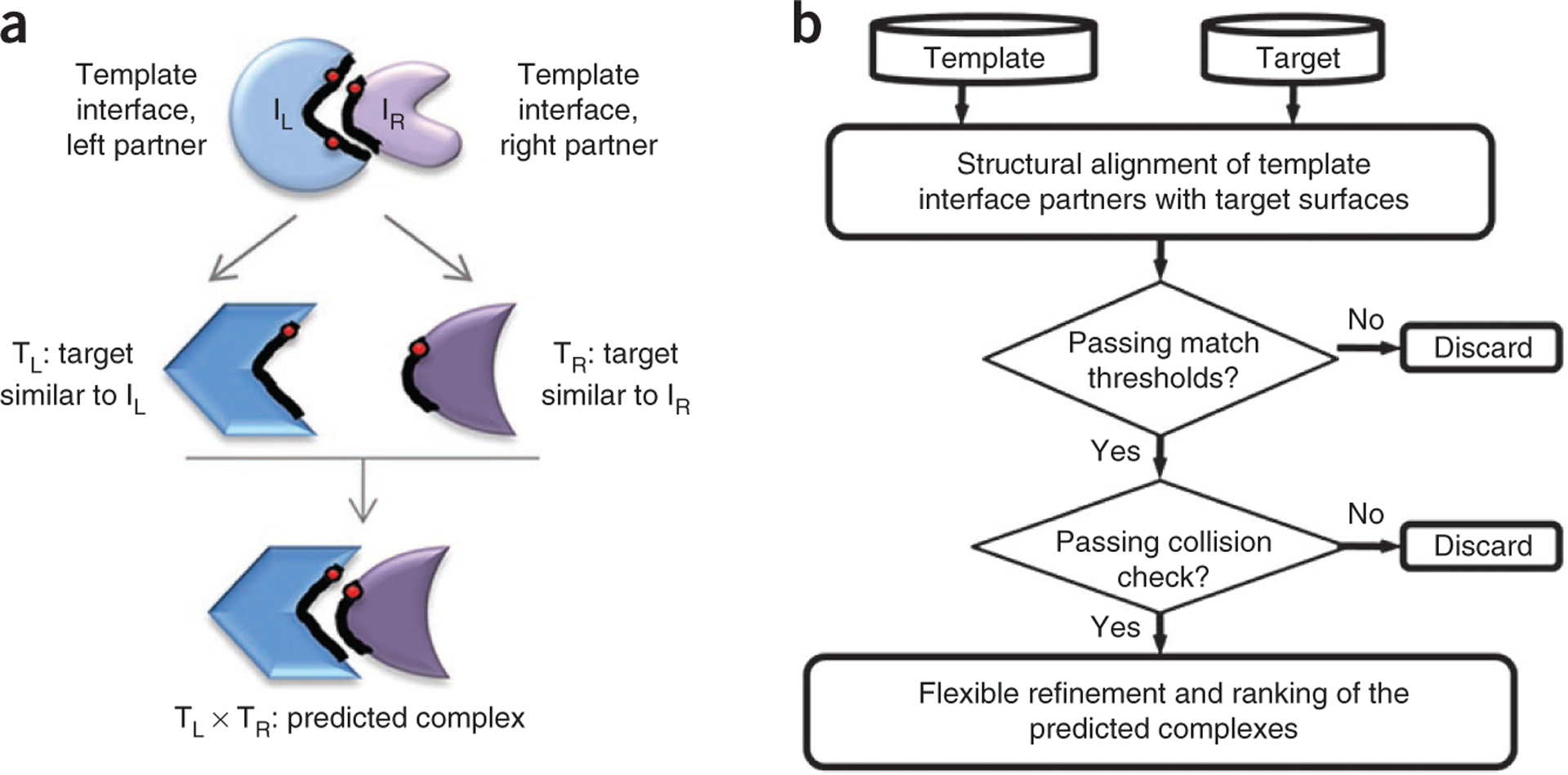
Description of the prediction algorithm. (a) Schematic illustration of the concept of the prediction algorithm. If complementary partners (I_L and I_R) of a template interface are similar to surface regions of any two targets (T_L and T_R), these two targets can interact with each other via these regions. The red points are hot spots. These incorporate evolutionary information into the matching. (b) The flowchart of the algorithm. There are two data sets in the algorithm: the template data set and the target data set. First, the surface of the proteins in the target data set is extracted. Next, each partner of the template interface is aligned with the target surfaces. If the match passes the residue and hot spot matching thresholds, these targets are transformed on the template interface. If there are colliding residues (e.g., atoms of the residues penetrate into each other’s van der Waals radii after they are transformed onto the corresponding template interface) between the two partner targets, the putative complexes are eliminated. Otherwise, the predicted complexes are flexibly refined with their global energies computed. The best solution is chosen as the one with the lowest energy value.

The prediction algorithm is composed of four consecutive phases. Proteins interact through surface residues; thus, in the initial phase, the surface regions of target proteins are extracted. In the second phase, using structural alignments, the similarity of each side of a known interface to monomer surface regions is evaluated. Specifically, each interface in the template data set is split into its constituent chains. Using the MultiProt³¹, our method searches whether the complementary sides of a template interface are structurally similar to any region on the target surfaces. MultiProt searches for spatial residue similarities disregarding the order of the residues on the chain. This is important because interfaces and surfaces often consist of single residues and short fragments that are not contiguous in the protein sequence. In the third phase, the two chains, the surface regions of which are similar to the two parts of the template interface, are transformed onto this template forming a complex structure, and the solution is assessed. The last phase involves flexible refinement of the rigid docking solutions of MultiProt to resolve steric clashes, especially of side chains, and ranking of the putative complexes by the global energy. This is done by using FiberDock³², which calculates energies and ranks the predicted protein complexes according to these. In this way, the geometric complementarity is combined with docking procedures, which makes the method more physical.

Comparison with existing methods

Among the knowledge-based approaches, homology-based prediction methods were the first to be developed. In homology-based methods, sequence or structure homologs of target proteins are searched on template complexes and the interaction is modeled accordingly^33–36. As noted in the previous section, PRISM^22,23 is the first algorithm for protein interaction prediction that uses only interface architectures as templates, independent of global sequence or structure homology, because in nature, similar protein interface architectures are reused by structurally and functionally different protein pairs^19,20,29. Templates of homology-based methods are more restricted because there should be homologous sequences in the template structures. The pure geometry-based strategy of PRISM makes the predictions more diverse. Following PRISM, several other prediction algorithms have also emerged based on a similar concept^37,38. For example, ISearch uses domain interfaces as templates for prediction, and predictions are inferred also solely from rigid-body alignments³⁷. Another method has also shown that local similarities are more accurate in modeling protein complexes³⁸, and that the accuracy of these template-based approaches is sufficient for large-scale predictions³⁹. The differences among these otherwise similar methods stem from the selection of template data sets and from the matching thresholds in the rigid-body alignment stage. When the new version of PRISM is compared with other knowledge-based approaches, the advantage of PRISM comes from its combinatorial procedure that integrates template-based rigid-body alignment with flexible side-chain and backbone refinement. On their own, neither knowledge-based nor docking methods are effective enough to obtain accurate predictions. Using only structural comparison greatly reduces the solution space; however, it disregards flexibility and foregoes energetic assessment. On the other hand, carrying out docking on a database scale is difficult, because of both the computational time limitations and too many high-scoring false solutions. For comparison with the rigid-body docking, we selected Zdock¹⁵ and Pathdock¹⁶. A rigid-body docking of a protein pair using Zdock¹⁵ takes 4 min on 16 processors; using PatchDock^16, it takes less than 10 min on a single processor. Running of all pairs of these N targets takes (N × (N − 1) / 2) × 10 min quadratic running time, in the best case. For a small number of target proteins, all methods have more or less similar running times. As the target data set increases, the difference between the running times of PRISM and such docking programs gets larger and the advantage of a template-based method for large-scale application is obvious. On the plus side, docking solutions are refined and their energies are evaluated. Here, by combining the two approaches, we restrict the solution space and eliminate false positives. Another consequence of reducing the solution space is computational effectiveness, especially on the proteome scale. Nevertheless, there are some limitations when using PRISM: first, PRISM predictions are restricted to available target protein structures; that is, they depend on the coverage of the protein-protein template data set. Therefore, it is crucial to start with a template set that is as complete as possible, so that it covers different types of interface architectures. Because the size and coverage of the PDB increases exponentially, we expect the potential usage of PRISM to increase. Currently, more than 6,000 unique human proteins have structures in PDB, covering ~30% of the known functional classes⁴⁰. Homology modeling and other structure prediction techniques further increase this number. The structural coverage of the human proteome is almost 50% when reliable homology models are also considered⁴¹. The second limitation is that the current version does not handle protein-peptide interactions. PRISM provides the interactions and their atomic details. The first can be validated by checking against protein-protein interaction databases. For atomic details, the results can be compared with those from other binding-site prediction programs^42,43, and ultimately tested by site-directed mutagenesis experiments⁴⁴.

MATERIALS

EQUIPMENT

A computer running in a Unix environment.

EQUIPMENT SETUP

PRISM

PRISM is composed of four consecutive steps. The PRISM scripts are written in the Python language (tested with 2.5.x). The Numpy numeric package for Python must also be installed. A Perl interpreter and Fortran compiler are also needed to run some of the external programs. The PRISM installation guide is illustrated below in the Procedure. The program can be downloaded at http://prism.ccbb.ku.edu.tr/prism_protocol/.

Data format

The coordinates of protein structures or homology models in PDB format are used as target proteins. The coordinates of the structure of template complexes also should be in PDB format (see Box 1).

External tools

PRISM integrates external tools to perform several jobs, i.e., Naccess for calculating solvent accessibility, MultiProt for structural alignment, FASTA (version 35) for sequence alignment and FiberDock (version 1.0) for flexible refinement and scoring of solutions. All of these programs are freely available for academic use.

PROCEDURE

Install PRISM

• 1Set up necessary environment to run PRISM (as detailed in EQUIPMENT SETUP).
• 2
  Download the PRISM source codes at http://prism.ccbb.ku.edu.tr/prism_protocol. Follow the download instructions. Installation of PRISM is a straightforward procedure. Unzip the downloaded PRISM_protocol.tar.gz file and extract it. You may use the command below:

  > tar –xvzf PRISM_protocol.tar.gz 
  

• 3
  Type the following command:

   > cd PRISM_protocol 
  

  This command changes the current directory to the PRISM_protocol directory. Check whether four directories (0-SurfaceExtraction, 1-Prediction, 2-DistanceCalculation, 6-FiberDock) are available in the PRISM_protocol directory.

Install external programs

• 4
  Install external programs by following their installation guides. Follow the instruction of each external program to have the executables. Before the PRISM run, ensure that the external programs and tools are running properly. The links to the pages of external tools are available in the download page of PRISM. These programs should be installed into PRISM_ protocol/EXTERNAL_TOOLS using the following options: option A to install FASTA version 35; option B to install MultiProt; option C to install Naccess; and option D to install FiberDock:

  1. Installing FASTA version 35

     1. FASTA⁴⁵ version 35 is used for sequence alignment to eliminate homologous sequences. Download FASTA version 35 into PRISM_protocol/EXTERNAL_TOOLS.
     2. To install FASTA version 35, change directory to EXTERNAL_TOOLS:

        > cd EXTERNAL_TOOLS
        

     3. Extract the fasta-35.4.12.tar file:

        > tar –xvf fasta-35.4.12.tar
        

     4. Rename the resulting directory as fasta35:

        > mv fasta-35.4.12 fasta35
        

     5. Follow the FASTA installation instructions in the README file under fasta35.
  2. Installing MultiProt

     1. MultiProt³¹ is used to perform structural alignment. Download MultiProt 1.6 into PRISM_protocol/EXTERNAL_ TOOLS.
     2. To install MultiProt, change directory to EXTERNAL_TOOLS:

        > cd EXTERNAL_TOOLS
        

     3. Extract multiprot1.6.tar file:

        > tar –xvf multiprot1.6.tar
        

     4. Rename the resulting directory as multiprot:

        > mv multiprot1.6 multiprot
        

  3. Installing Naccess

     1. Naccess⁴⁶ is used to calculate the accessible surface area of residues. Download Naccess into PRISM_protocol/ EXTERNAL_TOOLS.
     2. To install Naccess, change directory to EXTERNAL_TOOLS:

        > cd EXTERNAL_TOOLS
        

     3. Extract the naccess.tar file:

        > tar –xvf naccess.tar
        

     4. Rename the resulting directory as naccess:

        > mv naccess2.1.1 naccess
        

     5. Follow the installation instructions in the README file under naccess.
        ▲ CRITICAL STEP Note that the installation script uses f77 (fortran compiler); please follow the Naccess installation instructions.
     ? TROUBLESHOOTING
  4. Installing FiberDock

     1. FiberDock³² is used for flexible refinement and for scoring the solutions with an empirical energy function. Download FiberDock version 1.0 into PRISM_protocol/EXTERNAL_TOOLS.
     2. To install FiberDock, change directory to EXTERNAL_TOOLS:

        cd EXTERNAL_TOOLS
        

     3. Unzip the fiber_dock_download.v1.zip file:

        > unzip fiber_dock_download.v1.zip
        

     4. Rename the resulting directory as fiberdock:

        > mv FiberDock1.0 fiberdock
        

        ▲ CRITICAL STEP Note that the default FiberDock executable is for 64-bit machines. For 32-bit machines, you have to download FiberDock1.1 and rename FiberDock.32 as FiberDock.

Prepare the data sets

• 5
  Decide which template set you would like to use—follow option A to use the default template set or option B to use a customized template set.

  1. Using the default template set

     1. A user can work with the default template set supplied in the PRISM installation package. The default template set is available in PRISM_protocol/1-Prediction/TEMPLATE.
  2. Constructing a new template data set

     1. (Optional) If the user does not wish to use the default template set and instead prefers to use a customized template set specific to the scientific problem, she/he needs to construct a new template data set. To do this, first prepare the C^α atom coordinates of the interface residues in PDB format (the data format guide is available in Box 1). For this step, we provide a Python script (in the PRISM_protocol/OPTIONAL_TemplatePrepare directory), which prepares the coordinates of the interface residues in PDB format based on the distance thresholds mentioned in Box 1. To run the script templateGenerator.py, change the current directory to the PRISM_protocol/OPTIONAL_ TemplatePrepare/ as follows:

        > cd PRISM_protocol/OPTIONAL_TemplatePrepare/
        

     2. Transfer the corresponding PDB complex file of the template interfaces into the PDB directory here.
     3. Run the templateGenerate.py script as follows, where interfaceID = six-letter name of the template interface (see Box 1) and pdbpath = the full path where corresponding pdb complex files of all template interfaces are located:

        > python templateGenerator.py [interfaceID] [pdbpath]
        

     4. Extract hot spot residues and prepare hot spot files in the format as described in Box 1 (also, see Box 2).
     5. Substitute the TEMPLATE directory in PRISM_protocol/1-Prediction with the new set generated here.
• 6
  Prepare the list of target proteins (to see the description of target set, refer to Box 1) by listing the PDB names of the target proteins in the file named PDB. list in PRISM_protocol/0-SurfaceExtraction directory; i.e.,

  1F51 
  2C2A 
  1PEY 
  …
  …
  

• 7
  Download the protein structures listed in PDB.list manually using option A or automatically from the PDB ftp site using option B. For structures that are not available in PDB, use option C:

  1. Manual downloading

     1. To manually download the target structures, browse to the PDB web page (http://www.pdb.org) and download the corresponding structures.
     2. The full path of the directory containing the pdb files will be needed later while running PRISM.
  2. Automatically downloading

     1. To automatically download the target structures, run the python script PDBdownload.py in PRISM_protocol/0-SurfaceExtraction directory. To run this script, just type the following command:

        > python PDBdownload.py
        

     It will download all pdb structures in your PDB.list file and deposit them into the PRISM_protocol/0-SurfaceExtraction/PDB directory. This script needs an Internet connection.
  3. Using structures that are not available in PDB

     1. If a protein structure does not have a PDB ID (e.g., homology models), provide a four-letter artificial ID, i.e., 1111 or aaaa, to run the surface extraction algorithm. Moreover, the sequence of the protein should be added to the PDB_ FASTA file in 0-SurfaceExtraction and in 1-Prediction in FASTA format.

BOX 2 |. CRITICAL RESIDUES IN BINDING REGIONS: HOT SPOTS.

The contribution of residues in the binding region of proteins is not uniform; rather they contain critical residues called hot spots⁷. Hot spots are primary targets of therapeutic agents because designing a molecule that will bind to hot spots may lead to the disruption of a protein-protein interaction. Experimentally, hot spots are determined by alanine-scanning mutagenesis in which, if the contribution of the mutated residue to the binding is more than 2.0 kcal mol⁻¹, these residues are labeled as hot spots. Trp, Tyr and Arg are frequently seen as hot spots in protein interfaces because of their sizes. The characteristics of hot spots point out that they are buried in the protein interface, structurally conserved and are surrounded by a rim region composed of ‘less important’ residues. Further, hot spots come together and form tightly packed regions called ‘hot regions’. Keeping in mind their unquestionable role in binding, we use hot spots in prediction of protein-protein interactions, which provide evolutionary insights into the predictions.

In this protocol, we use the HotPoint web server⁴⁸ to predict hot spots in template protein interfaces, which is freely available to all users. HotPoint labels a residue as a hot spot if it is buried (its relative accessibility is less than 20%, as determined by Naccess⁴⁶) and its total contact potential (with respect to its neighbors within a radius of 7.0 Å) is large (more than 18.0). For further details, please see references 48,49. Besides HotPoint, there are several web servers and databases for hot spot prediction. Moreover, there are experimental hot spot data in the literature and in some databases^50,51. As long as the necessary format is used as input data, any available hot spot data can be used for prediction (see Box 1).

Surface extraction of target proteins

• 8
  After preparation of template and target data sets and proper installation of PRISM, it can be run by executing command-line python scripts. If PRISM is installed in the /home/project/PRISM_protocol directory, change the current directory to the PRISM_protocol/0-SurfaceExtraction:

  > cd/home/project/PRISM_protocol/0-SurfaceExtraction
  

• 9Transfer the PDB.list file into the directory 0-SurfaceExtraction.
• 10
  Run surfaceExtractor.py using the following command-line script, where pdbpath = the full path in which pdb files of all target proteins are located, workpath = the full path in which you are running surfaceExtractor.py, target_startindex = target protein index to start and target_endindex = target protein index to end:

  > python surfaceExtractor.py [pdbpath] [workpath] target_startindex target_endindex Target protein indices come from the order in PDB.list file. Pay attention to give the full path of [pdbpath] and [workpath]. If there are 50 target proteins to be considered in the surface extraction step, the startindex is 1 and endindex is 50. For example: Python surfaceExtractor.py/home/project/PRISM_protocol/0-SurfaceExtraction/PDB/home/ project/PRISM_protocol/0-SurfaceExtraction 1 50
  

  The surfaceExtractor.py code in 0-SurfaceExtraction directory performs all the steps described in Box 3.

  ? TROUBLESHOOTING

• 11Check 0-SurfaceExtraction/TARGET_SURFACES directory. It contains the *.asa.map, *.asa.pdb files. *.asa.map files contain the names of surface residues and their nearby residues. *.asa.pdb files contain the coordinates of the residues of target surface shell in PDB format. There should be a file called 0-SurfaceExtraction/ all_pdbs.paths that contains the file paths of the surface files that are required for the next step.

BOX 3 |. STEPS PERFORMED BY THE PROGRAM.

1. Steps/functions performed by the surfaceExtractor.py code

   1. Checks whether the target protein is a monomer or a multimer. If the target is a multimeric protein, it is divided into its constituent chains.
   2. Checks whether the target chains contain DNA or RNA structures. DNA and RNA structures are not considered in the prediction algorithm.
   3. Checks the homology of the constituent chains of the target proteins.
   4. To name the surface of each chain, the four-letter pdb name is followed by the identifiers of homologous chains; i.e., chains A, C and E are homologous in 1axc protein; thus, to avoid redundancy, chain A is represented as 1axcACE.
   5. Runs Naccess for each target protein chain. Naccess rolls a solvent probe on the desired molecule. The radius of the solvent can be chosen by the user, but the default value is 1.4 Å. The path gained by the center of the probe gives the accessible surface area.
   6. Extracts surface residues of target proteins. Protein ‘surface’ is the shell around the entire monomer surface. The surface regions in the target data set are extracted based on the relative accessible surface area of the residues. If the relative accessibility (accessible surface area versus that of the residue in an extended conformation) of a residue is more than 15% (the default value), it is labeled as a surface residue. The default value can be modified (the parameter RSATHRESHOLD in surfaceExtractor.py).
   7. Extracts nearby residues of surface residues. Nearby residues are used to provide the structural scaffolds of the protein surfaces. A residue is defined as ‘nearby’ if the distance between its C^α atom and that of a surface residue is under 5.0 Å. Nearby residues are important in the structural alignment phase. The default parameter is 5.0 Å. It can be modified for individual runs (the parameter SCFFTHRESHOLD in surfaceExtractor.py).
2. Steps performed by structuralAlignment.py

   1. Split each template interface into its two complementary partners.
   2. Align structurally each partner of the template interface with the target surfaces using the MultiProt engine. For a brief description of the MultiProt algorithm, please refer to Box 4. The 1-Prediction/params.txt contains the parameters for structural alignment:

      • The SeqOrder parameter is set to 0 for sequence order–independent matching. MultiProt searches for spatial similarities of aa coordinates disregarding the order of the residues on the chain. Because template interfaces and target surfaces do not consist of contiguous chains, MultiProt is particularly appropriate for our interface-to-surface comparison.
      • For each individual alignment, MultiProt reports the ten best substructural matches. The number of solutions can be changed using the parameter ResNum.
      • Matching is strict: maximal RMSD is 2.0 Å with minimal match size set to five residues. The maximal RMSD for matching two rigid fragments is defined by the parameter SeqBlockRMSDthr. The parameter for minimal size of rigidly matched fragments is SeqBlockMinSize. The default values 2.0 and 5 are changeable if a more relaxed structural matching is necessary.
      • OnlyRefMol is set to 0 in order not to restrict the reference structure to the first molecule in the alignment; in this way the best match between two structures is obtained.
      • Geometry and residue type (hydrophobic, hydrophilic, aromatic or glycine) are considered in the structural alignment by setting Scoring to 2 and Biocore to 3. If the user wants to use pure geometry for alignment, Scoring should be set to 0.
   3. Matching solutions are deposited in the MULTIPROT_OUTPUT folder. For each template interface, a folder is created with six-letter naming of protein interfaces. The naming is as follows:

      templateName/templateName_templateChain_targetName_2_sol.res. For example, the file 1c1yAB/ 1c1yAB_A_1ycsA_2_sol.res is the solution file of the matching between chain A of the target 1ycs and chain A of the template 1c1yAB.
      

3. Steps performed by the TransformationFiltering.py code

   1. Check the structural matching thresholds.

      • A total of 50% of the residues of template chains should geometrically match the target surfaces to pass to the next step (see the parameter MINIMUM_RESIDUE_MATCH_PERCENTAGE). This threshold is 30% for template chains containing more than 50 residues (the parameter DIFF_PERCENTAGE can be used to change the difference between thresholds for small template interfaces and large template interfaces. Its default value is 20.). In both cases, the number of matching residues should be at least 15 (see the parameter MINIMUM_RESIDUE_MATCH_COUNT).
      • At least one hot spot in each template partner should correctly match with the target surface (see the parameter MINIMUM_ HOTSPOT_MATCH_NUMBER). Hot spot filtering incorporates evolutionary similarity between target surface and template interface in addition to structural similarity.
   2. Transform target proteins on their similar template interface to form the complex sructure. MultiProt solution files contain the transformation matrix for each matching. Using these matrices, each target protein is transformed onto the corresponding template interface partner. Transformations are applied to the entire target structure, not only to the surface region.
   3. Check colliding residues after transformation. If two partners have (more than five) spatially colliding residues, the match is eliminated. Side-chain clashes are not considered at this stage. A more rigorous refinement is performed at the last phase of the algorithm.
   4. Check whether complementary partners of the matching residues of the template interface are in contact. Sometimes, especially in large template interfaces, matching residues in the left and right partners are not against each other. To guarantee the correct matching, there should be at least five contacts between matching residues of the complementary partners of the template interface.
4. Steps performed by the FlexibleRefinement.py code

   1. Add hydrogens to the transformed target proteins.
   2. The backbone flexibility is modeled by normal modes. Calculate normal modes of each chain of the putative complex coming from the previous part. Here the first 50 modes of each protein are considered.
   3. Prepare the parameter file.

      • Select the larger protein chain (in size) as the receptor molecule and the smaller one as the ligand.
      • Select the restricted side-chain optimization option where only clashing interface residues are assumed to be movable at both receptor and ligand site.
      • A total of 20% of the clashes between the side-chain atoms are allowed by setting the atomic radius scale parameter to 0.8.
      • Because we already transformed the target proteins onto template interfaces, here the zero-transformation matrix is used for energy calculation, which is given in the zero-transformation file.
   4. Run FiberDock to calculate the binding energy and to optimize the predicted protein complex. For side-chain flexibility, it uses a rotamer library and finds optimum combination of rotamers with the lowest total energy. At each iteration, normal modes with a high correlation to the repulsive van der Waals forces are considered and applied to the flexible protein. High correlation implies that the directions of the force vectors and normal modes are similar. Finally, FiberDock calculates energies. For energy calculations, the CHARMM⁵² force field is used.

Structural matching of targets with templates

• 12
  Change the current directory to the PRISM_protocol/1-Prediction as follows:

  > cd/home/project/PRISM_protocol/1-Prediction
  

• 13
  Copy the all_pdbs.paths file created in the previous step into the PATHS directory:

  > cp ../0-SurfaceExtraction/all_pdbs.paths PATHS
  

• 14
  Run the command below, where [templatePath] = the full path in which your template files are deposited, [workpath] = the full path in which you are running structuralAlignment.py, startindex = template interface index to start and endindex = template interface index to end:

   > python structuralAlignment.py [templatePath] [workpath] startindex endindex These indices (startindex and endindex) are based on the order of ‘ls’ command of the templates. The default template set contains 1,036 interfaces. Pay attention to give the full path of [templatePath] and [workpath]. For example:
  > python structuralAlignment.py/home/project/PRISM_protocol/1-Prediction/TEMPLATE/ home/project/PRISM_protocol/1-Prediction 1 1036
  

  The structuralAlignment.py code in the 1-Prediction directory performs all the steps as explained in Box 3. For details of the MultiProt program, refer to Box 4.

• 15Check the 1-Prediction/MULTIPROT_OUTPUT directory. It contains the MultiProt results files arranged in directories labeled by template interfaces.

BOX 4 |. DETAILS OF STRUCTURAL ALIGNMENT AND FLEXIBLE REFINEMENT.

The MultiProt algorithm

PRISM uses the MultiProt engine as an external program to perform structural alignment. MultiProt was developed for structural alignment of two or more molecules, but in this protocol we use it only for pairwise alignment purposes. The MultiProt algorithm is composed of two parts: local fragment alignment and global alignment. It first chooses a molecule as a pivot molecule and aligns the other to the pivot. To be independent from the pivot selection, MultiProt chooses both of the molecules to be the pivot iteratively. However, it is also possible to use a predefined pivot. Next, short, contiguous same-length fragments of given molecules are generated. The length of these fragments is defined by the user. All possible aligned fragments are searched between two molecules. If the root mean square deviation (r.m.s.d.) between two fragments after a 3D Euclidean transformation is less than a predefined maximal r.m.s.d. value, these two fragments are considered structurally similar. This alignment can be performed either using C^α atoms or C^β atoms, which is an option in MultiProt. As mentioned in the protocol, all alignments described here are performed using C^α atoms. Finally, the global alignment stage is done to find the largest structural cores between the aligned molecules. A combination of the fragments is selected heuristically because finding the optimal combination is an NP-hard problem. When a unique combination is obtained, the similarity in that combination is calculated by means of r.m.s.d. At this stage, matched points can be optionally sequence order–dependent or sequence order–independent. This option is very important because a sequence order–independent structural alignment technique is necessary for our prediction algorithm.

The MultiProt parameters used in this protocol:

• OnlyRefMol—specifies the pivot selection. It is set to 0; in this way, both target surface and template chain are chosen to be the pivot iteratively.

• SeqBlockRMSDthr—specifies the maximal r.m.s.d. allowed for two fragments to be similar; it is set to 2.0 Å.

• SeqBlockMinSize—specifies the minimal size of rigidly matched fragments; it is set to 5.

• SeqOrder—specifies the type of matching. It is set to 0 to perform sequence order–independent matching.

The FiberDock Algorithm

FiberDock is a recently developed flexible refinement program that considers solution candidates obtained from docking. In each docking solution, there is a receptor molecule and ligand molecule. The method models both side-chain and backbone flexibility. For side-chain flexibility, it uses a rotamer library and finds the optimal combination of rotamers with the lowest total energy using linear programming. Next, a rigid-body minimization is done. For modeling backbone flexibility, both low- and high-frequency modes are considered; in this way, both global and local conformational changes can be handled. To obtain the correlation between the vdW forces and normal modes, the vdW forces that the ligand applies on the receptor are calculated. The best correlated ten normal modes are identified. In addition, Monte Carlo iterations are applied for minimization of backbone conformation along these ten modes. Finally, a rigid-body minimization is applied. After refining all the docking solution candidates, global energies are calculated for the refined models according to an energy function and these solutions are reranked based on the energy. The CHARMM force field⁵² is used for energy calculation.

The FiberDock parameters used in this protocol:

• The first 50 normal modes of each protein are considered.

• The larger protein chain (in size) is selected as the receptor molecule and the smaller as the ligand.

• The restricted side-chain optimization is performed in which only clashing interface residues are assumed to be movable at both receptor and ligand site.

• A total of 20% of the clashes between side-chain atoms are allowed by setting the atomic radius scale parameter to 0.8. These brief explanations about working steps of MultiProt and FiberDock tools are sufficient to fully understand the present protocol. However, if more detailed algorithmic information is needed, the see reference 31 for MultiProt and reference 32 for FiberDock.

Transformation and filtering

• 16
  Change the current directory to the PRISM_protocol/2-DistanceCalculation:

  > cd/home/project/PRISM_protocol/2-DistanceCalculation 
  

• 17
  Run the command mentioned below to transform the target proteins into a complex, where startindex = template interface index to start and endindex = template interface index to end:

  > python TransformationFiltering.py startindex endindex
  

  These indices must be the same as those in Step 14. The TransformationFiltering.py code in the 2-DistanceCalculation directory performs all the steps explained in Box 3.

  ? TROUBLESHOOTING

• 18(Optional) If you are not using the default template set, substitute the CONTACT directory with the one created during the template set preparing step (Step 5B) before running the code. In the CONTACT directory, the contacting residue pairs are listed for each template interface, which is necessary to check whether the complementary partners of the matching residues of the template interface are in contact (see Box 3).
• 19
  Check whether the program has accurately completed. The directories TransformedPdbs and Passed are created at the end of the run. To check whether the program has accurately completed, the user can check the files and directories created in Passed and TransformedPdbs. The TransformedPdbs directory contains the coordinates of the target proteins transformed onto the corresponding template interface partner in the PDB format. For each template interface, a folder is created with a six-letter naming of protein interfaces. The naming is as follows:

  templateName/templateName_templateChain_targetName_solutionNumber.trans.pdb. For example, the file 1c1yAB/1c1yAB_A_ 1ycsA_0.trans.pdb is the transformed pdb file obtained from the first matching solution between chain A of the target 1ycs and chain A of the template 1c1yAB.
  

Flexible refinement and energy calculation

• 20
  Flexible refinement of the rigid docking solutions of MultiProt resolves steric clashes, especially of side chains, and ranks putative complexes by the global energy. Change the current directory to the PRISM_protocol/6-FiberDock:

  > cd /home/project/PRISM_protocol/6-FiberDock 
  

• 21
  Run the command below, where startindex = template interface index to start, and endindex = template interface index to end:

  > python FlexibleRefinement.py startindex endindex
  

  These indices are in the same order as in that in Step 17. The FlexibleRefinement.py code in 6-FiberDock directory performs all the steps that are explained in Box 3. For details of the FiberDock program, refer to Box 4.

• 22PRISM run is completed. The directories FIBERDOCK_Structures and ENERGIES are created by PRISM at the end of the run. The ENERGIES directory contains the calculated global energy for each putative complex along the matching template, i.e., the first column of the 1c1yABenergy.txt file gives the name of the template, the second column gives the target protein name matching to the left partner of template, the third column gives the MultiProt solution number for this alignment, the fourth column gives the target protein name matching to the right partner of template, the fifth column gives the MultiProt solution number for this alignment and the last column gives the calculated global energy. The FIBERDOCK_Structures directory contains the coordinates of these putative complexes after flexible refinement. Frequently asked questions about PRISM can be found in Box 5.

  ? TROUBLESHOOTING

• 23
  To make a new run, the output files generated in the previous run should be removed. Copy the necessary output files from the previous run into a safe place and use the script remove_tmp_files.py in PRISM_protocol/ to clear folders:

  > python remove_tmp_files.py
  

BOX 5 |. FREQUENTLY ASKED QUESTIONS.

Question: Are homology models compatible as targets in PRISM?

Answer: Yes, as long as they are given in PDB format.

Question: Do I need any experimental information for docking?

Answer: No, you do not need this. A main advantage of PRISM is its knowledge-based part. It already integrates the experimental structures.

Question: How can I download a list of pdb structures automatically?

Answer: You can run the python script PDBdownload.py in PRISM_protocol/0-SurfaceExtraction directory. It will download all pdb structures in your PDB.list file and deposit them into PRISM_protocol/0-SurfaceExtraction/PDB

Question: Can I use NMR structures as targets?

Answer: Yes, NMR structures can be used as target proteins. However, PRISM always uses the first model in the NMR ensemble.

Question: If I have a template set different from the default one, how can I use it for prediction?

Answer: Follow the instructions in Step 5B to generate your own template set.

Question: If a template interface does not contain any hot spot residue, how can I predict an interaction?

Answer: You can remove the hot spot matching threshold in the TransformationFiltering.py file by setting it to zero. In this way, hot spot matching will not be considered during prediction.

Question: Structural matching parameters are very strict for my case. How can I relax them?

Answer: All parameters related to structural matching are available in the params.txt file in Prediction-1 directory. You can easily change these parameters. Refer to Box 3 to see the parameters and their explanations.

Question: How can I visualize the predicted complexes?

Answer: Any visualization tool, such as VMD, PyMol and RasMol, can be used because the output structures are in PDB format.

Question: Can I use just the rigid-body alignment part for my docking purposes?

Answer: PRISM codes are composed of four discrete steps. You can use the putative complexes found at the third phase (Steps 16–19) and their coordinates available in PRISM_protocol/2-DistanceCalculation/TransformedPdbs.

Question: Is it possible to change the parameters?

Answer: At each step, parameters can be easily changed. To see the details of the parameters and how they can be changed, refer to the Procedure section.

Question: There is a ‘ − ‘ sign at the place of calculated energy in energy files. What does that mean?

Answer: Sometimes, the solution cannot converge and FiberDock cannot compute the global energy.

? TROUBLESHOOTING

Frequently asked questions can be found in Box 5. Below we also discuss common problems encountered when executing the protocol and solutions with which to address these problems.

Problem: I get an error saying that the sequence of my target protein is not available in PDB_FASTA file (Step 10).

Solution: PDB enlarges day by day, so you should continuously update the PDB_FASTA file with the increase of the proteins in the PDB. Moreover, if you use a homology model, most probably the target will not be in PDB_FASTA. However, it can be appended in FASTA format into this file manually (Step 10).

Problem: The program cannot find the target structures in the surface extraction step.

Solution: There may be several reasons for this. Check whether the work path and PDB path are correctly given. Check whether the protein names in the PDB.list are available in the PDB folder. Check whether the targets contain RNA or DNA structures. PRISM does not work for RNA and DNA molecules.

Problem: When I type naccess to check whether it is working properly, I get the message “Unknown colorls variable ’ca’” (Step 4C).

Solution: This error is specific to Fedora 9. To fix this error, enter:

> cp/etc/DIR_COLORS $HOME/.dir_colors
edit the .dir_colors file and comment out the line with CAPABILITY. Close the command window and open a new command window. Thereafter, type naccess. 

Problem: If the size of the target is very large, naccess fails to calculate accessibilities (Step 10). The error message is as follows: STOP SOLVA_ERROR: max cubes exceeded statement executed

Solution: If this is a protein complex, divide its chains manually.

Problem: trans_mult.pl cannot transform the target proteins on template interface (Step 17).

Solution: Check the $home path in trans_mult.pl, which points out the full path in which the MultiProt is downloaded. Check whether pdb_trans_all_atoms.Linux in the utils folder is executable. To make it executable, run the following command:

 > chmod 777 pdb_trans_all_atoms.Linux 

Problem: I cannot find any interaction between my target proteins (Step 22).

Solution: As with any homology, or motif-based prediction, whether global or local, the outcome is a function of the template data set. For a strategy that is based on motifs, there must be a similar motif in the template set. If there is no such motif, we cannot expect the method to find an interaction. This is an advantage as well as a disadvantage: the advantage is that if such motif is available the method is fast and reliable (which is why single-chain homology modeling is so popular). At the same time, it is a disadvantage as the outcome depends on the presence of the motif in the template set. We expect that with the fast growth of the PDB, the number of distinct interface motifs will grow, thus making such fast strategies increasingly popular and useful for the modeling of protein interactions.

● TIMING

The running time of the method depends on the structural matching and rigid-body refinement parts. Because the number of residues on a target surface and on one side of a template interface are smaller than the number of residues in the proteins, structural matching by MultiProt takes less time than an alignment between two proteins. It takes 1 s, on average, including the transformation, which varies depending on the template and target sizes. However, FiberDock refines a rigid-body solution of MultiProt in an average time of 14 s, which varies depending on the receptor size. The total running time of the refinement part increases linearly as a function of the number of rigid-body solutions. For a target data set composed of N proteins and a template set composed of ~1,000 interfaces, structural matching of all targets with all template interfaces takes 1,000 × 2 × N × 1 s linear running time.

ANTICIPATED RESULTS

We use two case studies to illustrate the prediction power of the PRISM algorithm; the first is the falcipain-2–cystatin complex from the docking benchmark⁴⁷, and the other is the Chk1-p16^ink complex. These results are obtained using MultiProt v.1.6 and FiberDock version 1.0.

Falcipain-2–cystatin complex modeled on the interface of papain–stefin B complex

Docking benchmarks are widely used for assessing the performance of docking algorithms. To demonstrate PRISM prediction accuracy, we chose a case study from the docking benchmark⁴⁷. The complex structure of falcipain-2–cystatin is predicted starting from the unbound forms. The unbound forms of these two proteins are used as targets and the default template set is used to predict their bound states. First, the surface shell of these two proteins (PDB codes 2ghu and 1cew) are extracted. 1cew contains 108 residues in total, of which 85 residues are identified as surface residues and 23 residues as being nearby these surface residues. 2ghu contains 241 residues in total, of which 131 residues are on the surface and 71 are nearby (see Box 3, Steps A(v) and A(vi)). This information can be found in the 0-SurfaceExtraction/ TARGET_SURFACES directory in 1cew.asa.map and 2ghu.asa.map files. The coordinates of the surface shell are in 1cew.asa.pdb and 2ghu.asa.pdb files in pdb format. After the structural alignment, transformation and filtering part, we check the remaining solutions in the 2-DistanceCalculation/Passed directory. Here we see that there are only two hits coming from a single template for modeling falcipain-2–cystatin complex, which is the interface in the papain–stefin B complex (1stfEI; see the files in the 2-DistanceCalculation/Passed directory and Fig. 2). We see that the surface shell of the 2ghu contains a region structurally similar to the left partner (chain E) of the 1stfEI interface, and the surface shell of the 1cew contains a region structurally similar to the right partner (chain I). The sequence similarity between falcipain and papain is 32%, and between cystatin and stefin B is 15%.

Figure 2 |.

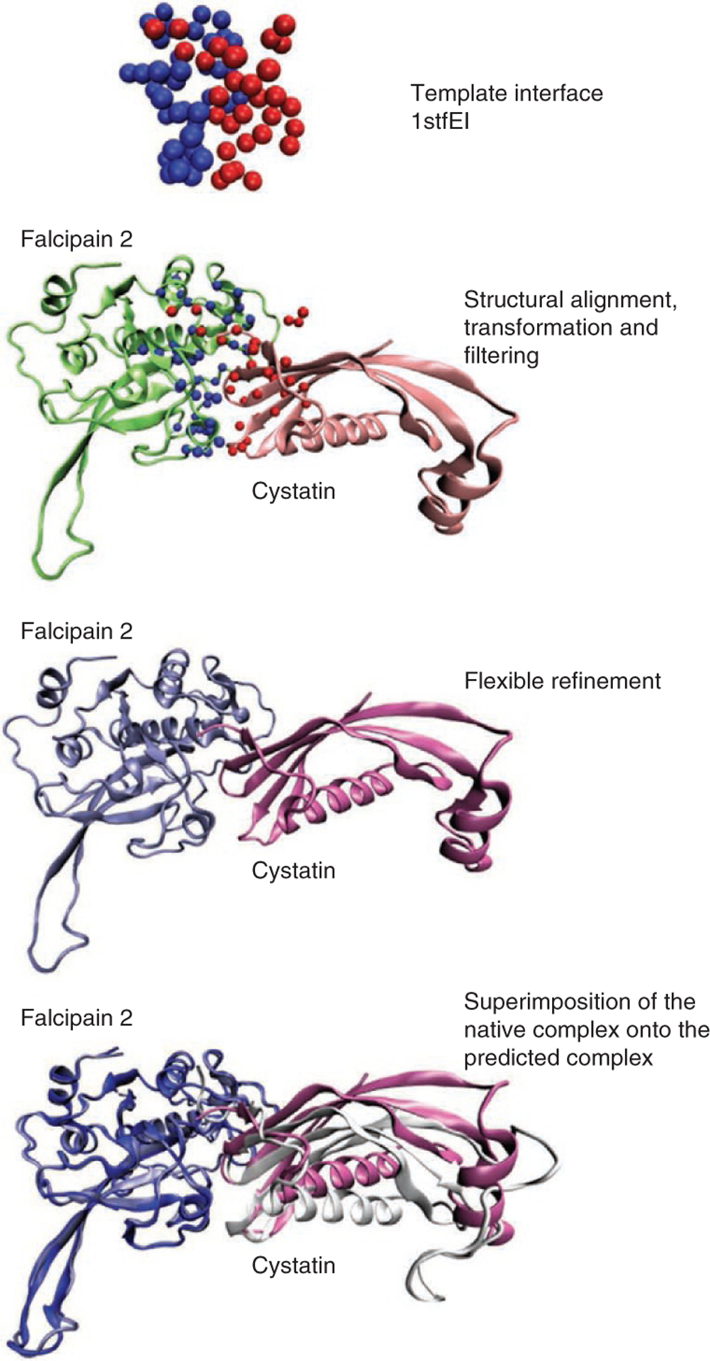
The putative Falcipain-Cystatin complex predicted by PRISM using template 1stfEI.

The matching residues between targets and template partners are available in the 1-Prediction/MULTIPROT_OUTPUT directory. To see the matching residues, change the directory to 1stfEI. From the 1stfEI_E_2ghuABCD_ 2_sol.res file, the user can find that 31 residues match between 2ghu and 1stfE at the first solution, and the RMSD between them is 0.93 Å. From the 1stfEI_I_1cew_2_sol.res file the user can observe that 17 residues match between 1cew and 1stfI at the zeroth solution and the RMSD between them is 1.58 Å.

The 1stfEI_E_2ghuABCD_log_multiprot.txt file should be checked to see which parameters are used during the structural alignment. To visualize the predicted rigid-body complex, the transformed structures onto each partner of the template interface (available in 2-DistanceCalculation/TransformedPdbs directory) should be used. Here the 1stfEI_E_2ghuABCD_1_ trans.pdb file in the 1stfEI directory indicates that this structure file is generated from the first MultiProt solution of the matching between chain E of the template interface 1stfEI and the target 2ghuABCD. Moreover, 1stfEI_I_1cew_0_ trans.pdb file in the 1stfEI directory indicates that this structure file is generated from the zeroth MultiProt solution of the matching between chain I of template interface 1stfEI and the target 1cew. In Figure 2, these transformed structures are illusturated using the VMD visualization software.

This predicted complex ranked first with a calculated global energy of − 37.34 kcal mol ^{− 1}. The second ranking solution also comes from the 1stfEI template, however, with a different MultiProt solution number.

When we compare the predicted complex to the native structure in the PDB (1yvb), we notice that the binding regions and the relative positions of the partner proteins are correctly found.

Predicted model of Chk1-p16^ink complex

As a second example, we illustrate the putative interaction between the serine/threonine protein kinase (Chk1) and cyclin-dependent kinase inhibitor p16^ink. PRISM gives two matching templates (1blxAB and 1fmaDE; see Fig. 3) for this interaction and seven interaction models. Among them, the first-ranking solution based on global energy comes from the template interface (1blxAB) between cyclin-dependent kinase 6 (Cdk6) and its inhibitor p19^ink. The sequence similarity between p16^ink and p19^ink is 38% and between Chk1 and Cdk6 is 24%. A total of 23 residues of Chk1 are matched with the left partner of 1blxAB with an RMSD of 1.49, and 42 residues of p16^ink are matched with the right partner of 1blxAB with an RMSD of 1.46. The calculated global energy for this interaction is − 29.17 kcal mol ^{− 1}.

Figure 3 |.

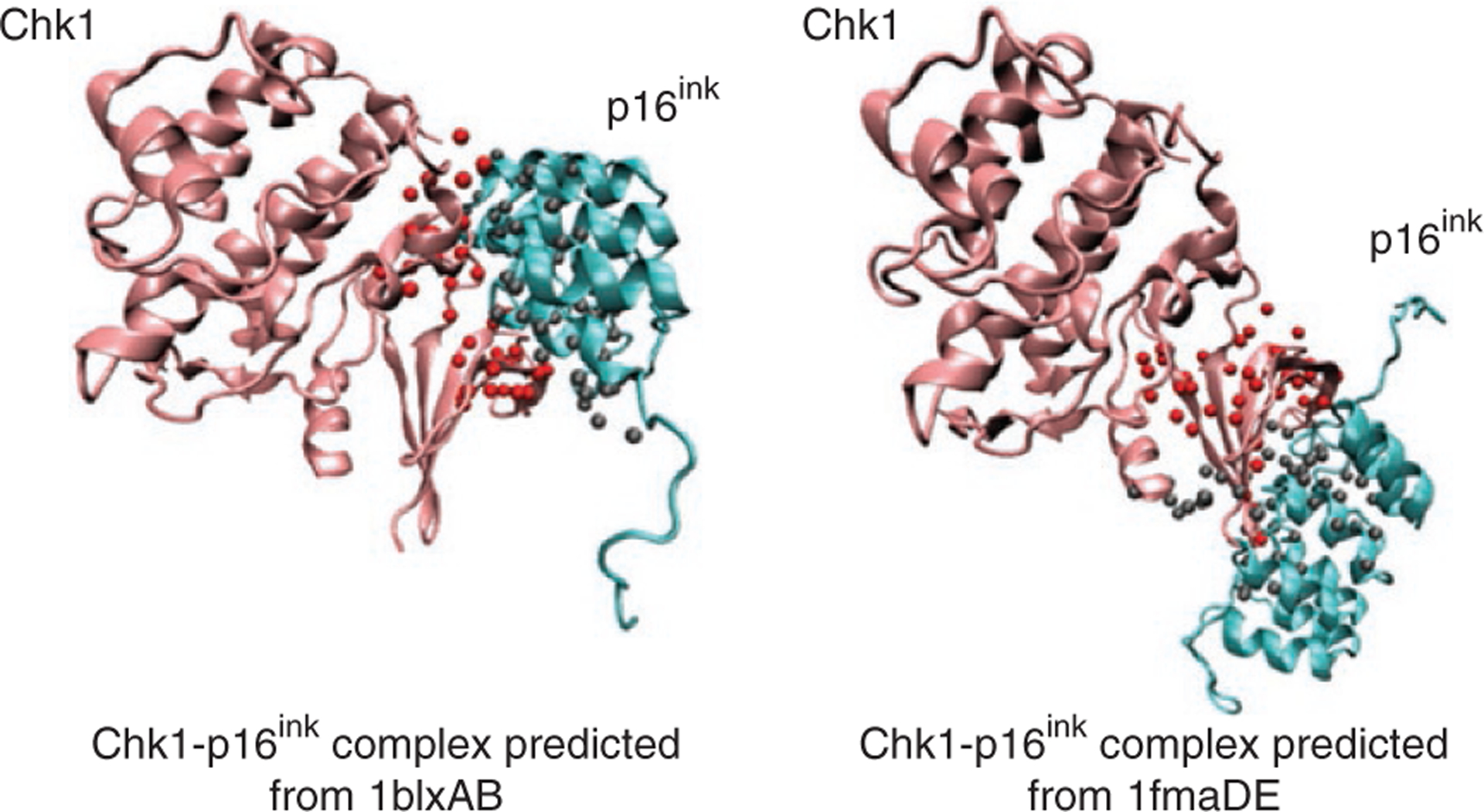
The putative Chk1-p16^ink complex predicted by PRISM using templates 1blxAB and 1fmaDE. Template interfaces are represented by balls to show the matching parts of the target surface with the template interface partners.

For ranking the solutions based on the calculated global energy, type the command line below by changing the directory to PRISM_protocol/6-FiberDock/FiberDock1.0/ENERGIES:

> sort -k 6 -n * | grep 1nvqA | grep 1a5e

The results and our previous analysis of distinct case studies show that if there is a similar template interface available in the data set, the method places the correct solution at the first place. PRISM is knowledge based; thus, if no similar interface exists in the template set, it cannot provide a model for a complex. As in any homology, or motif-based prediction method, whether global or local, the outcome is a function of the template data set.

References

- 1.Kleanthous C Protein-Protein Recognition: Frontiers in Molecular Biology (Oxford University Press, 2001). [Google Scholar]
- 2.Gavin AC et al. Functional organization of the yeast proteome by systematic analysis of protein complexes. Nature 415, 141–147 (2002). [DOI] [PubMed] [Google Scholar]
- 3.Uetz P et al. A comprehensive analysis of protein-protein interactions in Saccharomyces cerevisiae. Nature 403, 623–627 (2000). [DOI] [PubMed] [Google Scholar]
- 4.Bader GD, Betel D & Hogue CW BIND: the Biomolecular Interaction Network Database. Nucleic Acids Res. 31, 248–250 (2003). [DOI] [PMC free article] [PubMed] [Google Scholar]
- 5.Xenarios I et al. DIP, the Database of Interacting Proteins: a research tool for studying cellular networks of protein interactions. Nucleic Acids Res. 30, 303–305 (2002). [DOI] [PMC free article] [PubMed] [Google Scholar]
- 6.Berman HM et al. The protein data bank. Nucleic Acids Res. 28, 235–242 (2000). [DOI] [PMC free article] [PubMed] [Google Scholar]
- 7.Bogan AA & Thorn KS Anatomy of hot spots in protein interfaces. J. Mol. Biol 280, 1–9 (1998). [DOI] [PubMed] [Google Scholar]
- 8.Pazos F, Helmer-Citterich M, Ausiello G & Valencia A Correlated mutations contain information about protein-protein interaction. J. Mol. Biol 271, 511–523 (1997). [DOI] [PubMed] [Google Scholar]
- 9.Andrusier N, Mashiach E, Nussinov R & Wolfson HJ Principles of flexible protein-protein docking. Proteins 73, 271–289 (2008). [DOI] [PMC free article] [PubMed] [Google Scholar]
- 10.Gray JJ High-resolution protein-protein docking. Curr. Opin. Struct. Biol 16, 183–193 (2006). [DOI] [PubMed] [Google Scholar]
- 11.Halperin I, Ma B, Wolfson H & Nussinov R Principles of docking: an overview of search algorithms and a guide to scoring functions. Proteins 47, 409–443 (2002). [DOI] [PubMed] [Google Scholar]
- 12.de Vries SJ, van Dijk M & Bonvin AM The HADDOCK web server for data-driven biomolecular docking. Nat. Protoc 5, 883–897 (2010). [DOI] [PubMed] [Google Scholar]
- 13.Lesk VI & Sternberg MJ 3D-Garden: a system for modelling protein-protein complexes based on conformational refinement of ensembles generated with the marching cubes algorithm. Bioinformatics 24, 1137–1144 (2008). [DOI] [PubMed] [Google Scholar]
- 14.Cheng TM, Blundell TL & Fernandez-Recio J pyDock: electrostatics and desolvation for effective scoring of rigid-body protein-protein docking. Proteins 68, 503–515 (2007). [DOI] [PubMed] [Google Scholar]
- 15.Chen R, Li L & Weng Z ZDOCK: an initial-stage protein-docking algorithm. Proteins 52, 80–87 (2003). [DOI] [PubMed] [Google Scholar]
- 16.Schneidman-Duhovny D, Inbar Y, Nussinov R & Wolfson HJ PatchDock and SymmDock: servers for rigid and symmetric docking. Nucleic Acids Res. 33, W363–W367 (2005). [DOI] [PMC free article] [PubMed] [Google Scholar]
- 17.Caffrey DR, Somaroo S, Hughes JD, Mintseris J & Huang ES Are protein-protein interfaces more conserved in sequence than the rest of the protein surface? Protein Sci. 13, 190–202 (2004). [DOI] [PMC free article] [PubMed] [Google Scholar]
- 18.Keskin O, Tsai CJ, Wolfson H & Nussinov R A new, structurally nonredundant, diverse data set of protein-protein interfaces and its implications. Protein Sci. 13, 1043–1055 (2004). [DOI] [PMC free article] [PubMed] [Google Scholar]
- 19.Tsai CJ, Lin SL, Wolfson HJ & Nussinov R A dataset of protein-protein interfaces generated with a sequence-order-independent comparison technique. J. Mol. Biol 260, 604–620 (1996). [DOI] [PubMed] [Google Scholar]
- 20.Tsai CJ, Lin SL, Wolfson HJ & Nussinov R Protein-protein interfaces: architectures and interactions in protein-protein interfaces and in protein cores. Their similarities and differences. Crit. Rev. Biochem. Mol. Biol 31, 127–152 (1996). [DOI] [PubMed] [Google Scholar]
- 21.Keskin O & Nussinov R Similar binding sites and different partners: implications to shared proteins in cellular pathways. Structure 15, 341–354 (2007). [DOI] [PubMed] [Google Scholar]
- 22.Aytuna AS, Gursoy A & Keskin O Prediction of protein-protein interactions by combining structure and sequence conservation in protein interfaces. Bioinformatics 21, 2850–2855 (2005). [DOI] [PubMed] [Google Scholar]
- 23.Ogmen U, Keskin O, Aytuna AS, Nussinov R & Gursoy A PRISM: protein interactions by structural matching. Nucleic Acids Res. 33, W331–W336 (2005). [DOI] [PMC free article] [PubMed] [Google Scholar]
- 24.Keskin O, Nussinov R & Gursoy A PRISM: protein-protein interaction prediction by structural matching. Methods Mol. Biol 484, 505–521 (2008). [DOI] [PMC free article] [PubMed] [Google Scholar]
- 25.Kar G, Gursoy A & Keskin O Human cancer protein-protein interaction network: a structural perspective. PLoS Comput. Biol 5, e1000601 (2009). [DOI] [PMC free article] [PubMed] [Google Scholar]
- 26.Tuncbag N, Kar G, Gursoy A, Keskin O & Nussinov R Towards inferring time dimensionality in protein-protein interaction networks by integrating structures: the p53 example. Mol. Biosyst 5, 1770–1778 (2009). [DOI] [PMC free article] [PubMed] [Google Scholar]
- 27.Kar G, Keskin O, Gursoy A & Nussinov R Allostery and population shift in drug discovery. Curr. Opin. Pharmacol 10, 715–7122 (2010). [DOI] [PMC free article] [PubMed] [Google Scholar]
- 28.Acuner Ozbabacan SE, Gursoy A, Keskin O & Nussinov R Conformational ensembles, signal transduction and residue hot spots: application to drug discovery. Curr. Opin. Drug. Discov. Devel 13, 527–537 (2010). [PubMed] [Google Scholar]
- 29.Keskin O & Nussinov R Favorable scaffolds: proteins with different sequence, structure and function may associate in similar ways. Protein Eng. Des. Sel 18, 11–24 (2005). [DOI] [PubMed] [Google Scholar]
- 30.Tuncbag N, Gursoy A, Guney E, Nussinov R & Keskin O Architectures and functional coverage of protein-protein interfaces. J. Mol. Biol 381, 785–802 (2008). [DOI] [PMC free article] [PubMed] [Google Scholar]
- 31.Shatsky M, Nussinov R & Wolfson HJ A method for simultaneous alignment of multiple protein structures. Proteins 56, 143–156 (2004). [DOI] [PubMed] [Google Scholar]
- 32.Mashiach E, Nussinov R & Wolfson HJ FiberDock: flexible induced-fit backbone refinement in molecular docking. Proteins 78, 1503–1519 (2010). [DOI] [PMC free article] [PubMed] [Google Scholar]
- 33.Aloy P & Russell RB Interrogating protein interaction networks through structural biology. Proc. Natl Acad. Sci. USA 99, 5896–5901 (2002). [DOI] [PMC free article] [PubMed] [Google Scholar]
- 34.Kundrotas PJ, Lensink MF & Alexov E Homology-based modeling of 3D structures of protein-protein complexes using alignments of modified sequence profiles. Int. J. Biol. Macromol 43, 198–208 (2008). [DOI] [PubMed] [Google Scholar]
- 35.Lu L, Lu H & Skolnick J MULTIPROSPECTOR: an algorithm for the prediction of protein-protein interactions by multimeric threading. Proteins 49, 350–364 (2002). [DOI] [PubMed] [Google Scholar]
- 36.Martin J Beauty is in the eye of the beholder: proteins can recognize binding sites of homologous proteins in more than one way. PLoS Comput. Biol 6, e1000821 (2010). [DOI] [PMC free article] [PubMed] [Google Scholar]
- 37.Gunther S, May P, Hoppe A, Frommel C & Preissner R Docking without docking: ISEARCH—prediction of interactions using known interfaces. Proteins 69, 839–844 (2007). [DOI] [PubMed] [Google Scholar]
- 38.Sinha R, Kundrotas PJ & Vakser IA Docking by structural similarity at protein-protein interfaces. Proteins 78, 3235–3241 (2010). [DOI] [PMC free article] [PubMed] [Google Scholar]
- 39.Kundrotas PJ & Vakser IA Accuracy of protein-protein binding sites in high-throughput template-based modeling. PLoS Comput. Biol 6, e1000727 (2010). [DOI] [PMC free article] [PubMed] [Google Scholar]
- 40.Xie L & Bourne PE Functional coverage of the human genome by existing structures, structural genomics targets, and homology models. PLoS Comput. Biol 1, e31 (2005). [DOI] [PMC free article] [PubMed] [Google Scholar]
- 41.Xie L, Xie L & Bourne PE Structure-based systems biology for analyzing off-target binding. Curr. Opin. Struct. Biol 21, 189–199 (2011). [DOI] [PMC free article] [PubMed] [Google Scholar]
- 42.Bradford JR & Westhead DR Improved prediction of protein-protein binding sites using a support vector machines approach. Bioinformatics 21, 1487–1494 (2005). [DOI] [PubMed] [Google Scholar]
- 43.Liang S, Zhang C, Liu S & Zhou Y Protein binding site prediction using an empirical scoring function. Nucleic Acids Res. 34, 3698–3707 (2006). [DOI] [PMC free article] [PubMed] [Google Scholar]
- 44.Wells JA Systematic mutational analyses of protein-protein interfaces. Methods Enzymol. 202, 390–411 (1991). [DOI] [PubMed] [Google Scholar]
- 45.Pearson WR & Lipman DJ Improved tools for biological sequence comparison. Proc. Natl Acad. Sci. USA 85, 2444–2448 (1988). [DOI] [PMC free article] [PubMed] [Google Scholar]
- 46.Hubbard SJ & Thornton JM Naccess (Department of Biochemistry and Molecular Biology, University College, London, 1993). [Google Scholar]
- 47.Hwang H, Pierce B, Mintseris J, Janin J & Weng Z Protein-protein docking benchmark version 3.0. Proteins 73, 705–709 (2008). [DOI] [PMC free article] [PubMed] [Google Scholar]
- 48.Tuncbag N, Keskin O & Gursoy A HotPoint: hot spot prediction server for protein interfaces. Nucleic Acids Res. 38 (Suppl): W402–W406 (2010). [DOI] [PMC free article] [PubMed] [Google Scholar]
- 49.Tuncbag N, Gursoy A & Keskin O Identification of computational hot spots in protein interfaces: combining solvent accessibility and inter-residue potentials improves the accuracy. Bioinformatics 25, 1513–1520 (2009). [DOI] [PubMed] [Google Scholar]
- 50.Fischer TB et al. The binding interface database (BID): a compilation of amino acid hot spots in protein interfaces. Bioinformatics 19, 1453–1454 (2003). [DOI] [PubMed] [Google Scholar]
- 51.Thorn KS & Bogan AA ASEdb: a database of alanine mutations and their effects on the free energy of binding in protein interactions. Bioinformatics 17, 284–285 (2001). [DOI] [PubMed] [Google Scholar]
- 52.MacKerell AD et al. All-atom empirical potential for molecular modeling and dynamics studies of proteins. J. Phys. Chem. B 102, 3586–3616 (1998). [DOI] [PubMed] [Google Scholar]