

Abstract
In most US health insurance markets, plans face strong incentives to “upcode” the patient diagnoses they report to the regulator, as these affect the risk-adjusted payments plans receive. We show that enrollees in private Medicare plans generate 6% to 16% higher diagnosis-based risk scores than they would under fee-for-service Medicare, where diagnoses do not affect most provider payments. Our estimates imply that upcoding generates billions in excess public spending and significant distortions to firm and consumer behavior. We show that coding intensity increases with vertical integration, suggesting a principal-agent problem faced by insurers, who desire more intense coding from the providers with whom they contract.
Diagnosis-based subsidies have become an increasingly important regulatory tool in US health insurance markets and public insurance programs. Between 2003 and 2014, the number of consumers enrolled in a market in which an insurer’s payment is based on the consumer’s diagnosed health conditions increased from almost zero to over 50 million, including enrollees in Medicare, Medicaid, and state and federal Health Insurance Exchanges. These diagnosis-based payments to insurers are known as risk adjustment, and their introduction has been motivated by a broader shift away from public fee-for-service health insurance programs and towards regulated private markets (Gruber, 2017). By compensating insurers for enrolling high expected-cost consumers, risk adjustment weakens insurer incentives to engage in cream-skimming—that is, inefficiently distorting insurance product characteristics to attract lower-cost enrollees, as in Rothschild and Stiglitz (1976).1
The intuition underlying risk adjustment is straightforward: diagnosis-based transfer payments can break the link between the insurer’s expected costs and the insurer’s expected profitability of enrolling a chronically ill consumer. But the mechanism assumes that a regulator can objectively measure each consumer’s health state. In practice in health insurance markets, regulators infer an enrollee’s health state from the diagnoses reported by physicians during their encounters with the enrollee. This diagnosis information, usually captured in bills sent from the provider to the insurer, is aggregated into a risk score on which a regulatory transfer to the insurer is based. Higher risk scores trigger larger transfers. Insurers thus have a strong incentive to “upcode” reported diagnoses and risk scores, either via direct insurer actions or by influencing physician behavior.2 By upcoding, we mean activities that range from increased provision of diagnostic services that consumers value to outright fraud committed by the insurer or provider. The extent of such practices is of considerable policy, industry, and popular interest. Nonetheless, the few recent studies examining the distortionary effects of risk adjustment (e.g., Brown et al., 2014, Carey, 2017, Einav et al., 2015, and Geruso, Layton and Prinz, 2016) have all taken diagnosis coding as fixed for a given patient, rather than as an endogenous outcome potentially determined by physician and insurer strategic behavior. In contrast, in this paper we show that endogenous diagnosis coding is an empirically important phenomenon that has led to billions in annual overpayments by the federal government, as well as significant distortions to consumer choices.
We begin by constructing a stylized model to assess the effects of upcoding in a setting where private health plans receiving risk adjustment payments compete for enrollees against a public option. We use the model to show that when risk scores (and thus plan payments) are endogenous to the contract details chosen by the private plans, three types of distortions are introduced. First, a wedge is introduced between the efficient private contract and the private contract offered in equilibrium. Equilibrium contracts are characterized by levels of coding services (and in some cases, other healthcare services) that are too high in the sense that the marginal social cost of the service exceeds the marginal social benefit. Second, the higher intensity of coding in the private plans increases government subsidies paid to these plans, which in turn increases the cost of the program to taxpayers. Third, the higher subsidies to plans with higher coding intensity lead to equilibrium plan prices that fail to reflect the underlying social resource cost of enrolling a consumer in the plan, causing consumer choices to be inefficiently tilted toward the plans that code most intensely. An important insight from our model is that these results hold whether the differential coding intensity is caused by illegal activity such as insurer fraud or by the seemingly innocuous activity of private plans offering diagnostic services at lower out-of-pocket prices than under the public option.
We investigate the empirical importance of upcoding in the context of Medicare. For hospital and physician coverage, Medicare beneficiaries can choose between a traditional public fee-for-service (FFS) option and enrolling with a private insurer through Medicare Advantage (MA). In the FFS system, most reimbursement is independent of recorded diagnoses. Payments to private MA plans are capitated with diagnosis-based risk adjustment. As illustrated by our model, although the incentive for MA plans to code intensely is strong, doing so is not costless and a plan’s response to this incentive depends on its ability to influence the providers that assign the codes. Thus, whether and to what extent coding differs between the MA and FFS segments of the market is an empirical question.
The key challenge in identifying coding intensity differences between FFS and MA, or within the MA market segment across competing insurers, is that upcoding estimates are potentially confounded by adverse selection. An insurer might report an enrollee population with higher-thanaverage risk scores either because the consumers who choose the insurer’s plan are in worse health (selection) or because for the same individuals, the plan’s benefit design and coding practices result in higher risk scores (upcoding). We develop an approach to separately identify selection and coding differences in equilibrium. The core insight of our research design is that if the same individual would generate a different risk score under two plans and if we observe an exogenous shift in the market shares of the two plans, then we should also observe changes in the market-level average of reported risk scores. Such a pattern could not be generated or rationalized by selection, because selection can affect only the sorting of risk types across insurers or plans within the market, not the overall market-level distribution of reported risk scores.3,4
To identify coding differences, we exploit large and geographically heterogeneous increases in MA enrollment within county markets that began in 2006 following the Medicare Modernization Act. We simultaneously exploit an institutional feature of the MA program that causes risk scores to be based on prior year diagnoses. This yields sharp predictions about the timing of effects relative to changing market penetration in a difference-in-differences framework. Using the rapid withincounty changes in penetration that occurred over our short panel, we find that a 10 percentage point increase in MA penetration leads to a 0.64 percentage point increase in the reported average risk score in a county. This implies that MA plans generate risk scores for their enrollees that are on average 6.4% larger in the first year of MA enrollment than what those same enrollees would have generated under FFS. Our results also suggest that the MA coding intensity differential may ratchet up over time, reaching 8.7% by the second year of MA enrollment and continuing to grow into the third year. These are large effects. A 6.4% increase in market-level risk is equivalent to 6% of all consumers in a market becoming paraplegic, 11% developing Parkinson’s disease, or 39% becoming diabetic. While these effects would be implausibly large if they reflected rapid changes to actual population health, they are plausible when viewed as reflecting only endogenous coding behavior.
To complement our main identification strategy at the market level, we also provide individual-level evidence and a second identification strategy for a sample of Massachusetts residents. We track risk scores within consumers as they transition from an employer or individual-market commercial plan to Medicare at the age 65 eligibility threshold. We present event study difference-in-differences graphs comparing the groups that eventually choose MA and FFS. We show that during the years prior to Medicare enrollment when both groups were enrolled in similar employer and commercial plans, level differences in coding intensity were stable. Following Medicare enrollment, however, the difference in coding intensity between the MA and FFS groups spike upward, providing transparent visual evidence of a coding intensity effect of MA.
These empirical findings have specific implications for the Medicare program as well as broader implications for the regulation of private insurance markets. Medicare is the costliest public health insurance program in the world and makes up a significant fraction of US government spending. Even relative to a literature that has consistently documented phenomena leading to significant overpayments to or gaming by private Medicare plans (e.g., Ho, Hogan and Scott Morton, 2014; Decarolis, 2015; Brown et al., 2014), the size of the overpayment due to manipulable coding is striking. Absent a coding correction, our estimates imply excess payments of around $10.2 billion to Medicare Advantage plans annually, or about $650 per MA enrollee per year. The excess payments, combined with external estimates of enrollment elasticities, imply that completely removing the hidden subsidy due to upcoding would reduce the size of the MA market by 17% to 33%, relative to a counterfactual in which the Center for Medicaid and Medicare Services (CMS) made no adjustment. In 2010, toward the end of our study period, CMS began deflating MA risk payments due to concerns about upcoding, partially counteracting these overpayments.5
We view our results as addressing an important gap in the literature on adverse selection and the public finance of healthcare. Risk adjustment is the most widely implemented regulatory response to adverse selection. A few recent studies, including Curto et al. (2014) and Einav and Levin (2014), have begun to recognize the potential importance of upcoding, but the empirical evidence is underdeveloped. The most closely related prior work on coding has shown that patients’ reported diagnoses in FFS Medicare vary with the local practice style of physicians (Song et al., 2010) and that coding responds to changes in how particular codes are reimbursed by FFS Medicare for inpatient hospital stays (Dafny, 2005; Sacarny, 2014). Ours is the first study to model the welfare implications of differential coding patterns across insurers and to provide empirical evidence of the size and determinants of these differences.
Our results also provide a rare insight into the insurer-provider relationship. Because diagnosis codes ultimately originate from provider visits, insurers face a principal-agent problem in contracting with physicians. We find that coding intensity varies significantly according to the contractual relationship between the physician and the insurer. Fully vertically integrated (i.e., provider owned) plans generate 16% higher risk scores for the same patients compared to FFS, nearly triple the effect of non-integrated plans. This suggests that the cost of aligning physician incentives with insurer objectives may be significantly lower in vertically integrated firms. These results connect to a long literature concerned with the internal organization of firms (Grossman and Hart, 1986) and the application of these ideas to the healthcare industry (e.g., Gaynor, Rebitzer and Taylor, 2004 and Frakt, Pizer and Feldman, 2013). Our results also represent the first direct evidence of which we are aware that vertical integration between insurers and providers may facilitate the “gaming” of health insurance payment systems. However, these results likewise raise the possibility that strong insurer-provider contracts may also facilitate other, more socially beneficial, objectives, including quality improvements through pay-for-performance incentives targeted at the level of the insurer. This is an issue of significant policy and research interest (e.g., Fisher et al., 2012; Frakt and Mayes, 2012; Frandsen and Rebitzer, 2014), but as Gaynor, Ho and Town (2015) describe, it is an area in which there is relatively little empirical evidence.
Finally, our results connect more broadly to the economic literature on agency problems in monitoring, reporting, and auditing. Here, insurers are in charge of reporting the critical inputs that will determine their capitation payments from the regulator. The outsourcing of regulatory functions to interested parties is not unique to this setting, with examples in other parts of the healthcare system (Dafny, 2005), in environmental regulation (Duflo, Greenstone and Ryan, 2013), in financial markets (Griffin and Tang, 2011), and elsewhere. Our results point to a tradeoff in which the tools used to better align regulator and firm incentives in one way (here, risk adjustment to limit cream-skimming) may cause them to diverge in other ways (as coding intensity is increased to capture subsidies).
2. Background
We begin by outlining how a risk-adjusted payment system functions, though we refer the reader to van de Ven and Ellis (2000) and Geruso and Layton (2017) for more detailed treatments. We then briefly discuss how diagnosis codes are assigned in practice.
2.1. Risk Adjustment Background
Individuals who are eligible for Medicare can choose between the FFS public option or coverage through a private MA plan. All Medicare-eligible consumers in a county face the same menu of MA plan options at the same prices. Risk adjustment is intended to undo insurer incentives to avoid sick, high cost patients by tying subsidies to patients’ health status. By compensating the insurer for an enrollee’s expected cost on the basis of their diagnosed health conditions, risk adjustment can make all potential enrollees—regardless of health status—equally profitable to the insurer on net in expectation, even when premiums are not allowed to vary across consumer types. This removes plan incentives to distort contract features in an effort to attract lower-cost enrollees, as in Rothschild and Stiglitz (1976) and Glazer and McGuire (2000). Risk adjustment was implemented in Medicare starting in 2004 and was fully phased-in by 2007.
Formally, plans receive a risk adjustment subsidy, Si, from a regulator for each individual i they enroll. The risk adjustment subsidy supplements or replaces premiums, p, paid by the enrollee with total plan revenues given by p + Si. In Medicare Advantage, Si is calculated as the product of an individual’s risk score, ri, multiplied by some base amount, , set by the regulator: .6 In practice in our empirical setting, is set to be approximately equal to the mean cost of providing FFS in the local county market for a typical-health beneficiary, or about $10,000 per enrollee per year on average in 2014.7
The risk score is determined by multiplying a vector of risk adjusters, xi, by a vector of risk adjustment coefficients, Λ. Subsidies are therefore . Risk adjusters, xi, typically consist of a set of indicators for demographic groups (age-by-sex cells) and a set of indicators for condition categories, which are based on diagnosis codes contained in health insurance claims. In Medicare, as well as the federal Health Insurance Exchanges, these indicators are referred to as Hierarchical Condition Categories (HCCs). Below, we refer to xi as “conditions” for simplicity. The coefficients Λ capture the expected incremental impact of each condition on the insurer’s expected costs, as estimated by the regulator in a regression of total spending on the vector xi in some reference population. Coefficients Λ are normalized by the regulator so that the average risk score is equal to 1.0 in the reference population. For Medicare Advantage payment, the reference population is FFS, and risk scores for payment in year t are based on diagnoses in t − 1. The important implicit assumption underlying the functioning of risk adjustment is that conditions, xi, do not vary according to the plan in which a consumer is enrolled. In other words, diagnosed medical conditions are properties of individuals, not individual × plan matches.
2.2. Diagnosis Coding in Practice
Typically, the basis for all valid diagnosis codes is documentation from a face-to-face encounter between the provider and the patient. During an encounter like an office visit, a physician takes notes, which are passed to the billing staff in the physician’s office. Billers use the notes to generate a claim, which includes diagnosis codes, that is sent to the insurer for payment. The insurer pays claims and over time aggregates all of the diagnoses associated with an enrollee. Diagnoses are then submitted to the regulator, who generates a risk score on which payments to the insurer are based.
There are many ways for plans and providers to influence the diagnoses that are reported to the regulator. Although we reserve a more complete description of these mechanisms to Appendix Section A.2 and Figure A1, we note that insurers can structure contracts with physician groups such that the payment to the group is a function of the risk-adjusted payment that the insurer itself receives from the regulator. This directly passes through coding incentives to the physician groups. Additionally, even after claims and codes are submitted to the insurer for an encounter, the insurer or its contractor may perform a chart review—automatically or manually reviewing physician notes and patient charts to add new codes that were not originally translated to the claims submitted by the submitting physician’s office. Such additions may be known only to the insurer who edits the reports sent to the regulator, with no feedback regarding the change in diagnosis being sent to the physician or her patient. Plans may also directly or indirectly encourage more diagnostic office visits to ensure that enrollees visit the doctor and have their conditions coded. Finally, insurers may proactively contact enrollees likely to have code-able conditions and send a physician or nurse to the enrollee’s home with the sole purpose of coding the relevant, reimbursable diagnoses for the current plan year. As we discuss in Section 8, this issue is of particular concern to the Medicare regulator, CMS, as these visits, often performed by third-party contractors, appear to often be unmoored from any follow-up care or even communication with the patient’s normal physician.
None of the insurer activities targeted at diagnosis coding take place in FFS because providers under the traditional system are paid directly by the government, and the basis of these payments outside of hospital settings is procedures, not diagnoses. This difference in incentive structure between FFS and MA makes Medicare a natural setting for studying the empirical importance of differential coding intensity.
3. Model of Risk Adjustment with Endogenous Coding
In this section, we present a stylized model of firm behavior in a competitive insurance market where payments are risk adjusted. The model illustrates how distortions to public spending, consumers’ plan choices, and insurers’ benefit design can arise if risk scores are endogenous to a plan’s behavior.
3.1. Setup
We consider an insurance market similar to Medicare, where consumers choose between a public option plan (FFS) and a uniform private plan alternative offered by insurers in a competitive market (MA). An MA plan consists of two types of services and a price: {δ, γ; p}. Coding services, δ, include activities like insurer chart review. These services affect the probability that diagnoses are reported. We also allow them to impact patient utility. All other plan details are rolled up into a composite healthcare service, γ. We allow that any healthcare service or plan feature may impact reported diagnoses. For example, zero-copay specialist visits may induce some consumer moral hazard and alter the probability that a consumer visits a specialist and thus influence the probability that a marginal (correct) diagnosis is recorded.8 Services δ and γ are measured in the dollars of cost they impose on the MA plan.
Denote the consumer valuations of δ and γ in dollar-metric utility as v(δ) and w(γ), respectively. We assume utility is additively separable in v and w with vʹ > 0, wʹ > 0, vʺ < 0, and wʺ < 0. The FFS option offers reservation utility of for the mean consumer. Its price is zero. A taste parameter, σi, which is uncorrelated with costs net-of-risk adjustment, distinguishes consumers with idiosyncratic preferences over the MA/FFS choice. The purpose of the assumption of orthogonality between the taste parameter and costs is to simplify the exposition of the consequences of upcoding. The conclusions we draw from this stylized model do not rely on this assumption.9 Utility of the MA plan is thus v(δ)+w(γ)+σi. Using ζi to capture mean zero ex ante health risk that differs across consumers, expected costs in MA are ci, MA = δ + γ + ζi.
To narrow focus here on the distortions generated by upcoding even when risk adjustment succeeds in perfectly in counteracting selection, we make two simplifying assumptions. First, we assume that consistent with the regulatory intent of risk adjustment, there is no uncompensated selection after risk adjustment payments are made: Risk adjustment payments net out idiosyncratic health risk in expectation, allowing us to ignore the mean zero ζi term when considering firm incentives. Expected (net) marginal costs are equal to expected (net) average costs and are δ + γ. To simplify exposition, we assume further that there is no sorting by health status across plans in equilibrium. This implies that the mean risk score within the MA plan is 1.10
MA plans charge a premium p and receive a per-enrollee subsidy, Si, that is a function of the risk score, ri, MA, the plan reports. Following the institutional features of Medicare, , where is a base payment equal to the cost of providing FFS to the typical health Medicare beneficiary in the local market. Defining ρi(δ, γ) ≡ ri, MA − ri, FFS as the difference between the risk score each beneficiary would have generated in MA relative to the risk score she would have generated in FFS, the average (per capita plan-level) MA subsidy is then . This simplifies to if we assume, counter to the empirical facts we document, that risk scores are fixed properties of individuals and invariant to MA enrollment.
3.2. Planner’s Problem
To illustrate how the competitive equilibrium may yield inefficiencies, consider as a benchmark a social planner who is designing an MA alternative to FFS, and whose policy instruments include δ, γ, and the supplemental MA premium p. The planner takes as given the cost, zero price, and reservation utility of the FFS option, though we return to the issue of the social cost of FFS further below.11 The planner maximizes consumer utility generated by MA plan services, net of the resource cost of providing them:
| (1) |
First order conditions with respect to γ and δ yield v’(δ∗) = 1 and w’(γ∗) = 1. At the optimal provision of healthcare services and the optimal investment in coding, the marginal consumer utility of γ and δ equal their marginal costs, which is 1 by construction.
Next consider the price p∗ that efficiently allocates consumers to the FFS and MA market segments. In an efficient allocation, consumers choose the MA plan if and only if the social surplus generated by MA for them exceeds the social surplus generated by FFS.12 This condition is
| (2) |
A consumer chooses MA only if her valuation of MA minus the premium exceeds her reservation utility in the FFS option at its zero price: . This criterion for a consumer choosing MA matches the efficient allocation condition in (2) if . Therefore, the planner sets the MA/FFS price difference equal to the difference between resources consumed under MA (δ+γ) versus under FFS . This is the familiar result that (incremental) prices set equal to (incremental) marginal costs induce efficient allocations.
3.3. Insurer Incentives and Coding in Equilibrium
We next consider an MA insurer who sets {δ, γ; p} in a competitive equilibrium. Because consumer preferences are identical up to a taste-for-MA component that is uncorrelated with δ and γ and is uncorrelated with costs net of risk adjustment, there is a single MA plan identically offered by all insurers in equilibrium. Insurers will offer the contract that maximizes consumer surplus subject to the zero-profit condition, or else face zero enrollment. The zero profit condition here is p+S = δ+γ. As described above, subsidies are a function of the level of healthcare and coding services chosen by the plan: . The insurer’s problem, which simplifies to maximizing consumer surplus, is then
| (3) |
where we have substituted marginal costs net of the subsidy for the price using the zero profit condition. The first-order conditions yield and . If risk scores were exogenous to δ and γ and fixed at their FFS level, then and S would amount to a lump sum subsidy. In this case service provision would be set to the socially optimal level in a competitive equilibrium, with and . Additionally, the competitive equilibrium MA premium would equal the premium that efficiently sorts consumers between MA and FFS: . Efficient plan design and pricing would be achieved.
Generally, however, when the subsidy is endogenous to γ and δ, inefficiencies will arise. Given diminishing marginal utility of δ and γ, and assuming that more coding services and more healthcare services lead to higher risk scores, competition under endogenous risk scores induces MA insurers to set the levels of both healthcare spending and coding inefficiently high: and . This is because on the margin, insurers are rewarded via the subsidy for setting service provision above the level implied by the tradeoff between satisfying consumer preferences and incurring plan costs. The intuition here is the standard public finance result that taxes or subsidies that are responsive to an agent’s behaviors induce inefficient behaviors relative to the first best. We show in Appendix Section A.4 that identical distortions arise in the incentives for setting δ and γ in an imperfectly competitive market with endogenous coding. Given the first order conditions above, the competitive equilibrium premium will be equal to because the zero profit condition forces the additional subsidy to be passed through to the consumer as a lower premium. This price below marginal cost induces inefficient sorting, tilting consumer choices towards MA.
3.4. Welfare
Although we do not estimate the welfare impacts of upcoding in this paper, modeling welfare is instructive for understanding the implications of the coding differences we identify. To build up a welfare expression, let θMA and θFFS denote the fraction of the Medicare market enrolled in the MA and FFS segments, respectively, with . Here, θFFS expresses the fraction of the population for whom idiosyncratic preferences for MA, σ ∼ F(·), are less than the mean difference in consumer surplus generated by FFS at its zero price relative to the MA alternative at its price p(δ, γ). MA’s market share is simply 1 − θFFS. Let ΦMA and ΦFFS tally the per-enrollee social surplus generated by each option, excepting the idiosyncratic taste component, σ.13
Welfare is the social surplus generated for enrollees in each of the MA and FFS market segments minus the distortionary cost of raising public funds to subsidize (both segments of) the market. Using tildes to indicate the competitive equilibrium outcomes with endogenous risk scores, equilibrium social surplus per capita is
| (4) |
where the integral term accounts for the variable component of surplus generated by idiosyncratic tastes for MA among those who enroll in MA. The last term captures the distortionary cost of financing Medicare. It is the government’s expenditure on FFS plus its expenditure on MA, multiplied by the excess burden of raising public funds, κ. Taking per capita FFS costs, , as given and assuming that the levels of δ and γ chosen by the MA plans generate risk scores that exceed the FFS risk scores, public spending on the Medicare program increases for every consumer choosing MA instead of FFS. Without differential coding, FFS and MA risk scores are the same (ρ = 0) and the public funds term would reduce to , which is not a function of the share of beneficiaries choosing MA.
Next consider the welfare loss associated with endogenous coding by comparing the social surplus in (4) to a (possibly infeasible) regime in which risk scores are exogenously determined and service levels are optimally set. With defined as above, let WExo denote the social surplus per capita in a competitive equilibrium in which risk scores are exogenous to plan choices, which we show above replicates the social planner’s solution in the same setting. Using stars to indicate plan features (δ∗, γ∗) and market outcomes (θ∗, Φ∗) in the case of first best service levels and exogenously determined subsidies that do not depend on those levels, this difference is
| (5) |
The expression, derived in Appendix A.5, reveals three sources of inefficiency that arise from linking the MA subsidy to risk scores that plans can influence: (i) a subsidy “overpayment” to MA plans that is not balanced by a reduction in FFS spending, thus expanding overall spending on the Medicare program and the consequent public funds cost; (ii) an allocative inefficiency in which consumers sort to the wrong FFS vs MA market segment because the MA prices are distorted; and (iii) a resource use inefficiency in which plans over-invest in services that affect risk scores relative to the value of these plan features to consumers.
Although we are not able to estimate the necessary parameters for assessing the extent of each of the three inefficiencies, our estimation recovers , the differential coding intensity in MA relative to FFS, which is an input to term (i). Because the base payment and the fraction of the market in MA are quantities that are directly observable, we can calculate term (i) after recovering . We do this in Section 8.1. Note that estimating term (i) does not require us to pin down the mechanism behind the MA/FFS coding difference. It requires only generating an unbiased estimate of the difference itself. Note also that this quantity reflects the difference between actual MA coding and FFS coding, not the difference between actual MA coding and optimal MA coding, ρ(δ∗, γ∗), which too could differ from FFS coding.14
Term (ii) is a function of how many consumers choose MA in equilibrium relative to the first best: . In Section 8.2 we combine our estimates of ρ with parameters from the MA literature to calculate how different the size of the MA market would be relative to what we observe if the differential MA subsidy to coding were removed. This sheds some light on the size of the distortion in (ii).
Term (iii) reveals that even if consumers place positive value on the marginal coding services provided by plans (i.e., ), there is a welfare loss with endogenous risk scores because the incremental valuation of the coding services is less than the incremental social cost . Insurers don’t internalize the full social cost of these services because the subsidy partially compensates them for coding-related activities at a rate .
Because our empirical strategy is not designed to recover consumer preferences over healthcare services, we cannot estimate term (iii). The term nonetheless provides useful intuitions in interpreting our results. For example, it implies that inefficiencies may also arise in the provision of non-coding services such as annual wellness visits and lab tests if these have incidental impacts on the probability that a diagnosis is captured. In the controversial case of MA home health risk assessments, even if home visits provide value to enrollees, such valuations are likely to fall below the social cost of provision and would not have been included in plans if insurers were responding only to consumer preferences over healthcare services. Likewise, it is possible in principle that consumers get value out of intensive coding, perhaps because physicians have more information about their conditions and can thus provide better treatment. The model shows that while improved coding may be valued by consumers, profit maximization implies that in equilibrium its value will be exceeded by its (social resource) cost, so the additional coding is inefficient.
Equation (5) also informs how the government, as an actor, may or may not address the specific inefficiencies caused by the coding incentive. The primary strategy currently used by regulators to address the implicit MA overpayment is to deflate private plan risk scores by some factor before determining payments. If risk scores were reduced by an amount η set equal to ρ, then the additional cost of public funds (term i), could be eliminated. However, this would not eliminate welfare losses due to inefficient sorting (term ii), as the new net-of-subsidy MA price still would not accurately reflect the differential cost of FFS vs. MA. Risk score deflation also would not eliminate surplus losses due to inefficient contracts (term iii) because the insurer’s marginal incentives to code intensely would not be changed by subtracting a fixed term from the subsidy.15,16
Finally, we note that the welfare analysis here is relative to a first best in a setting with exogenously determined subsidies. It assumes away other distortions in the MA market that affect prices and the design of plan services. Although our focus is on the specific distortions generated by the coding incentive, these are just one piece in the broader landscape of efficiency and welfare in the MA program, and a complete second best analysis must account for other simultaneous market failures.
3.5. Upcoding, Complete Coding, and Socially Efficient Coding
Motivated by the model, we define upcoding in MA as the difference between the risk score a consumer would receive if she enrolled in an MA plan and the score she would have received had she enrolled in FFS: ρi(δ, γ) ≡ ri, MA − ri, FFS. It is simply the differential coding intensity between FFS and MA, which maps to the first source of inefficiency documented in Equation (5). It is the parameter required to measure the excess spending (and, therefore the excess burden) associated with a consumer choosing MA in place of FFS.
As an alternative benchmark, one could define upcoding as many physicians do: the difference between a reported risk score and the risk score that would be assigned to an individual if coding were “complete” in the sense that the individual was objectively examined and all conditions were recorded. Even setting aside the practical and conceptual difficulties with such a definition,17 our model highlights that such a benchmark of “complete” coding ignores the social resource costs of the coding, a key component of social welfare. This highlights an important distinction between the economist’s and physician’s view of this phenomenon.
4. Identifying Upcoding in Selection Markets
The central difficulty of empirically identifying upcoding arises from selection on risk scores. At the health plan level, average risk scores can differ across plans competing in the same market either because coding differs for identical patients, or because patients with systematically different health conditions select into different plans. Our solution to the identification problem is to focus on market level averages of risk scores, rather than plan risk scores. Whereas the reported risk composition of plans can reflect both coding differences and selection, risk scores calculated at the market level will not be influenced by selection—that is, by how consumers sort themselves across plans within the market. We show in this section that changes in risk scores at the market level that result from consumers shifting between plans within the market identify differences in coding.
To see this, consider how the mean risk score in a county changes as local Medicare beneficiaries shift from FFS to MA. Define the risk score an individual would have received in FFS as . Define the same person’s risk score had they enrolled in MA as , where is the mean coding intensity difference between MA and FFS across all i and where we allow for individual-level heterogeneity in the difference between MA and FFS risk scores as captured by ei. Using as the indicator function for choosing MA, an individual’s realized risk score is then . Let ϵ(θ) be the average value of ei for the set of consumers on the MA/FFS margin when the MA enrollment share equals θ. The county-level mean risk score as a function of MA enrollment can thus be written as , where expresses the unconditional expectation of . The integral measures the mean MA/FFS coding difference among the types choosing MA. In the simple case of no individual heterogeneity in the size of the coding effect, and the derivative of the county-level risk score with respect to changes in MA share exactly pins down the difference in coding intensity. That is, . In the more complex case in which there is arbitrary heterogeneity in ϵi, the slope identifies not the mean differential coding intensity across all i, which is , but rather the coding difference for the marginal consumers generating the change in market share. (See Appendix A.7.)
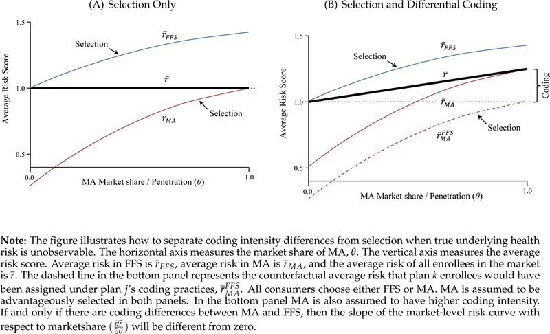
Figure 1 provides a graphical intuition of this idea for the simple case of a constant additive effect of MA enrollment on risk scores. We depict two market segments that are intended to align with FFS and MA, though the intuitions apply to considering coding differences across MA plans within the MA market segment as well. In the figure, all consumers choose either FFS or MA. The market share of MA increases along the horizontal axis. The MA segment is assumed to be advantageously selected on risk scores, so that the risk score of the marginal enrollee is higher than that of the average enrollee. Thus, the average risk within the MA segment is lower at lower levels of θMA.18
Figure 1:
Identifying Coding Differences in Selection Markets
In the top panel of Figure 1, we plot the baseline case of no coding differences across plans . The top panel shows three curves: the average risk in FFS , the average risk in MA , and the average risk of all enrollees in the market . As long as there is no coding difference between the plans or market segments, the market-level risk , which is averaged over all enrollees, is constant as θ changes. This is because reshuffling enrollees across plan options within a market does not affect the market-level distribution of underlying health conditions. Nor does it affect risk scores if the mapping from health to recorded diagnoses does not vary with plan choice (which is by assumption here). In the bottom panel of Figure 1 we add differential coding. For reference, the dashed line in the figure represents the counterfactual average risk that MA enrollees would have been assigned under FFS coding intensity, . The key difference in the bottom panel is that if MA/FFS coding intensity differs, then market-level risk changes as a function of MA’s market share. This is because even if the population distribution of actual health conditions is fixed, market-level reported risk scores would change as market shares shift between plans with higher and lower coding intensity. As the marginal consumer switches from FFS to MA, she increases θMA by a small amount and simultaneously increases the average reported risk in the market by a small amount (by moving to a plan that assigns her a higher score). Thus the slope identifies . We estimate this slope in the empirical exercise that follows.
We show in Appendix A.7 that the core intuition of Figure 1 holds if we relax many of our assumptions, including additive baseline risk and the direction and monotonicity of selection. Additionally, we show that when heterogeneity in risk is correlated with θ, estimates of are “local,” identifying the average coding difference across the set of consumers who are marginal to the variation in MA penetration used in estimation, analogous to the treatment on the treated. As explained in Appendix A.7, this local estimate is, conveniently, likely to be the parameter of interest for determining excess public spending.
5. Setting and Empirical Framework
5.1. Data
Estimating the slope requires observing market-level risk scores as MA penetration changes. We obtained yearly county-level averages of risk scores and MA enrollment by plan type from CMS for 2006 through 2011.19 MA enrollment is defined as enrollment in any MA plan type, including managed care plans like Health Maintenance Organizations (HMOs) and Preferred Provider Organizations (PPOs), private fee-for-service (PFFS) plans, and employer MA plans. In our main specifications, we consider the Medicare market as divided between the MA and FFS segments and collapse all MA plan types together. We later estimate heterogeneity in coding within MA, across its various plan type components. MA penetration (θMA) is the fraction of all beneficiary-months of a county-year spent in an MA plan. Average risk scores are weighted by the fraction of the year each beneficiary was enrolled in Medicare.
All analysis of risk scores in the national sample is conducted at the level of market averages, as the regulator does not generally release individual-specific risk adjustment data for MA plans. We supplement these county-level aggregates with administrative data on demographics for the universe of Medicare enrollees from the Medicare Master Beneficiary Summary File (MBSF) for 20062011. These data allow us to construct county-level averages of the demographic (age and gender) component of risk scores, which we use in a falsification test.
Table 1 displays summary statistics for the balanced panel of 3,128 counties that make up our analysis sample. The columns compare statistics from the introduction of risk adjustment in 2006 through the last year for which data are available, 2011. These statistics are representative of counties, not individuals, since our unit of analysis is the county-year. The table shows that risk scores, which have an overall market mean of approximately 1.0, are lower within MA than within FFS, implying that MA selects healthier enrollees.20 Table 1 also shows the dramatic increase in MA penetration over our sample period, which comprises one part of our identifying variation.
Table 1:
Summary Statistics
| Analysis Sample: Balanced Panel of Counties, 2006 to 2011 | |||||
|---|---|---|---|---|---|
| 2006 | 2011 | ||||
| Mean | Std. Dev | Mean | Std. Dev | Obs | |
| MA penetration (all plan types) | 7.1% | 9.1% | 16.2% | 12.0% | 3128 |
| Risk (HMO/PPO) plans | 3.5% | 7.3% | 10.5% | 10.5% | 3128 |
| PFFS plans | 2.7% | 3.2% | 2.7% | 3.7% | 3128 |
| Employer MA plans | 0.7% | 2.2% | 2.8% | 4.3% | 3128 |
| Other MA plans | 0.2% | 1.4% | 0.0% | 0.0% | 3128 |
| MA-Part D penetration | 5.3% | 8.0% | 13.1% | 10.8% | 3128 |
| MA non-Part D penetration | 1.8% | 3.0% | 3.0% | 4.0% | 3128 |
| Market risk score | 1.000 | 0.079 | 1.000 | 0.085 | 3128 |
| Risk score in TM | 1.007 | 0.082 | 1.003 | 0.084 | 3128 |
| Risk score in MA | 0.898 | 0.171 | 0.980 | 0.147 | 3124 |
Note: The table reports county-level summary statistics for the first and last year of the main analysis sample. The sample consists of 3,128 counties for which we have a balanced panel of data on Medicare Advantage penetration and risk scores. MA penetration in the first row is equal to the beneficiary-months spent in Medicare Advantage divided by the total number of Medicare months in the county × year. The market risk score is averaged over all Medicare beneficiaries in the county and normed to 1.00 nationally in each year.
5.2. Identifying Variation
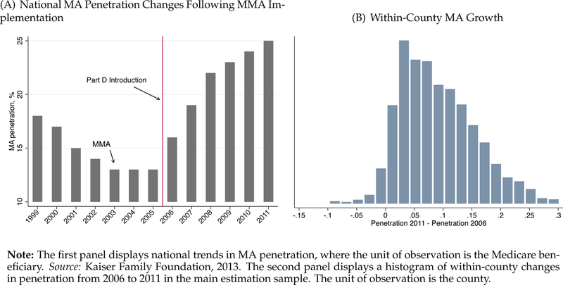
We exploit the large and geographically heterogeneous increases in MA penetration that followed implementation of the Medicare Modernization Act of 2003. The Act introduced Medicare Part D, which was implemented in 2006 and added a valuable new prescription drug benefit to Medicare. Because Part D was available solely through private insurers and because insurers could combine Part D drug benefits and MA insurance under a single contract, this drug benefit was highly complementary to enrollment in MA. Additionally, MA plans were able to “buy-down” the Part D premium paid by all Part D enrollees. This, along with increases in MA benchmark payments in some counties, led to fast growth in the MA market segment (Gold, 2009). In Panel A of Figure 2, we put this timing in historical context. Following a period of decline, MA penetration doubled nationally between 2005 and 2011. Panel B of the figure shows that within-county penetration changes were almost always positive, though the size of these changes varied widely. A map of changes by county, presented in Figure A3, shows that this MA penetration growth was not limited to certain regions or to urban or rural areas.
Figure 2:
Identification: Within-County Growth in Medicare Advantage Penetration
Our main identification strategy relies on year-to-year variation in penetration within geographic markets to trace the slope of the market average risk curve, . The identifying assumption in our difference-in-differences framework is that year-to-year growth in MA enrollment within counties did not track year-to-year variation in the county’s actual population-level health. The assumption is plausible because the incidence of the types of chronic conditions used in risk scoring (such as diabetes and cancer) is unlikely to change sharply year-to-year. In contrast, reported risk can change sharply due to coding differences as the local Medicare population shifts to MA. In support of the identifying assumption, we show that there is no correlation between within-county changes in θMA and within-county changes in a variety of demographic, morbidity, and mortality outcomes that could in principle signal health-motivated demand shifts.
We also exploit an institutional feature of how risk scores are calculated in MA to more narrowly isolate the identifying variation. Under Medicare rules, the risk scores that are assigned to beneficiaries and used as a basis for payment in calendar year t are based on diagnoses derived from service provision in calendar year t − 1. This implies, for example, that if an individual moves to MA from FFS during open enrollment in January of a given year, the risk score for her entire first year in MA will be based on diagnoses she received while in FFS during the prior calendar year. Only after the first year of MA enrollment will the risk score of the switcher include diagnoses she received while enrolled with her MA plan. Changes in risk scores due to upcoding should therefore not occur in the same year as the identifying shift in enrollment. We test this.
5.3. Econometric Framework
We estimate difference-in-differences models of the form:
| (6) |
where is the average market-level risk in county c of state s in year t, and θMA denotes MA penetration, which ranges from zero to one. County and year fixed effects are captured by γc and γt, so that effects β are identified within counties over time. County fixed effects control for any unobserved constant local factors that could simultaneously affect population health and MA enrollment, such as medical infrastructure, consumer health behaviors, or physician practice styles (Song et al., 2010; Finkelstein, Gentzkow and Williams, 2016). Year fixed effects are included to capture any changes in the composition of Medicare at the national level. Xsct is a vector of time-varying county characteristics described in more detail below. The subscript τ in the summation indicates the timing of the penetration variable, θ, relative to the timing of the reported risk score. This specification allows flexibility in identifying the timing of effects. Coefficients βτ multiply contemporaneous MA penetration (τ = t), leads of MA penetration (τ > t), and lags of MA penetration (τ < t). Contemporaneous and leading βs serve as placebo tests, revealing whether counties were differentially trending in the dependent variable prior to when risk scores could have plausibly been affected by upcoding.
The coefficient of interest is βt−1 because of the institutional feature described above in which risk scores are calculated based on the prior full year’s medical history, so that upcoding could plausibly affect risk scores only after the first year of MA enrollment. A positive coefficient on lagged penetration indicates more intensive coding in MA relative to FFS.
6. Results
6.1. Main Results
Table 2 reports our main results. The coefficient of interest is on lagged MA penetration. In column 1, we present estimates of the baseline model controlling for only county and year fixed effects. The difference-in-differences coefficient indicates that the market-level average risk score in a county increases by about 0.07—approximately one standard deviation—as lagged MA penetration increases from 0% to 100%. Because risk scores are scaled to have a mean of one, this implies that an individual’s risk score in MA is about 7% higher than it would have been under fee-for-service (FFS) Medicare. In column 2, we add linear state time trends, and in column 3, we add time-varying controls for county demographics.21 Across specifications, the coefficient on lagged MA penetration is stable.22
Table 2:
Main Results: Impacts of MA Expansion on Market-Level Reported Risk
| Dependent Variable: County-Level Average Risk Score |
||||
|---|---|---|---|---|
| (1) | (2) | (3) | (4) | |
| MA Penetration t (placebo) | 0.007 (0.015) |
0.001 (0.019) |
0.001 (0.019) |
0.006 (0.017) |
| MA Penetration t-1 | 0.069** (0.011) |
0.067** (0.012) |
0.064** (0.011) |
0.041** (0.015) |
| MA Penetration t-2 | 0.046* (0.022) |
|||
| Main Effects | ||||
| County FE | X | X | X | X |
| Year FE | X | X | X | X |
| Additional Controls | ||||
| State X Year Trend | X | X | X | |
| County X Year Demographics | X | X | ||
| Mean of Dep. Var. | 1.00 | 1.00 | 1.00 | 1.00 |
| Observations | 15,640 | 15,640 | 15,640 | 12,512 |
Note: The table reports coefficients from difference-in-differences regressions in which the dependent variable is the average risk score in the market (county). Effects of contemporaneous (t) and lagged (t − 1, t − 2) Medicare Advantage (MA) penetration are displayed. Because MA risk scores are calculated using diagnosis data from the prior plan year, changes in MA enrollment can plausibly affect reported risk scores via differential coding only with a lag. Thus, contemporaneous penetration acts as a placebo test. Observations are county × years. The inclusion of an additional lag in column 4 reduces the available panel years and the sample size. All specifications include county and year fixed effects. Column 2 additionally controls for state indicators interacted with a linear time trend. Columns 3 and 4 additionally control for the demographic makeup of the county × year by including 18 indicator variables capturing the fraction of the population in 5-year age bins from 0 to 85 and >85. Standard errors in parentheses are clustered at the county level.
p < 0.05
p < 0.01.
An alternative interpretation of these results is that, contrary to our identifying assumption, the estimates reflect changes in underlying health in the local market. Although we cannot rule out this possibility entirely, the coefficient estimates for the contemporaneous MA penetration variable, reported in the first row of Table 2, constitute a kind of placebo test. If there were a contemporaneous correlation between MA penetration changes and changes in risk scores, it would suggest that the health of the population was drifting in a way that was spuriously correlated with the identifying variation. Contrary to this, the placebo coefficients are very close to zero and insignificant across all specifications. Effects appear only with a lag, consistent with the institutions described above.23
As discussed above, switchers from FFS to MA carry forward their old FFS risk scores for their first MA plan year. For newly-eligible consumers aging into Medicare at 65 and choosing MA, the timing is more complex. Diagnosis-based risk scores may not be assigned until after two calendar years with MA enrollment due to the details of how new enrollees are treated by the risk adjustment system.24 To investigate, in column 4 of Table 2 we include a second lag of θ in the regression. Each coefficient represents an independent effect, so that point estimates in column 4 indicate a cumulative upcoding effect of 8.7% (=4.1+4.6) after two years. The timing is consistent with some of the changes in θ being driven by newly-eligible beneficiaries. It is also consistent with the possibility that even among switchers, for whom effects could begin to be seen after one year of enrollment, coding intensity differentials ratchet up over the time a beneficiary stays with an MA plan (Kronick and Welch, 2014). This is plausible, as some insurer strategies for increasing coding intensity, such as prepopulating physician notes with past years’ diagnoses, require a history of contact with the patient.
To put the size of our main estimate in context, a 6.4% increase in market-level risk (Table 2, column 3) would be associated with 6% of all consumers in a market becoming paraplegic, 11% developing Parkinson’s disease, or 39% becoming diabetic. The effects we estimate would be implausibly large if they reflected true (high frequency) changes in underlying population health, rather than coding activity.
6.2. Falsification Tests
As further support of the identifying assumption, in Table 3 we conduct a series of falsification tests intended to uncover any correlation between changes in MA penetration and changes in other timevarying county characteristics not plausibly affected by upcoding. Each column in the table replicates specifications from Table 2, but with alternative dependent variables. In columns 1 and 2, the dependent variable is the demographic portion of the risk score. The demographic portion of the risk score is based only on age and gender, with this information retrieved from the Social Security Administration rather than reported by the plan. Both the lagged and contemporaneous coefficients are near zero and insignificant, showing no correlation between MA penetration and the portion of the risk score that is exogenous to insurer and provider actions.25
Table 3:
Falsification Tests: Effects on Measures Not Manipulable by Coding
| Ependent Variable, Calculated as County Average: |
||||||
|---|---|---|---|---|---|---|
| Demographic Portion of Risk Score |
Mortality Over 65 |
Cancer Incidence Over 65 |
||||
| (1) | (2) | (3) | (4) | (5) | (6) | |
| MA Penetration t | 0.001 (0.002) |
0.001 (0.002) |
0.002 (0.002) |
0.002 (0.003) |
−0.005 (0.005) |
−0.005 (0.005) |
| MA Penetration t-1 | 0.000 (0.002) |
−0.001 (0.002) |
−0.002 (0.002) |
−0.002 (0.002) |
0.001 (0.004) |
0.003 (0.005) |
| Main Effects | ||||||
| County FE | X | X | X | X | X | X |
| Year FE | X | X | X | X | X | X |
| Additional Controls | ||||||
| State X Year Trend | X | X | X | X | X | X |
| County X Year Demographics | X | X | X | |||
| Mean of Dep. Var. | 0.485 | 0.485 | 0.048 | 0.048 | 0.023 | 0.023 |
| Observations | 15,640 | 15,640 | 15,408 | 15,408 | 3,050 | 3,050 |
Note: The table reports estimates from several falsification exercises in which the dependent variables are not in principle manipulable by coding activity. The coefficients are from difference-in-differences regressions of the same forms as those displayed in Table 2, but in which the dependent variables are changed, as indicated in the column headers. In columns 1 and 2, the dependent variable is the average demographic risk score in the county-year, calculated by the authors using data from the Medicare Beneficiary Summary File based on age, gender, and Medicaid status, but not diagnoses. In columns 3 and 4, the dependent variable is the mortality rate which is derived using data from the National Center for Health Statistics. In columns 5 and 6, the dependent variable is the cancer incidence rate from the Surveillance, Epidemiology, and End Results (SEER) Program of the National Cancer Institute, which tracks cancer rates independently from rates observed in claims data. The smaller sample size in columns 3 and 4 is due to the NCHS suppression of small cells. The smaller sample size in columns 5 and 6 reflects the incomplete geographical coverage of SEER cancer incidence data. Cancer incidence and mortality are both calculated conditional on age ≥ 65. Observations are county × years. Controls are as described in Table 2. Standard errors in parentheses are clustered at the county level.
p < 0.05
p < 0.01.
In columns 3 through 6 of Table 3, we test whether changes in MA penetration are correlated with independent (non-insurer reported) measures of mortality and morbidity. Mortality is independently reported by vital statistics. For morbidity, finding data that is not potentially contaminated by the insurers’ coding behavior is challenging. The typical sources of morbidity data are the medical claims reported by insurers. Here we rely on cancer incidence data from the Surveillance, Epidemiology, and End Results (SEER) Program of the National Cancer Institute, which operates an independent data collection enterprise to determine diagnoses. Cancer data is limited to the subset of counties monitored by SEER, which accounted for 27% of the US population in 2011 and 25% of the population over 65. In columns 3 and 4, the dependent variable is the county × year mortality rate among residents age 65 and older. In columns 5 and 6, it is the SEER-reported cancer incidence in the county × year among residents age 65 and older. Across all of the outcomes in Table 3, coefficients on contemporaneous and lagged MA penetration are consistently close to zero. In Table A5 we show that similar results hold when the dependent variables are various measures of the Medicare age structure in the county × year. Each falsification test supports the assumption that actual county population health was not changing in a way that was correlated with our identifying variation.
6.3. Heterogeneity and Provider Integration
Because diagnoses originate with providers rather than insurers, insurers face an agency problem regarding coding. Plans that are provider-owned, selectively contract with physician networks, or follow managed care models (i.e., HMOs and PPOs) may have more tools available for influencing provider coding patterns. For example, our conversations with MA insurers and physician groups indicated that vertically integrated plans often pay their physicians (or physician groups) partly or wholly as a function of the risk score that physicians’ diagnoses generate. Within large physician groups, leadership may further transmit this incentive to individuals by placing pressure on low scoring physicians to bring their average risk scores into line with the group. Integration, broadly defined as the strength of the contract between insurers and providers, could therefore influence a plan’s capacity to affect coding.
To investigate this possibility, in Table 4 we separate the effects of market share increases among HMO, PPO, and private fee-for-service (PFFS) plans. HMOs may be the most likely to exhibit integration, followed by PPOs. PFFS plans are fundamentally different. During most of our sample period, PFFS plans did not have provider networks. Instead, PFFS plans reimbursed Medicare providers based on procedure codes (not diagnoses) at standard Medicare rates. Thus, PFFS plans had access to only a subset of the tools available to managed care plans to influence diagnoses recorded within the physician’s practice. In particular, PFFS insurers could not arrange a contract with providers that directly financially rewarded intensive coding. PFFS plans could, nonetheless, set lower copays for routine and specialist visits than beneficiaries faced under FFS, which may have increased contact with providers. PFFS plans could also utilize home visits and perform chart reviews.
Table 4:
Heterogeneity by Plan Type and by Plan Integration
| Heterogeneity by Plan Type |
By Plan Ownership |
||||
|---|---|---|---|---|---|
| (1) | (2) | (3) | (4) | (5) | |
| HMO & PPO Share, t-1 | 0.089** (0.026) |
0.088** (0.026) |
|||
| HMO Share, t-1 | 0.103** (0.028) |
0.101** (0.028) |
|||
| PPO Share, t-1 | 0.068* (0.028) |
0.068* (0.028) |
|||
| PFFS Share, t-1 | 0.057* (0.025) |
0.058* (0.025) |
0.057* (0.025) |
0.058* (0.025) |
|
| Employer MA Share, t-1 | 0.041** (0.012) |
0.041** (0.012) |
0.041** (0.012) |
0.041** (0.012) |
|
| Non-Provider-Owned Plans Share, t-1 | 0.061** (0.011) |
||||
| Provider-Owned Plans Share, t-1 | 0.156** (0.031) |
||||
| Main Effects | |||||
| County FE | X | X | X | X | X |
| Year FE | X | X | X | X | X |
| Additional Controls | |||||
| State X Year Trend | X | X | X | X | X |
| County X Year Demographics | X | X | X | X | X |
| Special Need Plans (SNP) Share | X | X | |||
| Observations | 15,640 | 15,640 | 15,640 | 15,640 | 15,640 |
Note: The table shows coefficients from difference-in-differences regressions in which the dependent variable is the average risk score in the market (county). Effects of lagged (t − 1) MA penetration are displayed, disaggregated in columns 1 through 4 by shares of the Medicare market in each category of MA plans (HMO/PPO/PFFS/Employer MA). Share variables are fractions of the full (MA plus FFS) Medicare population. Regressions in these columns additionally control for the corresponding contemporaneous (t) effects and the share and lagged share of all other contract types. In column 5, MA penetration is disaggregated by whether plans were provider-owned, following the definitions constructed by Frakt, Pizer and Feldman (2013) (see Section A.10 for full details). Observations are county × years. Controls are as described in Table 2. Standard errors in parentheses are clustered at the county level.
p < 0.05
p < 0.01.
As in the main analysis, the coefficients of interest in Table 4 are on lagged penetration.26 Point estimates in the table show that the strongest coding intensity is associated with managed care plans generally, and HMOs in particular. Risk scores in HMO plans are around 10% higher than they would have been for the same Medicare beneficiaries enrolled in FFS. PPO coding intensity is around 7% higher than FFS. PFFS and employer MA plans, while intensely coded relative to FFS, exhibit relatively smaller effects. Because today, PFFS comprises a very small (<1%) fraction of MA enrollment, estimates of upcoding based on changes in the HMO/PPO shares (row 1 of columns 1 and 2) are likely to be more informative of typical MA coding intensity differences today. Estimates inclusive of PFFS (as in Table 2) are informative of the overall budgetary impact of MA during our study period.
In the last column of Table 4, we report on a complementary analysis that classifies MA plans according to whether the plan was provider-owned, using data collected by Frakt, Pizer and Feldman (2013). We describe these data in Appendix Section A.10. The coefficients show that provider ownership is associated with risk scores that are about 16% higher than in FFS Medicare, while the average among all other MA plans is a 6% coding difference. This evidence suggests that the costs of aligning physician and insurer incentives may decline significantly with vertical integration and that vertical integration may facilitate gaming of the regulatory system.27 In Appendix Tables A6 through A8 we investigate heterogeneity across other plan characteristics (e.g. for-profit/not-for-profit) and county characteristics (e.g. use of electronic health records, market concentration, population size, etc.) but do not find any other consistent patterns.
7. Individual-Level Evidence
We next turn to a smaller, individual-level dataset. In these data, we can exploit the within-person change in insurance status that occurs when 64-year-olds age into Medicare at 65 and choose either FFS or MA. This allows us to demonstrate the robustness of our key empirical results to an entirely different identification strategy and to investigate the margins along which upcoding occurs.28
7.1. Data: Massachusetts All-Payer Claims
We use the 2010–2013 Massachusetts All-Payer Claims Dataset (APCD) to track how reported diagnoses for a person change when the person enrolls in MA. The APCD includes an individual identifier that allows us to follow consumers across years and health plans as they change insurance status. These data cover all private insurer claims data, including Medicare Advantage, Medigap, employer, and individual-market commercial insurers. Therefore, we can observe a consumer in her employer plan at age 64 and then again in her private MA plan or in FFS with Medigap at age 65.29
We focus on two groups of consumers in the data: all individuals who join an MA plan within one year of their 65th birthday and all individuals who join FFS with a Medigap plan within one year of their 65th birthday. We divide enrollment spells into 6-month blocks relative to the start of enrollment and limit the sample to individuals with at least six months of data before and after joining MA or Medigap. These 6-month periods include different calendar months × years for different individuals. For example, for an individual who enrolled in Medicare in March 2010, period −1 is September 2009 through February 2010, period 0 is March 2010 through August 2010, period 1 is September 2010 through February 2011, and so on. For the pre-Medicare period we include all 6-month periods during which the individual was continuously enrolled in some form of health insurance. For the post-Medicare period, we include all 6-month periods during which the individual was continuously enrolled in either MA or Medigap. Our final sample includes 34,901 Medigap enrollees and 10,337 MA enrollees. The mean number of 6-month periods prior to Medicare enrollment that we observe is 4.6 (just over 2 years), and the mean number of 6-month periods after Medicare enrollment is 4.4. Additional details regarding the sample construction are included in Appendix Section A.13.
We use diagnoses from the claims data to generate risk scores for each individual based on diagnosed conditions during each 6-month period in the individual’s enrollment panel. Risk scores are calculated according to the same Medicare Advantage HCC model regardless of the plan type in which the consumer is enrolled (i.e., employer, individual market, FFS, or MA). These risk scores do not share the lagged property of the scores from the administrative data used in Sections 5 and 6 as we calculate the scores ourselves based on current-year diagnoses. We normalize these partial-year risk scores by dividing by the pre-Medicare enrollment mean of the 6-month risk score.
7.2. Risk Scores across the Age 65 Threshold
To recover the effect of entering MA relative to entering FFS on an individual’s risk score, we estimate the following difference-in-differences regression:
| (7) |
where rimt represents i’s risk score during 6-month period t, MAi is an indicator equal to one for anyone in MA or who will eventually elect to join MA, Postt is an indicator equal to one for periods of post-Medicare enrollment, αt represents fixed effects for each 6-month period relative to initial Medicare enrollment, and Γm controls for a full set of month × year of Medicare entry fixed effects (e.g., joined Medicare in June 2012). β2 is the difference-in-differences coefficient of interest. It measures the differential change in risk scores between the pre- and post-Medicare periods for individuals enrolling in MA vs. individuals enrolling in FFS. We also estimate versions of this regression where we include individual fixed effects or match individuals on pre-enrollment characteristics.
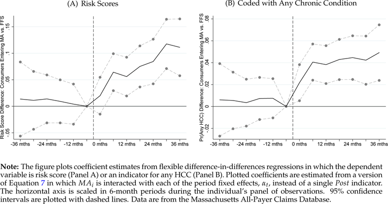
We begin in Figure 3A by plotting the coefficients from an event study version of Equation (7) where we interact MAi with each of the period fixed effects (αt) instead of a single Post indicator. This specification makes it simple to assess the existence of differential pre-trends, which here would indicate that people who would eventually choose MA were already on a path to higher risk scores prior to their actual Medicare enrollment. Each plotted coefficient represents the difference in the differences of risk scores of people entering MA vs. FFS in the indicated period relative to the period just before Medicare enrollment (period −1). The dashed vertical line indicates Medicare enrollment (the start of period 0). The figure shows that during the 36 months prior to Medicare enrollment, the risk scores for the MA and FFS groups were not differentially trending. Post-Medicare enrollment, however, there is a clear divergence, with risk scores for the MA group increasing much more rapidly than risk scores for the FFS group. By the sixth 6-month period (3 years after Medicare enrollment), normalized risk scores for the MA group were higher by a little more than 10% of the pre-period mean, relative to the FFS group. The apparent growth in the MA coding effect from time zero to 36 months is consistent with the ratcheting-up interpretation of results from column 4 of Table 2 (in the national sample and main identification strategy). These showed that effects were larger (8.7%) by the second year following a shift in θ. Figures 3B and A5 present similar event studies where the dependent variable is the probability of having any HCC during the 6-month period and the number of HCCs, respectively. These figures show similar patterns.
Figure 3:
Alternative Identification: Diff-in-Diff Event Study at Age 65, MA versus FFS
Table 5 presents regression estimates in which all 6-month periods are grouped as either pre- or post-Medicare enrollment spells, as in Equation (7). Column 1 presents results without individual fixed effects, while column 2 includes individual fixed effects, which subsume the MA indicator. The negative coefficient on MAi in the first row of column 1 indicates that during the pre-Medicare periods, people who would eventually select into MA had lower risk scores than people who would eventually select FFS, consistent with previous evidence that MA is advantageously selected (e.g., Curto et al., 2014). The coefficients of interest on MAi × Postt indicate that risk scores for the MA group grew more rapidly in the post-Medicare periods relative to the FFS group: The risk score of an individual enrolling in MA increased by 4.7 to 5.8% more than the risk score of an individual enrolling in FFS between the pre- and post-Medicare periods. This magnitude is consistent with the visual evidence in Figure 3, if one took the mean over the entire post period.
Table 5:
Alternative Identification: Coding Differences at Age 65 Threshold, MA vs. FFS
| Dependent Variable: Specification: Sample Restriction: |
Risk Score |
At least 1HCC |
Count of HCCs |
|||||||
|---|---|---|---|---|---|---|---|---|---|---|
| D-in-D Full Sample |
Matching D-in-D Full Sample |
Extensive Margin Full Sample |
Intensive Margin At least 1 HCC |
|||||||
| (1) | (2) | (3) | (4) | (5) | (6) | (7) | (8) | (9) | (10) | |
| Selected MA | −0.113** (0.007) |
−0.116** (0.006) |
−0.054** (0.005) |
−0.038** (0.005) |
−0.028** (0.005) |
−0.043** (0.003) |
−0.143** (0.014) |
|||
| Post-65 X Selected MA | 0.058** (0.009) |
0.047** (0.007) |
0.058** (0.007) |
0.054** (0.007) |
0.060** (0.007) |
0.051** (0.007) |
0.033** (0.004) |
0.033** (0.003) |
0.090** (0.018) |
0.071** (0.018) |
| Person FE | X | X | X | |||||||
| Matching Variables: | ||||||||||
| Gender/County | X | X | X | X | ||||||
| Count of HCCs | X | X | ||||||||
| Risk Score | X | X | ||||||||
| Mean of Dep. Var. | 1.00 | 1.00 | 1.00 | 1.00 | 1.00 | 1.00 | 1.00 | 0.52 | 1.07 | 1.07 |
| Observations | 319,094 | 319,094 | 316,861 | 314,293 | 288,407 | 287,676 | 319,094 | 319,094 | 118,327 | 118,327 |
Note: The table shows coefficients from difference-in-differences regressions described by Eq. 7 in which the dependent variables are the risk score (columns 1 through 6), an indicator for having at least one chronic condition (HCC) during the period (columns 7 and 8), and the count of chronic conditions, conditional on periods in which individuals have at least one HCC (columns 9 and 10). All regressions compare coding outcomes pre- and post-Medicare enrollment among individuals who select MA relative to individuals who select FFS. Data are from the Massachusetts All-Payer Claims Dataset. The unit of observation is the person-by-six month period, where six-month periods are defined relative to the month in which the individual joined Medicare. Columns 3–6 report coefficients from regressions where the observations are weighted with propensity scores estimated using the indicated matching variables. The coefficient on “Selected MA” should be interpreted as the pre-Medicare enrollment difference in the outcome for individuals who will eventually enroll in an MA plan versus individuals who will eventually enroll in FFS. The coefficient on “Post-65 X Selected MA” is the difference-in-differences coefficient. Standard errors in parentheses are clustered at the person level.
p < 0.05
p < 0.01.
The results are robust to alternative ways of controlling for MA/FFS selection. In columns 3 through 6 of Table 5, we estimate versions of the regression in column 1 in which we match individuals on pre-period observable characteristics: gender, county of residence, pre-Medicare risk scores, and pre-Medicare count of HCCs. For these regressions, we generate propensity scores on combinations of these variables, then weight the difference-in-differences regressions using these scores, dropping observations for which there is no common support. This matching procedure significantly reduces the coefficient that reflects selection: the coefficient on MAi reduces from −0.112 to −0.028. But even as the selection estimate is reduced, estimates of the difference-in-differences effect of interest (the effect of MA enrollment on risk scores in the post period) are stable, remaining similar in size to the main specifications in columns 1 and 2. In Appendix Table A9, we estimate versions of Equation (7) that include interactions between Postt and a full set of fixed effects for an individual’s pre-Medicare plan. Effects are identified off of consumers in the same pre-65 employer or individual market plan who make a different MA/FFS choice at 65. In all robustness exercises, the results are consistent with columns 1 though 6 of Table 5. Overall, these individual-level results support and complement the findings of our main analysis.
7.3. Mechanisms
In addition to the estimates of the coding effects, the richer data in the APCD allows us to investigate some of the mechanisms behind the differential coding increases we observe in MA. Of particular interest is who is upcoded: relatively healthy or relatively sick enrollees? Enrollees who, if not for MA, would not have made contact with the medical system in a given period, or enrollees with regular healthcare utilization regardless of the MA/FFS enrollment choice? Understanding such questions is useful in forming future regulatory frameworks that are less susceptible to manipulable diagnosis coding.
In columns 7 through 10 of Table 5, we investigate MA coding effects along the extensive and intensive margins. In columns 7 and 8, we replace the dependent variable with an indicator for having at least one HCC in a 6-month period. Individuals in the MA group have a lower probability of having any HCC during the pre-Medicare period, but their probability of having any HCC increases more in the post-Medicare periods relative to the FFS group. Columns 9 and 10 investigate the intensive margin. The dependent variable in these columns is the number of HCCs during the 6-month period, restricted to person-period observations with at least one HCC. We find large effects, indicating that the MA coding effect occurs on both the extensive and intensive margins.
In Appendix Table A10, we variously restrict the sample to different subsets based on pre-Medicare health status, as reflected by the diagnosed chronic conditions in the pre-Medicare employer plan. These results show that there are important effects of MA on diagnosis coding for both the healthy and the sick and that the coding effects for the sick are larger.
The (limited) healthcare utilization information in the APCD also allows us to investigate the role of healthcare use in the coding process. Table A11 presents estimates of versions of Equation 7 where we replace the dependent variable with indicators for any utilization (columns 1 and 2), any inpatient utilization (columns 3 and 4), and any non-inpatient utilization (columns 5 and 6) during a given 6month period.30 These utilization results provide novel evidence that MA has a larger positive effect on the extensive margin of healthcare utilization than FFS. At the same time, MA seems to lower the probability of having any inpatient utilization relative to FFS, though this result goes away when individual fixed effects are included. These results suggest that increasing the probability of ever seeing a doctor during a given year may be a mechanism by which MA plans achieve overall higher risk scores.
Table A12 digs further into coding mechanisms by investigating how MA affects risk scores among the set of MA and FFS enrollees who are using at least some healthcare. Specifications in Table A12 estimate versions of Equation (7) over only the 6 month periods (within individuals) for which there is positive healthcare utilization. We find that even limiting attention to enrollee-periods with non-zero utilization in MA or FFS, the post-Medicare enrollment growth in risk scores is larger in MA relative to FFS. This indicates that MA-induced differences in the probability that a patient has any contact with a medical provider in a given period (see Table A11) are not solely responsible for the differential coding observed in MA.
8. Discussion
8.1. Additional Government Spending
In the terms of Eq (5), the total additional cost of the Medicare program due to the subsidy being endogenous to risk scores is . Here we have scaled up from per capita costs to total program costs by replacing the MA share variable θMA with the count of beneficiaries, NMA. For every beneficiary choosing MA instead of FFS, total Medicare spending increases by , the base payment times the coding intensity difference.
Excess spending can be determined by combining three values: the number of MA enrollees (NMA), the average base subsidy amount paid to MA plans , and the difference between the MA and FFS risk scores (ρ). For this exercise, we use ρ = 0.064 (Table 2, column 3), though other results (Table 2, column 4 and Figure 3) suggest this estimate is likely to understate the full coding difference, which appears to ratchet up over an MA enrollment spell. We illustrate the size of the public spending impact using program parameters from 2014. In 2014, the average benchmark was $10,140 and 15.7 million beneficiaries were enrolled in an MA plan.31 Combining these values suggests that, absent any regulatory action to deflate MA plan risk scores, the additional public spending due to subsidies being endogenous to coding would have been $10.2 billion or $649 per MA enrollee.32
In fact, in 2010, toward the end of our study period, CMS began deflating MA risk scores by 3.41%, due to concerns about upcoding. In 2014, the deflation was increased to 4.91%. Factoring this adjustment into our calculations shrinks our estimate of 2014 additional public spending to about $2.4 billion, or $151 per MA enrollee that year. One could transform this accounting figure into a welfare loss given an estimate of κ, the excess burden of raising program funds.
We have generally assumed that ρ is constant across consumers or varies in a way that is uncorrelated with MA penetration. As discussed in Section 4, if instead individual-level heterogeneity in ρ were correlated with θMA, then our main results would capture coding differences only for the individuals marginal to our variation. In practice, these marginal types are likely to be close to the average MA enrollee. This is because the variation in θMA we exploit in our empirical analysis covers most of the relevant range of MA penetration, as it arises from a period of massive expansion in the MA market segment. Although individual-specific coding differences could be systematically different for FFS beneficiaries who never choose MA, our estimates reflect the parameter necessary to calculate the excess public spending, which is upcoding among MA participants.
8.2. Inefficient Sorting
In our model, MA plans can increase the subsidy they receive by over-providing services relative to the first best. This distorts consumer choices away from FFS and toward MA because MA plans pass (at least part of) these increased subsidies through to MA consumers in the form of lower premiums. Although a full analysis of the welfare costs of inefficient sorting between MA and FFS is beyond the scope of this paper, our estimates of the difference between the MA and FFS risk scores allow us to shed some light on the size of this distortion by quantifying how the size of the MA market is affected by the subsidy to more intense coding. This is related to term (ii) in Equation (5).
To estimate this quantity, we consider a counterfactual policy that uniformly deflates the risk-adjusted payments from the regulator to an MA plan to exactly compensate for the mean MA/FFS coding difference we find. Thus plans receive instead of . This change in subsidy, , can be combined with pass-through estimates and demand elasticity estimates from the literature to arrive at simulated changes in MA enrollment if the coding overpayment were removed. Pass-through describes how changes in subsidies translate to changes in consumer prices, and the demand estimates allow us to predict the impacts of these price changes on enrollment. We provide additional details of these counterfactual simulations in Appendix A.15. The results are presented in Table 6, with different MA enrollment estimates for each enrollment elasticity estimate from the literature.
Table 6:
Counterfactual: Implied MA Enrollment Effects of Removing Coding Subsidy
| Implied enrollment effect of removing overpayment due to coding |
||||
|---|---|---|---|---|
| Study | Estimated semi- price elasticity of demand |
Implied semi- payment elasticity of demand |
Relative to counterfactual of no CMS coding adjustment (6.4% reduction in payments) |
Relative to counterfactual of 3.4% coding deflation by CMS (3% reduction in payments) |
| Cabral, Geruso, and Mahoney (2014) | −0.0068 | 0.0034 | −17% | −8% |
| Atherly, Dowd, and Feldman (2003) | −0.0070 | 0.0035 | −18% | −8% |
| Town and Liu (2003) | −0.0090 | 0.0045 | −23% | −11% |
| Dunn (2010) | −0.0129 | 0.0065 | −33% | −15% |
Note: The table displays back-of-the-envelope calculations for MA market segment enrollment under a counterfactual in which the subsidy to differential coding is removed. A monthly base payment of $800 is assumed. Price semi-elasticities are taken from the prior literature. Implied semi-payment elasticities of demand have been derived from semi-price elasticities assuming a pass-through rate of 50%. See text for full details.
The back-of-the-envelope calculations in the third column of Table 6 show that modifying risk adjustment payments in this way would have large negative impacts on MA enrollment for the range of elasticities estimated in the literature. Using the smallest demand elasticity (Cabral, Geruso and Mahoney, 2017) yields a 17% decline in the size of the MA market, while the most elastic estimate (Dunn, 2010) implies a 33% decline in the size of MA under the counterfactual. These estimates of reductions in MA enrollment apply to a complete elimination of the subsidy relative to a counterfactual in which CMS did nothing to account for differential coding intensity in MA. As discussed above, toward the end of our sample period in 2010 CMS began deflating risk scores by 3.41%. In the last column of Table 6 we show the enrollment effects of increasing the CMS risk score deflation from 3.41% to the 6.4% coding difference we estimate. The estimates suggest that the additional deflation would result in a decline in MA enrollment of between 8% and 15%—a decline of 2 and 4 percentage points, respectively, based on 2010 enrollment.
Overall, upcoding has the tendency to increase MA enrollment. Relative to the first best, this decreases welfare. However, in the presence of multiple simultaneous market failures in MA, it is possible that the tendency toward over-enrollment in MA due to coding counteracts some other opposing market failure. For example, MA insurers’ market power implies markups that raise prices above marginal costs and constrain enrollment. Setting aside the distortions to MA plan benefits discussed in the next section, the enrollment effects of upcoding could thus be welfare-improving in the second best sense of counteracting market power. Of course, this offsetting relationship between “under-enrollment” in MA due to imperfect competition and “over-enrollment” in MA due to the coding subsidy would be purely coincidental. Other important market failures in this context that complicate a full welfare analysis include inertia (Sinaiko, Afendulis and Frank, 2013), spillovers between MA and FFS practice styles (Baicker, Chernew and Robbins, 2013), or the choice salience of non-cash rebates (Stockley et al., 2014). Further, the coding subsidy reinforces, rather than counteracts, the overpayment to MA plans generated by uncompensated favorable selection into MA (Brown et al., 2014).
8.3. Contract Distortions
The final component of the welfare decomposition in Equation (5) describes distortions to the MA contract itself. Our data and identifying variation do not allow us to quantify how much the observed MA contracts differ from efficient MA contracts. Nonetheless, anecdotal evidence is consistent with the idea that contract features and insurer activity are distorted in several important ways. First, there is a niche industry in MA of contractors that provide chart review services to MA carriers—searching medical records to add diagnoses that were never translated to claims. Such activity may have little direct benefit to consumers, as both the patient and their physician will often receive no feedback that their claims-listed diagnoses have changed. Public statements from the regulator, CMS, point to another example of distorted contracts in the form of in-home health assessments. These assessments in MA have drawn CMS attention because they appear aimed primarily at boosting risk scores. Such visits are often not associated with follow-up care or even communication with the primary care physician.33 Recent criminal and civil actions brought by the United States against MA organizations under the False Claims Act also allege significant insurer efforts to illegally increase risk scores using techniques that would have no clear benefits for patients.
Although we have focused on describing the insurer’s incentives for contract distortions, physician activity may also be distorted away from first best. Some MA contracts with providers tie physician payments to the risk scores the physician’s practice generates rather than to the procedures and visits performed. This can align the distortionary coding incentives between the two parties.
We speculate that the coding incentive, along with similar incentives embedded in new pay-for-performance schemes, may lead to a meaningful share of marginal investments and innovations in healthcare shifting towards the collection and processing of risk score (and other payment-focused) data for which the value to the patient is unclear at best. This cost of diagnosis-based risk adjustment must be considered when evaluating the success of these systems and the important role they play in counteracting the distortions arising from selection. Investigation of the full extent of these costs is an important area for future research.
9. Conclusion
The manipulability of the risk adjustment system via diagnosis coding is an issue of significant practical importance, given the large and growing role of risk adjustment in regulated insurance markets. Our results demonstrate wide scope for upcoding in Medicare Advantage, one of the largest risk-adjusted health insurance markets in the US, relative to the fee-for-service option. The estimates imply significant overpayments to private insurers at a cost to the taxpayer, as well as distortions to consumer choices. We also find evidence that coding intensity is increasing in a plan’s level of insurer-provider integration. Our model makes clear that even in managed competition settings such as the ACA Marketplaces—in which risk adjustment has no first-order impact on public budgets because a regulator simply enforces transfers from plans with lower average risk scores to plans with higher average risk scores—risk adjustment transfers that are endogenous to coding intensity distort the provision of coding and non-coding services offered by insurers in equilibrium.
Nonetheless, risk adjustment addresses an important problem of asymmetric information in insurance markets. Therefore, in the second best world in which adverse selection is an inherent feature of insurance markets, the optimal payment mechanism may include some kind of risk adjustment despite the costs of and distortions caused by manipulable coding. In principle, with information on the upcoding susceptibility of various conditions, it would be possible to estimate optimal payment coefficients by minimizing a loss function that included coding distortions. In practice the upcoding susceptibility of risk adjusters (especially new risk adjusters) may be difficult to observe.
One simple-to-implement improvement over the current system would be to apply one coding deflation factor to plan-reported diagnoses and a separate deflation factor to the demographic components of the risk score that originate from administrative data, such as age, sex, and disability status. Our results suggest an optimal zero deflation of the administrative portion (see Table 3) and a higher deflation to diagnoses, counter to current practice. Another potential reform applies to the audit process. Currently, CMS audits submissions of diagnoses from MA plans only for the purpose of determining whether diagnoses were legally submitted. Given that much of the upcoding we document is likely to be legal rather than fraudulent, audits that focus instead on the question of whether a given diagnosis would have been submitted under FFS could be helpful in assessing the proper deflation factors to combat overpayments. This could be done, for example, by assessing which diagnoses are established by MA plans solely via chart review (an activity that would not occur in FFS) and not captured in any claim. Such audits could help reduce the excess payments in MA, even if they would not address the marginal incentives to overcommit resources to coding.
Even with significant reform, it may not be possible to achieve perfect parity of coding intensity between the MA and FFS market segments or between competing plans within MA. In that case, any benefits of the MA program in terms of generating consumer surplus or creating cost-saving externalities within local healthcare markets should be weighed against the additional taxpayer costs and consumer choice distortions generated by a regulatory system in which the parameters determining payments are squishy.
Acknowledgments
We thank Colleen Carey, Joshua Gottlieb, and Amanda Kowalski for serving as discussants, as well as seminar participants at the 2014 Annual Health Economics Conference, the 2014 American Society of Health Economists Meeting, the BU/Harvard/MIT Health Economics Seminar, Boston University, Brigham Young University, Brown University, Chicago Booth, the Congressional Budget Office, Emory University, Harvard Medical School, the University of Illinois at Chicago, theNBERPublicEconomicsMeeting2015,UPennWharton,RAND,RTI,theSoutheasternHealthEconomicsStudyGroup, theUniversityofTexasatAustin,theUniversityofVirginia,andYaleforusefulcomments. WealsothankChrisAfendulis, Marika Cabral, Vilsa Curto, David Cutler, Francesco Decarolis, Liran Einav, Randy Ellis, Keith Ericson, Amy Finkelstein, Austin Frakt, Craig Garthwaite, Jonathan Gruber, Jonathan Kolstad, Tom McGuire, Hannah Neprash, Joe Newhouse, and Daria Pelech for assistance obtaining data and useful conversations. Layton gratefully acknowledges financial support from the National Institute of Mental Health (T32-019733). Geruso gratefully acknowledges financial support from the Robert Wood Johnson Foundation and from grants P2CHD042849, Population Research Center, and T32HD007081, Training Program in Population Studies, both awarded to the Population Research Center at The University of Texas at Austin by the Eunice Kennedy Shriver National Institute of Child Health and Human Development. Research reported in this publication was supported by National Institute of Aging of the National Institutes of Health under award number P01AG032952. The content is solely the responsibility of the authors and does not necessarily represent the official views of the National Institutes of Health.
APPENDIX. Upcoding: Evidence from Medicare on Squishy Risk Adjustment Michael Geruso and Timothy Layton
A.1. Background on MA Risk-Adjusted Payments
Medicare Advantage (MA) insurance plans are given monthly capitated payments for each enrolled Medicare beneficiary. The levels of these county-specific payments are tied to historical fee-for-service (FFS) Medicare costs in the county. County capitation rates were originally intended to capture the cost of enrolling the “national average beneficiary” in the FFS Medicare program in the county, though Congress has made many ad hoc adjustments over time.
Before 2004, there was relatively minimal risk adjustment of capitation payments in MA, relying primarily on demographics.34 In 2004, CMS began transitioning to risk adjustment based on diagnoses obtained during inpatient hospital stays and outpatient encounters. By 2007, diagnosis-based risk adjustment was fully phased-in. During our study period (2006–2011), risk-adjusted capitation payments were approximately equal to Sijc = ϕjc · xijcΛ, where i indexes beneficiaries, j indexes plans, and c indexes counties (markets).
The base payment, ϕjc, could vary within counties because since 2006 MA plans have been required to submit bids to CMS. These bids are compared to the uniform county benchmark . If the bid is below the county benchmark set by the regulator, the plan receives 75% of the difference between the bid and the benchmark, which the plan is required to fold back into its premium and benefits as a “rebate” to beneficiaries.35 Importantly for our purposes, this 75% is still paid out by CMS into the MA program. This implies that any estimation of coding subsidies should be based on the capitation payment to plans inclusive of any rebate, suggesting that the county benchmark, , is a good approximation for ϕjc.
A.2. Diagnosis Coding in Practice
Section 2.2 outlines the practices that insurers can use to influence the diagnosis coding of physicians. Here, we expand on that discussion. In Figure A1, we outline the various mechanisms insurers employ to affect diagnosis coding, and in turn risk scoring. Insights in the figure come from investigative reporting by the Center for Public Integrity, statements by CMS, and our own discussions with MA insurers and physician groups. We exclude any mechanisms that involve illegal action on the part of insurers. While fraud is a known problem in MA coding, coding differences can easily arise without any explicitly illegal actions on the part of the insurer.
First, before any patient-provider interaction even occurs, insurers can structure contracts with physician groups such that the payment to the group is a function of the risk-adjusted payment that the insurer itself receives from the regulator. This directly passes through coding incentives to the physician groups. Insurers may also choose to selectively contract with providers who code more aggressively. Additionally, the insurer can influence coding during the medical exam by providing tools to the physician that pre-populate his notes with information on prior-year diagnoses for the patient. Since risk adjustment in many settings, including MA, is based solely on the diagnoses from a single plan year, this increases the probability that diagnoses, once added, are retained indefinitely. Insurers also routinely provide training to the physician’s billing staff on how to assign codes to ensure the coding is consistent with the insurer’s financial incentives. Finally, even after claims and codes are submitted to the insurer for an encounter, the insurer may automatically or manually review claims, notes, and charts and either add new codes based on physician notes that were not originally translated to the claims or request a change to the coding in claims by the physician’s billing staff. Insurers use various software tools to scan patient medical records for diagnoses that were not recorded in originally submitted claims, but nonetheless met the statutory diagnosis eligibility requirements and can therefore be added as valid codes.
In addition to these interventions with physicians and their staffs, insurers directly incentivize their enrollees to take actions that result in more intensive coding. Insurers may incentivize or require enrollees to complete annual evaluation and management visits or “risk assessments,” which are inexpensive to the insurer, but during which codes can be added that would otherwise have gone undiscovered. Further, if an insurer observes that an enrollee whose expected risk score is high based on medical history has not visited a physician in the current plan year, the insurer can directly intervene by proactively contacting the enrollee or sending a physician or nurse to the enrollee’s home. The visit is necessary in order to code the relevant, reimbursable diagnoses for the current plan year and relatively low cost. There is substantial anecdotal evidence and numerous lawsuits related to such behavior in Medicare Advantage. See, for example, Schulte (2015).36 And regulators have expressed serious concern that such visits primarily serve to inflate risk scores. In a 2014 statement, CMS noted that home health visits and risk assessments “are typically conducted by healthcare professionals who are contracted by the vendor and are not part of the plan’s contracted provider network, i.e., are not the beneficiaries’ primary care providers.” CMS also noted that there is “little evidence that beneficiaries’ primary care providers actually use the information collected in these assessments or that the care subsequently provided to beneficiaries is substantially changed or improved as a result of the assessments.”
None of these insurer activities take place in FFS because providers under the traditional system are paid directly by the government, and the basis of these payments is procedures, not diagnoses. Under FFS, hospitals are compensated for inpatient visits via the diagnosis-related groups (DRG) payment system, in which inpatient stays are reimbursed partially based on inpatient diagnoses and partially based on procedures. It is nonetheless plausible that overall coding intensity in FFS and MA differs significantly. For one, the set of diagnoses compensated under the inpatient DRG payment system differs from that of the MA HCC payment system. In addition, the majority of FFS claims are established in the outpatient setting, in which physician reimbursement depends on procedures, not diagnoses. In FFS, diagnoses are instead used for the purpose of providing justification for the services for which the providers are requesting reimbursement.
A.3. Competitive Equilibrium with No Endogenous Risk Scores
In Section 3.3 we claim that under our model, the MA plans {δ, γ; p} offered in a competitive equilibrium mirror the parameters set by the social planner. Here we show that. Assume that the risk score is exogenous to the healthcare and coding services offered by the plan, so that the MA/FFS coding intensity difference ρ(δ, γ) is zero. Competition will lead to all insurers offering a contract that maximizes consumer surplus, subject to the zero-profit condition, or else face zero enrollment. Because consumer preferences are identical up to a taste-for-MA component that is uncorrelated with δ, γ, and costs net of risk adjustment, there is a single MA plan identically offered by all insurers. The zero profit condition here is p + S = δ + γ. The insurer’s problem, where we have substituted for price, is then
| (8) |
This produces the following first order conditions:
| (9a) |
| (9b) |
The levels of δ and γ chosen in equilibrium thus correspond precisely with the optimal levels from the social planner’s problem. Further, the zero profit condition imposes that p is equal to the social planner price that optimally allocates consumers to MA and FFS: . Thus, under the assumptions of our model, when S is exogenous to healthcare and coding, insurers offer the socially optimal contract.
Under different assumptions (i.e. preference heterogeneity correlated with cost heterogeneity not captured by the risk adjustment payments), insurers would not necessarily offer the socially optimal contract. We chose these assumptions deliberately to focus on the welfare implications of the coding distortions we study in this paper and abstract from other distortions that may also be relevant in health insurance markets but would introduce complexity that would make the coding distortions more difficult to understand.
A.4. Monopolist’s Problem with Endogenous Risk Scores
Here we show that endogenous coding distorts the monopolist’s choice of coding services, δ, and other healthcare services, γ, in the same way as in the competitive market. Using notation from Section 3.3, the monopolist’s problem is:
| (10) |
where the term on the right expresses per unit profit as price minus costs plus the subsidy that is a function of coding intensity, and θ denotes the fraction of the Medicare market choosing MA. (To better align notation with Section 3, Eq. (10) maximizes profits normalized by the size of the Medicare eligible population in the market.) This produces the following first order conditions:
| (11a) |
| (11b) |
| (11c) |
From Section 3, consumer utility net of premiums is , where σ is distributed F(·). Noting that and defining , we rewrite as . We similarly rewrite as and as . This allows us to simplify the conditions to:
| (12a) |
| (12b) |
| (12c) |
The conditions determining the levels of δ and γ are identical to those in the competitive equilibrium. The intuition behind the robustness of this result to the imperfect competition case is that if an insurance carrier can pay a chart review contractor $1.00 to mine diagnosis codes that generate $1.50 in risk adjustment revenues, they should be expected to do so regardless of market structure.
Prices differ from the competitive equilibrium by a standard absolute markup term. The monopolist sets prices equal to (net) marginal costs plus a markup that is inversely related to the semi-elasticity of demand with respect to price. With infinite elasticity residual demand, the pricing condition simplifies to the competitive equilibrium price.
If contrary to our model’s assumptions, the utility function had non-zero cross derivatives with respect to coding services and premiums, so that the marginal consumer utility generated by an insurer’s coding activities covaried with the level of premium paid by the consumer, then the equivalence between the competitive market coding intensity and the monopolist coding intensity would no longer hold. In this case, the level of coding services would be a function of the premium prices (which vary with the level of competition).
A.5. Derivation of Expression 5
Welfare is the social surplus generated for enrollees in each of the MA and FFS market segments minus the distortionary cost of raising public funds to subsidize (both segments of) the market. To express welfare, let θMA and θFFS denote the fraction of the Medicare market enrolled in the MA and FFS segments, respectively. Let ΦMA and ΦFFS tally the per-enrollee social surplus generated by each option, excepting the idiosyncratic taste component, σ. Enrollment and surplus in the FFS and MA segments are:
| (13a) |
| (13b) |
| (13c) |
| (13d) |
Following these variable definitions, the competitive equilibrium social surplus per capita for the case of endogenous risk scores that affect plan subsidies is
| (14) |
The competitive equilibrium social surplus per capita for the case of risk scores that do affect plan subsidies, and in which first best levels of coding and healthcare services are provided is
| (15) |
Note that in the case of Expression 15, the excess burden term reduces to because MA by construction costs the same as FFS, and so costs don’t vary with MA penetration, θMA. The difference between and WExo can be written:
| (16) |
| (17) |
| (18) |
which reduces to:
| (19) |
| (20) |
A.6. Further Discussion of Complete Coding and Socially Efficient Coding
In Section 3.4 we argue that “complete” coding is not a useful benchmark for welfare as “complete” coding ignores the social resource costs of the coding. A more useful alternative benchmark would be the difference between the equilibrium level of coding services and the socially efficient level (δ∗). We cannot observe this, given that our data contain no information on the marginal costs of providing coding-related services, and given that our identifying variation is keyed to recovering coding differences rather than recovering consumer valuations over various healthcare services. We view understanding the socially efficient level of diagnosis coding as an important avenue for future research. In particular, this would be informative as to the size of the third source of inefficiency from Equation (5), inefficient contract design.
A.7. Identifying Coding Differences Via the Market Average Risk Score Curve
In Section 4 we claim that the slope of the market average risk score with respect to MA penetration identifies a FFS/MA coding difference. Here we provide proofs and extensions. We begin with the case of an additively separable coding effect and then proceed to an alternative data generating process that involves multiplicative effects. For each case, we discuss the implications if individual heterogeneity in differential coding is correlated with θ.
Define the risk score an individual would have received in FFS as . Define the same person’s risk score had they enrolled in MA as the sum of this FFS risk score, a mean MA/FFS difference ρ and an arbitrary person-level shifter: . The ϵi term is mean zero ( removes the mean), but can vary arbitrarily to capture individual-level heterogeneity in the tendency to produce a different risk score in MA relative to FFS. Let denote an indicator function for i choosing MA. An individual’s risk score as a function of MA enrollment is then . The county-level mean risk score as a function of MA enrollment is analogously
| (21) |
where expresses the unconditional expectation of and the integral captures the average MA/FFS coding difference among MA enrollees when the MA share equals θMA. Here ϵ(θ) describes the epsilon of the consumer type that is on the FFS/MA margin at some θ. (Any variation in ei that is orthogonal to θ will not impact the derivative of interest.) Small changes in θ identify
| (22) |
where the latter equality follows from the Leibniz rule. Thus, the slope of the market average risk score identifies the coding difference for types just indifferent between MA and FFS. If within this group there is heterogeneity in ϵi, the slope identifies plus the the mean of epsilon among these marginal types. We illustrate the idea in Figure A6. The figure shows how the slope of the market average risk curve varies when is a function of θ. Note that if is not a function of θ then the slope of the market average risk curve is constant across all levels of θ and equal to . If susceptibility to differential coding intensity varies across consumers in a way that is correlated with MA market share, then the market-level average risk curve will be nonlinear, as this curve integrates over the varying e. In the case that e varies in θ, then is non-linear, and small changes in θ identify the MA/FFS coding difference among consumers on the MA/FFS margin. The estimate of the coding effect is exact for types at the margin, but may not be representative for types away from the identifying variation in θ.
Note that because ϵi is allowed to be arbitrary, we have made no assumption on the distribution of or on the joint distribution of risks and preferences that generate the within-market segment average risk curves that describe selection ( and ). As we describe in Section 4, this result simplifies to if individual heterogeneity in the tendency to be differentially coded is orthogonal to θ.
These proofs hold for small variations in θ. In practice, we estimate using larger, discrete changes in θ. As discussed above, in this case the slope of the market average risk curve is equal to plus the mean of epsilon among the types whose FFS/MA choice is marginal to the empirical variation in θ used to estimate the slope. This can be seen in Figure A6. In the figure, the market average risk curve (the red line) is assumed to be concave (we find some evidence that in practice). The dashed line indicates the coding intensity difference for the marginal person at the indicated level of . The figure indicates that the slope of the market average risk curve is equal to this coding intensity difference at any given level of θ.
It now seems prudent to ask what is the parameter of interest here, the marginal or the average coding intensity difference. This depends on the question being asked. For example, one might be interested in knowing how much risk scores would increase if MA penetration went from 0% to 100%. In this case, the average coding intensity difference across the entire population (ρ) would be the parameter of interest. On the other hand, one might be interested in knowing how much risk scores would decrease if MA risk scores were equal to FFS risk scores. Here, the average coding intensity difference across the set of individuals enrolled in MA would be the parameter of interest. Note that in the case where heterogeneity in coding intensity is orthogonal to θ, these two parameters are equivalent. However, in the more general case, they may differ. To see this, let us return to Figure A6. In the figure, the dotted line indicates the average coding intensity difference for the set of individuals enrolled in MA for each level of θ. The line is defined on the left y-axis (0% MA market share) by the coding intensity difference for the first individual to enroll in MA. It is defined on the right y-axis (100% MA market share) by the average coding intensity across the entire population, which in this case is equal to 0.07. Now, assume that in reality θ = 0.35 so that 35% of beneficiaries are enrolled in MA. At this level of θ, the market average risk score is 1.04, the marginal coding intensity difference is 0.09, and the average coding difference among the individuals enrolled in MA is 0.11. Unlike the orthogonal heterogeneity case, these values clearly differ. Now, recall that our estimate of the slope of the market average risk curve depends on the range of θ used to empirically estimate the slope. If we observe variation in θ spanning from θ = 0 to θ = 0.35, then we would estimate a slope of , the average coding difference among the individuals enrolled in MA. This is not a coincidence: The estimated slope of the market average risk curve will always approximate the average coding difference among the set of individuals whose MA/FFS choice is marginal to the variation in MA. This is true for any arbitrary heterogeneity in the coding intensity difference.
Finally, we explore the case where plan coding effects multiply individual risk score components, rather than adding to these. Here, the coding factor can similarly be derived from the slope . Consider a data generating process in which as above, but , where d > 1 would correspond to higher MA coding intensity. Defining , an individual’s risk score as a function of MA enrollment is . The county-level mean risk score as a function MA enrollment is
| (23) |
where expresses the unconditional expectation of . Here ϵ(θ) describes the epsilon of the consumer type that is on the FFS/MA margin at some θ. (Any variation in ϵi that is orthogonal to θ will not impact the derivative of interest.) Small changes in θ identify
| (24) |
In this case, the slope of the market average risk score identifies the coding difference for types just indifferent between MA and FFS, multiplied by the mean FFS risk score of these marginal types, . Again this result simplifies if individual heterogeneity in the tendency to be differentially coded is orthogonal to θ. In that case, . In practice, the FFS risk scores of the marginal types appear to not vary in θ and are very close to 1.0. In a cross-county regression of mean FFS risk scores on MA share of the form , we estimate α = 0.975 and β = .058. Thus even over a wide range of θ, there is very little variation in cross-county means of FFS risk scores (corresponding to in the model). To put this in context, these parameters imply that while . These are small differences. That these averages don’t vary systematically with θ suggests that the marginals likewise do not strongly covary with θ. Because in practice, county-level means of appear to be very close to one, is approximately without additional adjustment.
A.8. Data Notes: County-Level MA Data
Here we provide some additional notes on the risk score data described in Section 5 of the paper:
The RAPS dataset includes risk scores for every Medicare enrollee, both those enrolled in MA and those enrolled in FFS. The FFS risk scores are constructed by CMS using diagnoses found in FFS claims data. The MA risk scores are constructed by CMS using diagnoses submitted to the RAPS by individual MA plans. These diagnoses may or may not appear on MA claims data, as some diagnoses are extracted directly from physician notes instead of from claims. Similar data are unavailable before 2006, since diagnosis-based risk scores were not previously generated by the regulator.
In constructing county-level risk scores, we exclude only enrollees in the Program of All-inclusive Care for the Elderly (PACE) plans.
CMS has not traditionally provided researchers with individual-level risk scores for MA enrollees (two exceptions are Brown et al. (2014) and Curto et al. (2014)). A strength of our identification strategy, which could easily be applied in other settings like Medicaid Managed Care and Health Insurance Exchanges, is that it does not require individual-level data.
The regulator’s algorithm specifies that the demographic components and diagnostic components of individual risk scores are additively separable, which implies that the county averages are also additively separable: . This is useful in a falsification test in which we examine “effects” of shifting MA penetration on the demographic portion of the risk score.
A.9. Estimates of Selection
Section 6 describes the results of the main analysis in which we regress county-level averages of risk scores on lagged MA penetration in the county to estimate coding differences. For completeness, here we estimate selection on risk scores, using an analogous set of regressions. Under the assumption that MA penetration changes are exogenous to changes in underlying population health conditional on our controls, selection on risk scores can be estimated by regressing either the average risk score within FFS or the average risk score within MA on contemporaneous and lagged penetration. Note that this reveals only compensated selection, not uncompensated selection as estimated in Brown et al. (2014) and Cabral, Geruso and Mahoney (2017).
Table A13 presents the selection results. Coefficients on contemporaneous MA penetration identify pure selection effects. If selection were monotonic (such as in Figure 1), then positive contemporaneous coefficients in both markets would indicate that as penetration increased, the marginal beneficiary choosing MA was high risk relative to the MA average and low risk relative to the FFS average (according to prior-year diagnoses), increasing the average risk score in both pools. In Table A13, estimates for both FFS and MA risk are imprecise, yielding confidence intervals consistent with a broad range of selection effects, including the findings in Newhouse, et al. (2012)37 of advantageous selection into MA of 4 to 9% of the risk score in 2008.
An important component of selection effects may be captured by the lagged penetration coefficient: Research on MA enrollment by Sinaiko, Afendulis and Frank (2013) shows that many of new MA enrollees are age 65, implying that at least some portion of the shift in MA penetration is likely occurring among the newly Medicare-eligible. In Table A13, this would cause a significant fraction of selection effects to be captured by the lagged coefficient, as new MA enrollees aren’t assigned diagnosis-based risk scores until their second year. However, interpreting selection effects in Table A13 is difficult because coefficients on lagged MA penetration are affected by: (i) selection on risk score trajectory and (ii) selection on the unobserved contemporaneous risk score for new enrollees who are not assigned a diagnosis-based score until their second year.
It is important to note that unlike these within-market-segment results, the regressions comprising our main analysis, which examine the effect of lagged penetration on overall county risk, are unaffected by selection and yield a straightforward identification of pure coding effects.
A.10. Supplemental Analysis on Plan Ownership
In Section 6 we described results that identified heterogeneity in coding practices across plans with different levels of insurer-provider integration. For our results in column (5) of Table 4, we calculated MA penetration separately for provider-owned plans, using data constructed by Frakt, Pizer and Feldman (2013). Here, we describe those data and results in more detail.
Frakt, Pizer and Feldman (2013) gathered data on provider ownership of plans via plan websites and governance documents for plan year 2009. They limited attention to coordinated care MA-Part D plans (e.g. HMOs and PPOs), excluding employer plans, PFFS plans, and MA plans without drug coverage. We apply their integration flag to our data covering years 2006–2011, using publicly available CMS plan crosswalk files to link the 2009 plan IDs across years. The restriction of Frakt, Pizer and Feldman (2013) to exclude non-drug plans from classification and our implicit assumption that physician ownership was constant from 2006 to 2011 could introduce measurement error, which would bias against our finding of a difference in coding between plans classified as provider-owned and not.
A.11. The Role of Electronic Health Record (EHR) Adoption
We investigate the possibility that EHR adoption affects coding intensity using data on adoption of EHR by office-based physicians. CMS, in cooperation with the Office of the National Coordinator for Health Information Technology, has collected data on meaningful use of EHR systems within physician office settings at the county level. Since 2011, physician offices serving Medicare patients have been incentivized with financial bonuses to report on meaningful EHR use to CMS. We use reports of EHR use during the first year of the incentive program (2011) as a proxy for the existing local EHR infrastructure during our sample period (2006–2011). Within each county, we normalize the count of physicians reporting office EHR adoption by the county Medicare population. Then we define an indicator for high EHR adoption by splitting this metric at the median.
Regressions in Table A6 analyze the extent of coding intensity differences across markets classified by differences in the local adoption of electronic health records (EHRs). Interaction terms in Table A6 between lagged penetration and this indicator for high EHR adoption yield coefficients very close to zero, though the standard errors do not rule out small effects.
A.12. Heterogeneity by For-Profit Status
We classified HMO and PPO plans into three mutually exclusive categories by first partitioning plans into a group including national and large regional carriers and a second group capturing smaller, local organizations. The group of national and large regional plans included, for example, plans offered by Aetna, United Health Group, Blue Cross Blue Shield, and Kaiser. These made up about two-thirds of the enrollee-years in our sample. Smaller organizations included, for example, the Rochester Area Health Maintenance Organization and Puget Sound Health Partners, Inc. We further divided the national and large regional MA carriers by their for-profit/not-for-profit status.
To investigate possible heterogeneity in coding intensity across plans of different for-profit statuses, we generated separate MA market share variables measuring the for-profit and not-for-profit plans and included these as separate regressors in a regression that also included the overall MA share. Table A7 presents the results. Because “main effects” for overall MA penetration are included in each regression, the coefficients on the for-profit and not-for-profit share variables can be interpreted as interaction terms that measure the difference in coding intensity for the indicated type of MA plan, relative to the excluded plan category. Column 1 compares for-profits to an excluded group comprised of not-for-profits and local plans. Column 2 compares not-for-profits to an excluded group comprised of for-profits and local plans. Column 3 estimates separate coefficients for for-profits and not-for-profits relative to local plans.
The table shows no evidence of differential coding intensity across profit status, or across local versus regional and national plans. Note that while the standard errors on the interaction terms are large enough to potentially mask some heterogeneity, the point estimates for the effect of overall MA penetration are very stable across the additions of profit status controls in columns 1 through 3 (0.063, 0.064, and 0.062). These can be compared to the main coefficient estimate of 0.064 from Table 2.
A.13. Data Notes: Massachusetts All-Payer Claim
Here we provide some additional notes on the data described in Section 7.1 of the paper:
The Massachusetts All-Payer Claims Dataset (APCD) includes records for 2009 through 2013. We exclude 2009 due to irregularities in the data.
For FFS enrollees with supplemental Medigap coverage, Medigap pays some fraction of almost every FFS claim, creating a duplicate record of the information in the FFS claim sent to Medicare in the form of a Medigap claim we can observe. Nationally, about 31% of 65-year-old FFS enrollees have a supplemental Medigap policy. The only claims that Medigap does not pay any part of are hospital readmissions and lab claims (paid in full by FFS). Our analysis assumes these types of claims contain no relevant diagnoses that are not also recorded on another claim for the beneficiary. For hospital readmissions, it is unlikely that the new admission will include relevant diagnoses of a chronic condition that did not appear in a prior admission. Differential treatment of lab claims is irrelevant for the calculation of risk scores because the CMS algorithm that generates HCCs from claims ignores diagnoses recorded on lab claims. Conditional on the FFS enrollee having a Medigap plan, we observe a complete record of all the diagnosis information needed to construct a risk score. To the extent that our sample of observable FFS enrollees is a good proxy for the full FFS population in Massachusetts with respect to changes in coding at age 65, we can estimate the differential change in diagnoses at 65 among MA enrollees relative to FFS enrollees. Note that this requirement is weaker than requiring that levels of risk scores are similar between FFS enrollees with and without Medigap.
We drop any individual who is enrolled in both MA and Medigap post-Medicare enrollment, either contemporaneously or at different points in time so that our MA and Medigap groups are mutually exclusive. For each individual, we construct a panel of health insurance enrollment at the level of the 6-month period relative to the month in which the individual enrolled in Medicare.
In sample construction, for the pre-Medicare period we include all 6-month periods during which the individual was continuously enrolled in some form of health insurance except for 6month periods prior to a gap in coverage. For the post-Medicare period, we include all 6-month periods during which the individual was continuously enrolled in either MA or Medigap except for 6-month periods after a gap in coverage.
We assume that the set of Medigap FFS enrollees we observe is a good proxy for the full FFS population in Massachusetts with respect to changes in coding at age 65. This requirement is weaker than requiring that levels of risk scores are similar between FFS enrollees with and without Medigap. FFS enrollees with Medigap and FFS enrollees without Medigap are unlikely to experience different changes in coding upon enrollment in Medicare. This is because Medigap plans, unlike MA plans, solely reimburse cost-sharing for services and do not engage in care management or steer patients to a particular set of providers. Nonetheless, a mechanism by which Medigap could influence coding in principle is by increasing an enrollee’s utilization of health care (via a demand response to net price). This could lead to more provider-patient encounters during which codes could be obtained. Though we expect such effects are ignorably small, such a phenomenon would imply our estimates of FFS-MA coding differences below are biased toward zero: This type of demand response to Medigap would imply that the increase in FFS risk scores at age 65 in our sample overstates the average change in risk scores in FFS overall. This implies that our estimates of the differential change in coding in MA relative to FFS would be a lower bound of the true differential change.
A.14. Practice Style Spillovers in Equilibrium
It is possible that the presence of MA in a market affects how FFS enrollees in the same market are coded—perhaps because the same physicians treat patients from both regimes. In the context of the model, spillovers that brought FFS coding closer to MA coding would decrease the excess cost of MA, as only the MA/FFS coding difference matters for the public funds term of Equation (5). But such convergence could nonetheless exacerbate the inefficient attention paid to coding, extending it beyond MA plans.
With respect to our estimates, if coding practice spillovers varied as a function of MA penetration, then our market-level estimates in Section 6.1 would not accurately capture the difference between MA scores and counterfactual FFS scores.38 The estimates would still estimate the causal effects of MA on county-level risk scores, but the interpretation would change, as the coefficients would be influenced both by MA/FFS coding differences and by any changes to FFS coding that resulted from higher MA penetration. This potential complication arises because the national analysis is identified off of changes in the local MA presence.
The person fixed-effects analysis, however, does not share this property. In the years leading up to our sample period for the Massachusetts analysis, MA plan presence in Massachusetts was remarkably stable: MA penetration in Massachusetts declined by an insignificant 0.2 percentage points from 2008 to 2011. This implies that any coding practice spillovers from MA to FFS are likely to have already occurred and that the coding differences we estimate using the person-fixed effects strategy fully captures equilibrium MA vs. FFS coding intensity differences, net of such spillovers. The person fixed-effects results thus represent a test of whether our estimates from Section 6.1 are overestimates of the longer run MA/FFS coding difference due to spillovers of MA coding practices to FFS. Because the estimated coding differences are very similar under the two identification strategies, this test provides evidence—consistent with beliefs and action by regulators—that FFS coding practices are not merely converging to MA coding practices over time.
A.15. MA Enrollment Counterfactuals
To estimate the effects of reducing the subsidy to MA plans by the amount of the coding subsidy implied by our estimates, we consider a counterfactual policy that uniformly deflates the risk-adjusted payments from the regulator to an MA plan to exactly compensate for the mean MA/FFS coding difference we find. Thus plans receive instead of . This change in subsidy, , can be combined with demand elasticity estimates from the literature to arrive at simulated changes in MA enrollment if the coding overpayment were removed.
Using program parameters that correspond approximately to 2010, the transition year in whichCMS began deflating risk scores, we assume a monthly base capitation payment of . Drawing on the 6.4% estimate from Table 2, column 3, the simulated change in monthly payment is $51 (= 0.064 · $800). Most previous studies of MA demand have estimated semi-elasticities with respect to the consumer premium , where p equals the consumer premium and θ denotes the MA market segment enrollment, as above. Table 6 reports these demand elasticities from the literature. The parameter needed for generating the relevant counterfactuals is the elasticity of demand for the MA market segment with respect to subsidy payments to MA plans, . We convert plan price semi-elasticities to plan payment semi-elasticities using empirical estimates of the pass-∂p through rate, . The pass-through rate expresses how the marginal government payment to MA plans translates into lower premiums or higher rebates for consumers. Theory predicts that under perfect competition and assuming no selection on enrollee net cost, this parameter would equal −1, as competition forces premiums down dollar-for-dollar with the increased subsidy. Unlike in the stylized model of Section 3, we allow here for imperfect competition, which dampens the enrollment effects of upcoding if pass-through are less than 1 in absolute value. Several studies, including Song, Landrum and Chernew (2013)39, Cabral, Geruso and Mahoney (2017), and Curto et al. (2014), find pass-through rates in MA of about 50%.40 We therefore assume 50% pass-through. Results are presented in Table 6.
Figure A1:

How Risk Scores are Influenced by Insurers
Figure A2:
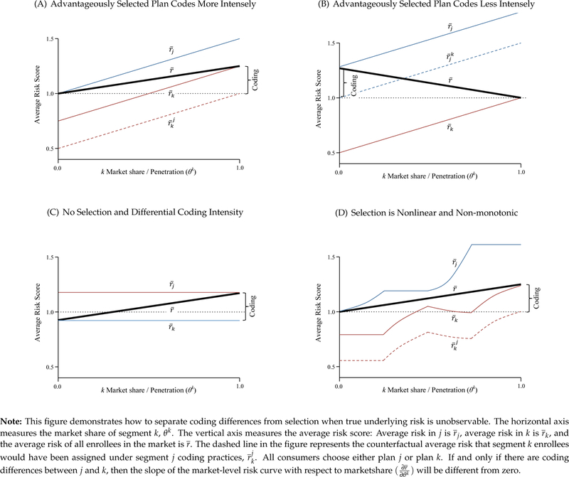
Identifying Coding Differences in Selection Markets: Alternative Forms of Selection
Figure A3:
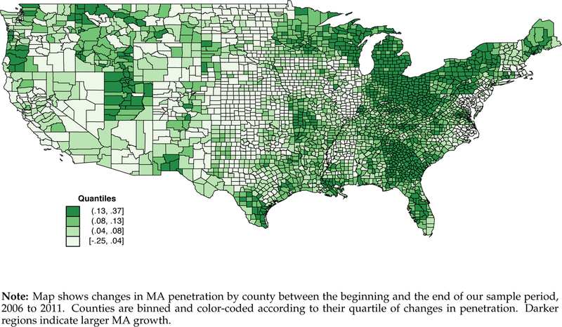
Geography of Growth in Medicare Advantage, 2006 to 2011
Figure A4:
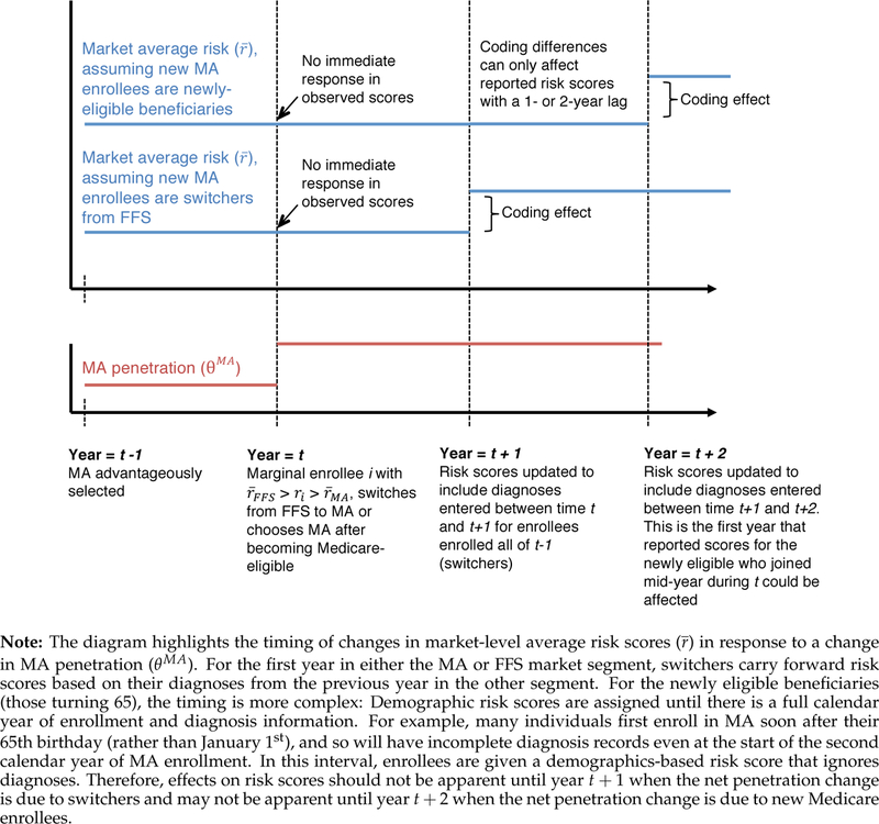
Identification: Coding Effects Plausibly Observed Only with a Lag in Medicare
Figure A5:
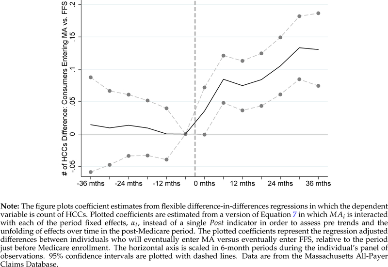
Diff-in-Diff Event Study at Age 65: Counts of Coded Conditions
Figure A6:
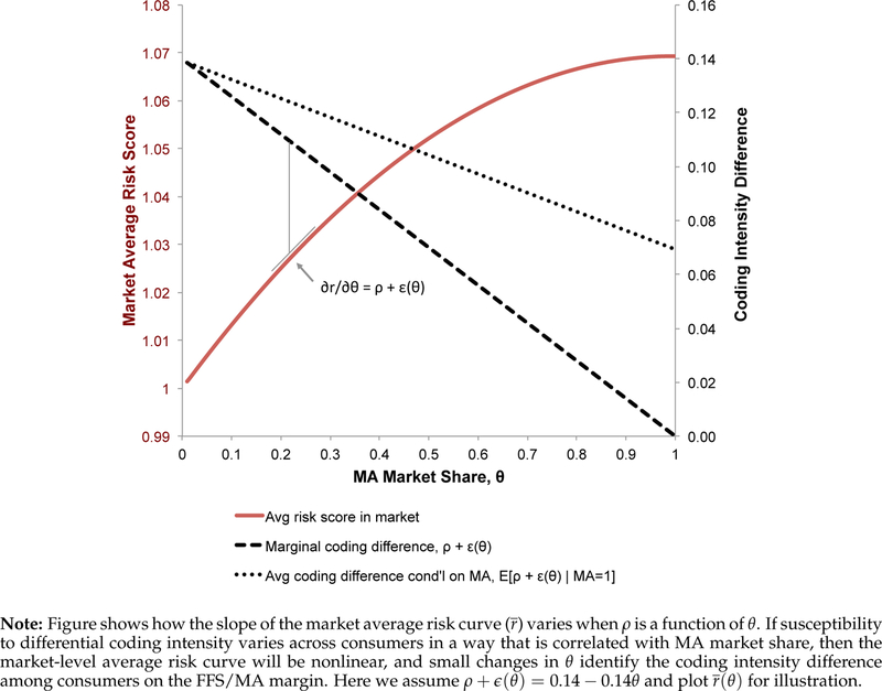
Identification when ρ+ϵ Varies with θ
Table A1:
Results with Non-Normalized Risk Scores
| Dependent Variable: County-Level Average Risk Score | ||||||
|---|---|---|---|---|---|---|
| Normalized Dependent Variable (Main Specification) |
Non-Normalized Dependent Variable | |||||
| (1) | (2) | (3) | (4) | (5) | (6) | |
| MA Penetration t (placebo) | 0.007 (0.015) |
0.001 (0.019) |
0.001 (0.019) |
0.016 (0.016) |
0.004 (0.020) |
0.004 (0.020) |
| MA Penetration t-1 | 0.069** (0.011) |
0.067** (0.012) |
0.064** (0.011) |
0.070** (0.011) |
0.068** (0.012) |
0.066** (0.012) |
| Main Effects | ||||||
| County FE | X | X | X | X | X | X |
| Year FE | X | X | X | X | X | X |
| Additional Controls | ||||||
| State X Year Trend | X | X | X | X | ||
| County X Year Demographics | X | X | ||||
| Mean of Dep. Var. | 1.00 | 1.00 | 1.00 | 1.03 | 1.03 | 1.03 |
| Observations | 15,640 | 15,640 | 15,640 | 15,640 | 15,640 | 15,640 |
Note: The table reports coefficients from difference-in-differences regressions in which the dependent variable is the average risk score in the market (county). Effects of contemporaneous (t) and lagged (t − 1) Medicare Advantage (MA) penetration are displayed. Columns 1 through 3 repeat specifications in Table 2 for comparison. Columns 4 through 6 use a non-normalized version of the risk score as the dependent variable, rather than normalizing so that the national average is exactly 1.0 in each year. Additional controls are as described in Table 2. Observations are county × years. Standard errors in parentheses are clustered at the county level.
p < 0.05
p < 0.01.
Table A2:
Robustness to Additional Time Varying County Controls
| Dependent Variable: County-Level Average Risk Score | |||||||||
|---|---|---|---|---|---|---|---|---|---|
| (1) | (2) | (3) | (4) | (5) | (6) | (7) | (8) | (9) | |
| MA Penetration t (placebo) | 0.001 (0.019) |
−0.004 (0.019) |
0.001 (0.018) |
−0.004 (0.019) |
0.009 (0.034) |
0.001 (0.019) |
0.002 (0.021) |
0.001 (0.019) |
−0.008 (0.039) |
| MA Penetration t-1 | 0.064** (0.011) |
0.064** (0.011) |
0.062** (0.012) |
0.061** (0.011) |
0.077** (0.022) |
0.064** (0.011) |
0.067** (0.011) |
0.063** (0.011) |
0.082** (0.022) |
| Main Controls | |||||||||
| County FE | X | X | X | X | X | X | X | X | X |
| Year FE | X | X | X | X | X | X | X | X | X |
| State X Year Trend | X | X | X | X | X | X | X | X | X |
| County X Year Demographics | X | X | X | X | X | X | X | X | X |
| Extended Controls (county-by-year) | |||||||||
| Medicare Enrollees | X | X | |||||||
| ln(Medicare Enrollees) | X | X | |||||||
| Share Dual Eligible | X | X | |||||||
| Share Enrolled in Employer MA | X | X | |||||||
| Share <65 (Newly Disabled, Proxy) | X | X | |||||||
| Fraction FFS ESRD | X | X | |||||||
| Share Enrolled in SNP Plans | X | X | |||||||
| Observations | 15,640 | 15,640 | 15,640 | 15,640 | 15,640 | 15,640 | 15,640 | 15,640 | 15,640 |
Note: The table reports coefficients from difference-in-differences regressions in which the dependent variable is the average risk score in the market (county). Effects of contemporaneous (t) and lagged (t − 1) Medicare Advantage (MA) penetration are displayed. Columns add time varying county-level controls as indicated. Column 6 controls for the share of Medicare enrollees who are under age 65 in the county-year to proxy for changes in county-level prevalence of disability-eligible Medicare beneficiaries. Column 7 controls for the fraction of the FFS population with end-stage renal disease. Main controls are as described in Table 2. Observations are county × years. Standard errors in parentheses are clustered at the county level.
p < 0.05
p < 0.01.
Table A3:
Results with Weighting and Trimming
| Panel A: Weighting by Ln(County Medicare Population) | |||
|---|---|---|---|
| (1) | (2) | (3) | |
| MA Penetration t-1 | 0.068** (0.009) |
0.063** (0.010) |
0.060** (0.010) |
| Observations | 15,640 | 15,640 | 15,640 |
| Panel B: Dropping Smallest Counties, by Medicare Population Size | |||
| Trimming < 1 percentile | Trimming < 5 percentile | Trimming < 10 percentile | |
| (4) | (5) | (6) | |
| MA Penetration t-1 | 0.065** (0.010) |
0.060** (0.009) |
0.059** (0.009) |
| Observations | 15,480 | 14,855 | 14,075 |
| Panel C: Dropping Largest and Smallest Counties, by Medicare Population Size | |||
| Trimming < 1 & >99 percentile | Trimming < 5 & >95 percentile | Trimming < 10 & >90 percentile | |
| (7) | (8) | (9) | |
| MA Penetration t-1 | 0.067** (0.010) |
0.065** (0.010) |
0.064** (0.010) |
| Observations | 15,320 | 14,070 | 12,510 |
| Main Effects | |||
| County FE | X | X | X |
| Year FE | X | X | X |
| Additional Controls | |||
| State X Year Trend | X | X | |
| County X Year Demographics | X | ||
Note: The table reports coefficients from difference-in-differences regressions in which the dependent variable is the average risk score in the market (county). Effects of lagged Medicare Advantage (MA) penetration are displayed. Contemporaneous effects are included in regressions but supressed for readability. Panel A weights the regression by the natural log of the size of the county Medicare population. Panel B drops the smallest 1%, 5%, or 10% of counties, by Medicare population size. Panel B drops the smallest and largest 1%, 5%, or 10% of counties, by Medicare population size. Controls are as described in Table 2. Observations are county × years. Standard errors in parentheses are clustered at the county level.
p < 0.05
p < 0.01.
Table A4:
Extended Placebo Tests: Effects of Contemporaneous Penetration and Leads
| Dependent Variable: County-Level Average Risk Score | ||||||||
|---|---|---|---|---|---|---|---|---|
| available panel years: | 2007–2011 | 2007–2010 | 2007–2009 | 2008–2011 | 2008–2010 | 2008–2009 | 2009–2011 | 2009–2010 |
| (1) | (2) | (3) | (4) | (5) | (6) | (7) | (8) | |
| MA Penetration t+2 (placebo) | 0.044 (0.023) |
0.030 (0.036) |
||||||
| MA Penetration t+1 (placebo) | 0.017 (0.025) |
0.032 (0.056) |
−0.005 (0.015) |
−0.019 (0.042) |
−0.004 (0.034) |
|||
| MA Penetration t (placebo) | 0.001 (0.019) |
−0.021 (0.028) |
−0.064 (0.071) |
0.006 (0.017) |
0.003 (0.025) |
−0.025 (0.091) |
0.011 (0.016) |
0.014 (0.043) |
| MA Penetration t-1 | 0.064** (0.011) |
0.076** (0.018) |
0.084** (0.022) |
0.041** (0.015) |
0.038 (0.022) |
0.025 (0.038) |
0.037 (0.032) |
0.052 (0.090) |
| MA Penetration t-2 | 0.046* (0.022) |
0.054* (0.024) |
0.048 (0.041) |
0.052 (0.031) |
0.100 (0.061) |
|||
| MA Penetration t-3 | 0.023 (0.024) |
−0.033 (0.039) |
||||||
| Main Effects | ||||||||
| County FE | X | X | X | X | X | X | X | X |
| Year FE | X | X | X | X | X | X | X | X |
| Additional Controls | ||||||||
| State X Year Trend | X | X | X | X | X | X | X | X |
| County X Year Demographics | X | X | X | X | X | X | X | X |
| Observations | 15,640 | 12,512 | 9,384 | 12,512 | 9,384 | 6,256 | 9,384 | 6,256 |
Note: The table shows coefficients from difference-in-differences regressions in which the dependent variable is the average risk score in the market (county). Effects of future (t + 2, t + 1), contemporaneous (t), and lagged (t − 1, t − 2, t − 3) Medicare Advantage (MA) penetration are displayed. Because MA risk scores are calculated using diagnosis data from the prior plan year, changes in MA enrollment can plausibly affect reported risk scores via differential coding only with a lag. See Figure A4 for details of this timing. Contemporaneous penetration and leads of penetration serve as placebos that allow for tests for pre-trends within the county. The data include penetration from 2006 through 2011 and market risk from 2007 through 2011. The inclusion of leads and lags determines the available panel years, listed in the header for each column. Observations are county × years. Controls are as described in Table 2. Standard errors in parentheses are clustered at the county level.
p < 0.05
p < 0.01.
Table A5:
Falsification Test: Effects on Medicare Age Distribution
| Dependent: Variable: Fraction ≥65 |
Dependent Variable: Indicator for Age Bin, Conditional on ≥65 |
|||||
|---|---|---|---|---|---|---|
| 65–69 | 70–74 | 75–79 | 80–84 | 85+ | ||
| (1) | (2) | (3) | (4) | (5) | (6) | |
| MA Penetration t | 0.006 (0.005) |
0.002 (0.007) |
0.008 (0.007) |
−0.004 (0.006) |
−0.001 (0.006) |
−0.006 (0.003) |
| MA Penetration t-1 | 0.003 (0.004) |
−0.006 (0.006) |
0.019** (0.006) |
−0.006 (0.007) |
−0.003 (0.006) |
−0.004 (0.004) |
| Main Effects | ||||||
| County FE | X | X | X | X | X | X |
| Year FE | X | X | X | X | X | X |
| Additional Controls | ||||||
| State X Year Trend | X | X | X | X | X | X |
| County X Year Demographics | ||||||
| Observations | 15,640 | 15,640 | 15,640 | 15,640 | 15,640 | 15,640 |
Note: The table shows coefficients from difference-in-differences regressions in which the dependent variables are indicators for age ranges. The dependent variable in column 1 is the fraction of the Medicare population with age ≥ 65. The dependent variables in columns 2 through 6 are the fractions of the Medicare population in the indicated age bins, conditional on age ≥ 65. Data on the Medicare age distribution come from the Medicare Beneficiary Summary File. Observations are county × years. Controls are as described in Table 2. Standard errors in parentheses are clustered at the county level.
p < 0.05
p < 0.01.
Table A6:
No Coding Interaction with Electronic Health Records
| Dependent Variable: County-Level Average Risk Score |
|||
|---|---|---|---|
| (1) | (2) | (3) | |
| MA Penetration t-1 | 0.069** (0.016) |
0.069** (0.017) |
0.066** (0.016) |
| High HER X MA Penetration t-1 | −0.001 (0.018) |
−0.004 (0.017) |
−0.005 (0.017) |
| Main Effects | |||
| County FE | X | X | X |
| Year FE | X | X | X |
| Additional Controls | |||
| State X Year Trend | X | X | |
| County X Year Demographics | X | ||
| Observations | 15,640 | 15,640 | 15,640 |
Note: The table shows coefficients from difference-in-differences regressions in which the dependent variable is the average risk score in the market (county). Effects of lagged (t − 1) Medicare Advantage (MA) penetration are displayed. Contemporaneous effects are included in regressions but supressed for readability. Regressions include interactions between the MA penetration variables and an indicator for high electronic health record (EHR) adoption by physician offices in the county. Data on EHR adoption were assembled by CMS and the Office of the National Coordinator for Health Information Technology (see Section A.11 for full details). Regressions additionally control for the corresponding contemporaneous (t) effects. Observations are county × years. Controls are as described in Table 2. Standard errors in parentheses are clustered at the county level.
p < 0.05
p < 0.01.
Table A7:
Results by Profit Status
| Dependent Variable: County-Level Average Risk Score |
|||
|---|---|---|---|
| (1) | (2) | (3) | |
| MA Share, t-1 | 0.064** (0.012) |
0.065** (0.012) |
0.064** (0.012) |
| National For Profit MA Share, t-1 | 0.000 (0.010) |
0.004 (0.010) |
|
| National Non Profit MA Share, t-1 | −0.003 (0.013) |
−0.006 (0.014) |
|
| Main Effects | |||
| County FE | X | X | X |
| Year FE | X | X | X |
| Additional Controls | |||
| State X Year Trend | X | X | X |
| County X Year Demographics | X | X | X |
| Observations | 15,640 | 15,640 | 15,640 |
Note: The table reports coefficients from difference-in-differences regressions in which the dependent variable is the average risk score in the market (county). Effects of lagged (t − 1) Medicare Advantage (MA) penetration are displayed. The additional regressors reported in the table are the lagged MA enrollment share, as a fraction of Medicare eligibles, in large regional/national for-profit plans in the county × year (column 1), in large regional/national notfor-profit plans in the county × year (column 2), or in each separately (column 3). Because “main effects” for overall MA penetration are included in each regression, the coefficients on the for-profit and not-for-profit share variables can be interpreted as interaction terms that measure the difference in coding intensity for the indicated type of MA plan, relative to the excluded plan category, small and local plans. See Section A.12 for additional data notes. Observations are county × years. Controls are as described in Table 2. Standard errors in parentheses are clustered at the county level.
p < 0.05
p < 0.01.
Table A8:
Heterogeneity in Effects by County Characteristics
| (1) | (2) | (3) | (4) | (5) | (6) | (7) | (8) | (9) | (10) | |
|---|---|---|---|---|---|---|---|---|---|---|
| MA Penetration t-1 | 0.119** (0.028) |
0.062** (0.020) |
0.026 (0.017) |
0.081** (0.022) |
0.120** (0.035) |
0.012 (0.018) |
0.060 (0.032) |
0.069** (0.024) |
0.122** (0.030) |
0.061 (0.034) |
| High 2007 MA Pen. X MA Penetration t-1 | −0.091** (0.031) |
−0.082** (0.031) |
−0.058* (0.029) |
−0.078* (0.032) |
−0.055 (0.030) |
|||||
| High ∆MA Pen. X MA Penetration t-1 | −0.017 (0.026) |
−0.027 (0.027) |
0.016 (0.025) |
0.004 (0.025) |
−0.005 (0.028) |
0.009 (0.026) |
||||
| High ∆HHI X MA Penetration t-1 | 0.058* (0.023) |
0.041 (0.023) |
0.037 (0.023) |
0.036 (0.023) |
||||||
| High Medicare Pop X MA Penetration t-1 | −0.040 (0.021) |
−0.034 (0.022) |
−0.026 (0.021) |
−0.010 (0.022) |
||||||
| Main Effects | ||||||||||
| County FE | X | X | X | X | X | X | X | X | X | X |
| Year FE | X | X | X | X | X | X | X | X | X | X |
| Additional Controls | ||||||||||
| State X Year Trend | X | X | X | X | X | X | X | X | X | X |
| County X Year Demographics | X | X | X | X | X | X | X | X | X | X |
| Mean of Dep. Var. | ||||||||||
| Observations | 15,640 | 15,640 | 14,370 | 15,640 | 15,640 | 14,370 | 14,370 | 15,640 | 15,640 | 14,370 |
Note: The table shows coefficients from difference-in-differences regressions in which the dependent variable is the average risk score in the market (county). Across the columns, specifications show how the effect varies with each of the interacted county-level variables: the 2007 level of MA penetration, the 2007 to 2011 change in MA penetration, the 2007 to 2011 change in HHI, and the 2007 size of the Medicare population. Indicators for above-median values of these variables are interacted with lagged MA penetration. Observations are county × years. Controls are as described in Table 2. Standard errors in parentheses are clustered at the county level.
p < 0.05
p < 0.01.
Table A9:
Massachusetts Person-Level Analysis: Pre-Medicare Plan FEs
| Dependent Variable: Risk Score |
||||
|---|---|---|---|---|
| (1) | (2) | (3) | (4) | |
| Selected MA | −0.113** (0.007) |
−0.116** (0.007) |
||
| Post-65 X Selected MA | 0.058** (0.009) |
0.047** (0.007) |
0.070** (0.011) |
0.058** (0.009) |
| Person FE | X | X | ||
| Post-65 X Pre-65 Plan ID | X | X | ||
| Mean of Dep. Var. | 1.00 | 1.00 | 1.00 | 1.00 |
| Observations | 319,094 | 319,094 | 319,094 | 319,094 |
Note: The table shows coefficients from difference-in-differences regressions described by Eq. 7 in which the dependent variable is the risk score. All regressions compare coding outcomes pre- and post-Medicare enrollment among individuals who select MA vs. individuals who select FFS. Data are from the Massachusetts All-Payer Claims Dataset. Pre-Medicare claims are from commercial/employer plans. Columns 2 and 4 include individual fixed effects. Columns 3 and 4 include fixed effects for the interaction of the person’s pre-Medicare plan and an indicator for the post-Medicare enrollment period. Post-65 claims are from Medicare Advantage plans for MA enrollees and Medigap plans for FFS enrollees. The sample is restricted to individuals who join FFS or MA within one year of their 65th birthday and who have at least 6 months of continuous coverage before and after their 65th birthday. The unit of observation is the person-by-six month period, where six-month periods are defined relative to the month in which the individual joined Medicare. The coefficient on “Selected MA” should be interpretted as the pre-Medicare enrollment difference in the outcome for individuals who will eventually enroll in an MA plan vs. individuals who will eventually enroll in FFS. The coefficient on “Post-65 X Selected MA” should be interpretted as the differential change in the outcome post- vs. pre-Medicare for individuals who join an MA plan vs. individuals who join FFS. Data are described more thoroughly in Sections 7 and A.13. Standard errors in parentheses are clustered at the person level.
p < 0.05
p < 0.01.
Table A10:
Massachusetts Person-Level Analysis: Heterogeneity by Pre-Medicare Health
| Sample Restriction: | ||||||||||
|---|---|---|---|---|---|---|---|---|---|---|
| Full Sample | No HCCs Pre-Medicare | Some HCCs Pre-Medicare | Below Top Quartile Score Pre-Medicare | Above Top Quartile Score Pre-Medicare | ||||||
| (1) | (2) | (3) | (4) | (5) | (6) | (7) | (8) | (9) | (10) | |
| Selected MA | −0.113** (0.007) |
−0.015** (0.005) |
−0.200** (0.017) |
−0.019** (0.005) |
−0.235** (0.023) |
|||||
| Post-Medicare X Selected MA | 0.058** (0.009) |
0.047** (0.007) |
0.020** (0.006) |
0.034** (0.006) |
0.108** (0.021) |
0.056** (0.017) |
0.022** (0.006) |
0.028** (0.006) |
0.138** (0.029) |
0.078** (0.024) |
| Person FE | X | X | X | X | X | |||||
| Mean of Dep. Var. | 1.00 | 1.00 | 0.72 | 0.72 | 1.22 | 1.22 | 0.76 | 0.76 | 1.84 | 1.84 |
| Observations | 319,094 | 319,094 | 203,923 | 203,923 | 115,171 | 115,171 | 239,916 | 239,916 | 79,178 | 79,178 |
Note: The table shows coefficients from difference-in-differences regressions described by Eq. 7 in which the dependent variable is the risk score. All regressions compare coding outcomes pre- and post-Medicare enrollment among individuals who select MA vs. individuals who select FFS. Data are from the Massachusetts All-Payer Claims Dataset. Pre-Medicare claims are from commercial/employer plans. Even columns include individual fixed effects. Columns 3–6 split the population based on whether they have any HCCs during the period just before entering Medicare. Columns 7–10 split the population based on whether their risk score during the period just before entering Medicare was in the top quartile. Post-65 claims are from Medicare Advantage plans for MA enrollees and Medigap plans for FFS enrollees. The sample is restricted to individuals who join FFS or MA within one year of their 65th birthday and who have at least 6 months of continuous coverage before and after their 65th birthday. The unit of observation is the person-by-six month period, where six-month periods are defined relative to the month in which the individual joined Medicare. The coefficient on “Selected MA” should be interpretted as the pre-Medicare enrollment difference in the outcome for individuals who will eventually enroll in an MA plan vs. individuals who will eventually enroll in FFS. The coefficient on “Post-65 X Selected MA” should be interpretted as the differential change in the outcome post- vs. pre-Medicare for individuals who join an MA plan vs. individuals who join FFS. Data are described more thoroughly in Sections 7 and A.13. Standard errors in parentheses are clustered at the person level.
p < 0.05
p < 0.01.
Table A11:
Massachusetts Person-Level Analysis: Enrollment in MA and Utilization
| Dependent Variable: | ||||||
|---|---|---|---|---|---|---|
| Any Utilization |
Any Inpatient Utilization |
Any Other Utilization |
||||
| (1) | (2) | (3) | (4) | (5) | (6) | |
| Selected MA | −0.028** (0.002) |
−0.021** (0.001) |
−0.028** (0.002) |
|||
| Post-65 X Selected MA | 0.064** (0.003) |
0.072** (0.003) |
−0.003* (0.002) |
0.002 (0.002) |
0.065** (0.003) |
0.072** (0.003) |
| Person FE | X | X | X | |||
| Mean of Dep. Var. | 0.89 | 0.89 | 0.04 | 0.04 | 0.89 | 0.89 |
| Observations | 319,094 | 319,094 | 319,094 | 319,094 | 319,094 | 319,094 |
Note: The table shows coefficients from difference-in-differences regressions described by Eq. 7 in which the dependent variable is an indicator for having any healthcare utilization during the period (columns 1 and 2), an indicator for having any inpatient utilization during the period (columns 3 and 4), and an indicator for having any non-inpatient utilization during the period (columns 5 and 6). Even columns include individual fixed effects. All regressions compare coding outcomes pre- and post-Medicare enrollment among individuals who select MA vs. individuals who select FFS. Data are from the Massachusetts All-Payer Claims Dataset. Pre-Medicare claims are from commercial/employer plans. Post-65 claims are from Medicare Advantage plans for MA enrollees and Medigap plans for FFS enrollees. The sample is restricted to individuals who join FFS or MA within one year of their 65th birthday and who have at least 6 months of continuous coverage before and after their 65th birthday. The unit of observation is the person-by-six month period, where six-month periods are defined relative to the month in which the individual joined Medicare. The coefficient on “Selected MA” should be interpretted as the pre-Medicare enrollment difference in the outcome for individuals who will eventually enroll in an MA plan vs. individuals who will eventually enroll in FFS. The coefficient on “Post-65 X Selected MA” should be interpretted as the differential change in the outcome post- vs. pre-Medicare for individuals who join an MA plan vs. individuals who join FFS. Data are described more thoroughly in Sections 7 and A.13. Standard errors in parentheses are clustered at the person level.
p < 0.05
p < 0.01.
Table A12:
Massachusetts Person-Level Analysis: Conditional on Pre-Medicare Utilization
| Dependent Variable: | ||||
|---|---|---|---|---|
| Risk score | Risk score (cond’l on use) | |||
| (1) | (2) | (3) | (4) | |
| Selected MA | −0.113** (0.007) |
−0.115** (0.008) |
||
| Post-65 X Selected MA | 0.058** (0.009) |
0.047** (0.007) |
0.033** (0.01) |
0.036** (0.008) |
| Person FE | X | X | ||
| Mean of Dep. Var. | 1.00 | 1.00 | 1.05 | 1.05 |
| Observations | 319,094 | 319,094 | 282,379 | 282,379 |
Note: The table shows coefficients from difference-in-differences regressions described by Eq. 7 in which the dependent variable is the risk score. All regressions compare coding outcomes pre- and post-Medicare enrollment among individuals who select MA vs. individuals who select FFS. Data are from the Massachusetts All-Payer Claims Dataset. Pre-Medicare claims are from commercial/employer plans. Columns 2 and 4 include individual fixed effects. Columns 1 and 2 replicate the main results from Table 5. Columns 3 and 4 restrict to person-periods with some healthcare utilization. Even columns include individual fixed effects. Post-65 claims are from Medicare Advantage plans for MA enrollees and Medigap plans for FFS enrollees. The sample is restricted to individuals who join FFS or MA within one year of their 65th birthday and who have at least 6 months of continuous coverage before and after their 65th birthday. The unit of observation is the person-by-six month period, where six-month periods are defined relative to the month in which the individual joined Medicare. The coefficient on “Selected MA” should be interpretted as the pre-Medicare enrollment difference in the outcome for individuals who will eventually enroll in an MA plan vs. individuals who will eventually enroll in FFS. The coefficient on “Post-65 X Selected MA” should be interpretted as the differential change in the outcome post- vs. pre-Medicare for individuals who join an MA plan vs. individuals who join FFS. Data are described more thoroughly in Sections 7 and A.13. Standard errors in parentheses are clustered at the person level.
p < 0.05
p < 0.01.
Table A13:
Selection Results: Effects on within-FFS and within-MA Risk Scores
| Dependent Variable: | ||||||
|---|---|---|---|---|---|---|
| Mean FFS Risk Score |
Mean MA Risk Score |
|||||
| (1) | (2) | (3) | (4) | (5) | (6) | |
| MA Penetration t | 0.037 (0.026) |
0.040 (0.034) |
0.040 (0.033) |
0.025 (0.062) |
−0.024 (0.085) |
−0.013 (0.083) |
| MA Penetration t-1 | 0.045** (0.013) |
0.030* (0.012) |
0.026* (0.012) |
0.087* (0.040) |
0.116** (0.040) |
0.130** (0.041) |
| Main Effects | ||||||
| County FE | X | X | X | X | X | X |
| Year FE | X | X | X | X | X | X |
| Additional Controls | ||||||
| State X Year Trend | X | X | X | X | ||
| County X Year Demographics | X | X | ||||
| Dep var mean | 1.006 | 1.006 | 1.006 | 0.959 | 0.959 | 0.959 |
| Observations | 15,640 | 15,640 | 15,640 | 15,616 | 15,616 | 15,616 |
Note: The table shows coefficients from difference-in-differences regressions in which the dependent variables are the average FFS risk score in the county (columns 1 through 3) and the average MA risk score in the county (columns 4 through 6). Both contemporaneous and lagged coefficients represent tests of selection. Observations are county × years. Controls are as described in Table 2. Standard errors in parentheses are clustered at the county level.
p < 0.05
p < 0.01.
Footnotes
For example, during our study period, a diagnosis of Diabetes with Acute Complications in Medicare Advantage incrementally increased the payment to the MA insurer by about $3,400 per year. This amount was set by the regulator to equal the average incremental cost associated with this diagnosis in the traditional fee-for-service Medicare program.
For example, insurers can pay physicians on the basis of codes assigned, rather than for visits and procedures.
Other work inferring marginal impacts from observations of averages includes Gruber, Levine and Staiger (1999), Einav, Finkelstein and Cullen (2010), and Chetty, Friedman and Rockoff (2014).
Our focus on empirically disentangling upcoding from selection distinguishes our study from prior, policy-oriented work investigating upcoding in the context of Medicare (e.g. Kronick and Welch, 2014).
In 2010 CMS began deflating MA risk scores via a “coding intensity adjustment” factor. This deflator was set at 3.41% in 2010; was increased to 4.91% in 2014; and is set to increase again to 5.91% in 2018. Our results indicate that even the most recent deflation is both too small and fails to account for large coding differences across MA plan types.
Across market settings, can correspond to the average premium paid in the full population of enrollees, as in the ACA Exchanges, or some statutory amount, as in Medicare Advantage.
Historically, county benchmarks have been set to capture the cost of covering the “national average beneficiary” in the FFS program in that county, though Congress has made many ad hoc adjustments over time. In practice, benchmarks can vary from such historical costs and can also vary somewhat by plan due to a “bidding” process. See Appendix A.1 for full details.
The distinguishing characteristic of δ versus γ is the degree of responsiveness of risk scores to each service type. We assume coding services have greater marginal impacts on coding at the levels chosen optimally or in a competitive equilibrium.
The primary reason this assumption greatly simplifies exposition is that it allows a single price to sort consumers efficiently across plans. In a more general setting, no single price can sort consumers efficiently, as in Bundorf, Levin and Mahoney (2012) and Geruso (2017). This assumption also intentionally rules out phenomena like selection on moral hazard (Einav et al., 2013).
A weaker assumption—that on net consumers of different costs may systematically sort to MA, but that such sorting between MA and FFS is compensated as intended by risk adjustment—suffices. However, this alternative formulation significantly complicates the notation and proofs without enhancing the intuitions generated by the model. See an earlier version of this paper, available as Geruso and Layton (2015), for this alternative approach.
We set the price of FFS Medicare at zero, as the (small) Part B premiums are paid regardless of the MA/FFS choice. We also take as given the cost and reservation utility of the FFS Medicare option, but if these were free parameters, the socially optimal MA plan could be iteratively determined by first determining the optimal level of FFS provision, .
Note that these conditions assume that consumers do not make “mistakes” in their valuation of δ and γ and that they observe δ and γ perfectly. Handel and Kolstad (2015) show how such perfect information assumptions can be violated in health plan choice.
The expressions for these terms are ΦMA ≡ v(δ)+ w(γ)−δ−γ and .
Although we motivate the potential overprovision of services that impact risk scores by appealing to insurer first order conditions, any MA/FFS difference that leads to different risk scores in MA can be interpreted in light of the welfare expression in (5). For example, suppose that physicians were completely non-responsive to insurer incentives to inflate risk scores. Differences in consumer cost sharing or physician practice styles between FFS and MA could nonetheless have the practical effect of generating different risk scores. In this case, term (i) would nonetheless correctly describe the differential excess burden associated with providing Medicare through MA instead of FFS.
The cost of public funds terms is also largely eliminated in settings such as the ACA Marketplaces where there is no public option and risk adjustment is “budget neutral” (i.e. the overall level of government subsidies via the risk adjustment system is zero), but again in equilibrium net-of-subsidy prices will not accurately reflect costs and insurers will offer contracts with levels of both coding and healthcare services that are too high.
Even within Medicare Advantage, if our assumption that the cost of coding and healthcare services is the same across insurers (or, similarly, that consumers’ valuation functions for healthcare and coding services are identical across insurers) were relaxed, insurers would receive differential subsidies that would cause additional price distortions and lead to further inefficient sorting.
For example, take the case of determining diabetes via an A1C blood test: If a patient’s true A1C level flits back and forth across a clinical threshold for diabetes over the course of a year, does he have diabetes this year? Further, given that a reasonable assumption is that the clinical guidelines over such thresholds will someday be revised, do we base our objective measure of diabetes today on the current thresholds, or must we be agnostic about the presence of diabetes today, knowing that the medical profession will someday change the diagnostic criteria?
Note that this figure does not describe selection on costs net of risk adjustment, but rather selection on risk scores. This is because our goal here is to distinguish between risk score differences due to coding and risk score differences due to selection. If selection existed only along net costs (and not risk scores), then estimating coding intensity differences would be trivial. One could directly compare the means of risk scores across plans.
These data come from the CMS Risk Adjustment Processing (RAPS) system. See Appendix A.8 for additional data notes.
For estimation, we normalize the national average to be exactly 1.0 in each year, so that coefficients can be read as exact percentage changes. The normalization implies that changes in county-level risk scores are identified only relative to yearly national means. The normalization aids interpretation, but has essentially no impact on the coefficients of interest. See Appendix Table A1 for versions of the main results using non-normalized risk scores.
These controls consist of 18 variables that capture the fraction of Medicare beneficiaries in the county-year in five-year age bins from 0 to 85 and 85+.
In Appendix Table A2, we show that the results are not sensitive to the inclusion of additional time varying countylevel controls, including the share of the Medicare population that is dually-eligible for Medicaid, the share of the Medicare population that is under-65, and other county-level indicators of health status, such as SNP enrollment and ESRD prevalence. In Table A3 we show that the results are not sensitive to trimming off the smallest and largest counties.
In principle, we could extend the placebo test of our main regressions by examining leads in addition to the contemporaneous effect. In practice, we are somewhat limited by our short panel, which becomes shorter as more leads or lags are included in the regression, affecting sample size and power. Nonetheless, as a robustness check, we report on an extended set of leads and lags in Appendix Table A4.
In order for an MA enrollee to be assigned a diagnosis-based risk score, CMS requires the enrollee to have accumulated a full year of diagnosis history. Because many newly-eligible enrollees join MA near their 65th birthday, rather than on January 1, this implies that changes in θ driven by newly-eligible enrollees should show up in reported risk scores with up to a two calendar year lag. See Figure A4.
An additional implication of the results in Table 3 (also consistent with our identifying assumption) is that conditional on county fixed effects, MA plans were not differentially entering counties in which the population structure was shifting to older ages, which are more generously reimbursed in the risk adjustment formula.
These regressions also separately control for penetration by the remaining specialized plan types, which served a small share of the Medicare market. These include Cost Plans, Special Needs Plans, and other temporary CMS demonstration plans. Contemporaneous (year t) effects are entered as controls in the table but the coefficients on these are not displayed.
Nonetheless, we cannot rule out the possibility that integrated plans produce different risk scores for reasons unrelated to the closeness of the physician who assigns diagnoses and the plan whose payment depends on it.
These data also allow us to generate estimates that fully capture any practice-style spillovers into FFS in the longer-run equilibrium, as we discuss in Appendix A.14.
FFS claims to Medicare are not directly captured as they are exempted from the Massachusetts regulator’s reporting requirements. To indirectly identify claims belonging to FFS enrollees, we follow an approach developed by Wallace and Song (2016): For FFS enrollees with supplemental Medigap coverage, Medigap pays some fraction of almost every FFS claim, allowing us to observe these FFS claims. See Appendix A.13 for full details.
We focus on extensive margin utilization effects because these are the least likely to be impacted by issues with the quality of the claims data in the APCD. In particular, we are concerned that duplicate reporting could bias measures of utilization measured in spending or visits. In contrast, duplicate records do not impact risk scores, as the nth instance of a particular diagnosis code has zero marginal impact on a risk score after that diagnosis has been established once.
Because of MA’s bid and rebate system, the model quantity corresponds most closely to a figure slightly less than the benchmark, equal to the bid plus rebate. Also, this exercise ignores some sources of difference between FFS costs and MA payments that are unrelated to coding, including benchmarks that are out of synch with FFS costs.
This back of the envelope calculation is illustrative but necessarily imprecise. For example, we find some evidence that effects are larger among counties with the smallest MA presence at the start of our sample period and also perhaps larger among smaller counties (although these results are not robust or precisely estimated). If coding intensity in MA indeed differed by population size, then an ideal calibration of the excess public spending due to upcoding would apply estimates that fully incorporated heterogeneity in the effect sizes. Here we lack the statistical power to estimate such heterogeneity and present instead cost figures based on our main estimate.
In its 2015 Advance Notice, CMS noted that home health risk assessments in MA…”are typically conducted by healthcare professionals who are contracted by the vendor and are not part of the plan’s contracted provider network, i.e., are not the beneficiaries’ primary care providers.” And, “Therefore, we continue to be concerned that in-home enrollee risk assessments primarily serve as a vehicle for collecting diagnoses for payment rather than serve as an effective vehicle to improve follow-up care and treatment for beneficiaries.” See Appendix Section A.2 for further discussion.
From 2001–2003 inpatient diagnoses were used in risk adjustment, but in order to weaken insurer incentives to send more enrollees to the hospital, CMS only gave these diagnoses a 10% weight in the risk adjustment payment, leaving the other 90% of the payment based on demographics only.
This description is slightly simplified from the true policy. Often MA plans span multiple counties. When they do, the insurer submits a single bid that is based on an enrollment-weighted average of the county benchmarks across all counties in the plan’s service area.
Schulte, Fred. 2015. “More Whistleblowers Say Health Plans Are Gouging Medicare.” National Public Radio, May 19, 2014. Available: http://www.npr.org/blogs/health/2015/04/23/401522021/more-whistleblowers-say-health-plans-are-gouging-medicare Last accessed: 15 April 2015.
Newhouse, Joseph P, MaryPrice, JieHuang, J Michael McWilliams, and John Hsu. 2012. “Steps to reduce favourable risk selection in Medicare advantage largely succeeded, boding well for health insurance exchanges.” Health Affairs, 31(12): 2618?2628.
In this case, would reffect both consumers moving from a lower coding intensity regime (FFS) to a higher coding intensity regime (MA) and any contemporaneous increases in coding intensity in FFS caused by the spread of MA coding practices. Such spillovers would thus lead to the results from our market-level analysis being overestimates of the difference between FFS and MA coding intensity. The MA/FFS coding difference is the relevant parameter for assessing the MA overpayment. Effects of MA on FFS coding behaviour would be relevant for assessing the in efficiency of over-investment in coding services (see Section 3).
Song, Zirui, Mary Beth Landrum, and Michael E Chernew. 2013. “Competitive bidding in Medicare Advantage: Effect of benchmark changes on plan bids.” Journal of health economics, 32(6): 1301–1312.
A notable exception is Duggan, Starc and Vabson (2016), which finds a point estimate closer to zero. Under zero passthrough, all of the incidence of the coding subsidy would fall on the plan. Contract features (δ,γ) would still be distorted by the coding incentive, but conditional on these distorted contracts, the overpayment due to coding would not cause consumers to sort inefficiently on the MA/FFS margin.
References
- Baicker Katherine, Chernew Michael E., and Robbins Jacob A. 2013. “The spillover effects of Medicare managed care: Medicare Advantage and hospital utilization.” Journal of Health Economics, 32(6): 1289–1300. [DOI] [PMC free article] [PubMed] [Google Scholar]
- Brown Jason, Duggan Mark, Kuziemko Ilyana, and Woolston William. 2014. “How does risk selection respond to risk adjustment? Evidence from the Medicare Advantage program.” American Economic Review, 104(10): 3335–3364. [DOI] [PubMed] [Google Scholar]
- Bundorf M. Kate, Jonathan Levin, and Neale Mahoney. 2012. “Pricing and Welfare in Health Plan Choice.” American Economic Review, 102(7): 3214–48. [DOI] [PubMed] [Google Scholar]
- Cabral Marika, Geruso Michael, and Mahoney Neale. 2017. “Does Privatized Health Insurance Benefit Patients or Producers? Evidence from Medicare Advantage.” American Economic Review, forthcoming. [PMC free article] [PubMed]
- Carey Colleen. 2017. “Technological change and risk adjustment: benefit design incentives in medicare Part D.” American Economic Journal: Economic Policy, 9(1): 38–73. [Google Scholar]
- Chetty Raj, Friedman John N., and Rockoff Jonah E. 2014. “Measuring the Impacts of Teachers I: Evaluating Bias in Teacher Value-Added Estimates.” American Economic Review, 104(9): 2593–2632. [Google Scholar]
- Curto Vilsa, Einav Liran, Levin Jonathan, and Bhattacharya Jay. 2014. “Can Health Insurance Competition Work? Evidence from Medicare Advantage.” National Bureau of Economic Research Working Paper 20818.
- Dafny Leemore S. 2005. “How Do Hospitals Respond to Price Changes?” American Economic Review, 1525–1547. [DOI] [PubMed]
- Decarolis Francesco. 2015. “Medicare Part D: Are Insurers Gaming the Low Income Subsidy Design?” American Economic Review, 105(4): 1547–80. [DOI] [PubMed] [Google Scholar]
- Duflo Esther, Greenstone Michael, and Ryan Nicholas. 2013. “Truth-telling by Third-party Auditors and the Response of Polluting Firms: Experimental Evidence from India.” The Quarterly Journal of Economics, 128(4): 1499–1545. [Google Scholar]
- Duggan Mark, Starc Amanda, and Vabson Boris. 2016. “Who benefits when the government pays more? Pass-through in the Medicare Advantage program.” Journal of Public Economics, 141: 50–67. [Google Scholar]
- Dunn Abe. 2010. “The Value of Coverage in the Medicare Advantage Insurance Market.” Journal of Health Economics, 29(6): 839–855. [DOI] [PubMed] [Google Scholar]
- Einav Liran, Finkelstein Amy, and Cullen Mark R. 2010. “Estimating Welfare in Insurance Markets Using Variation in Prices.” The Quarterly Journal of Economics, 125(3): 877–921. [DOI] [PMC free article] [PubMed] [Google Scholar]
- Einav Liran, Finkelstein Amy, Kluender Raymond, and Schrimpf Paul. 2015. “Beyond statistics: the economic content of risk scores” MIT. [DOI] [PMC free article] [PubMed] [Google Scholar]
- Einav Liran, Finkelstein Amy, Ryan Stephen P., Schrimpf Paul, and Cullen Mark R. 2013. “Selection on Moral Hazard in Health Insurance.” American Economic Review, 103(1): 178–219. [DOI] [PMC free article] [PubMed] [Google Scholar]
- Einav Liran, and Levin Jonathan. 2014. “Managed Competition in Health Insurance”
- Finkelstein Amy, Gentzkow Matthew, and Williams Heidi. 2016. “Sources of geographic variation in health care: Evidence from patient migration.” The quarterly journal of economics, 131(4): 1681–1726. [DOI] [PMC free article] [PubMed] [Google Scholar]
- Fisher Elliott S, Shortell Stephen M, Kreindler Sara A, Van Citters Aricca D, and Larson Bridget K. 2012. “A framework for evaluating the formation, implementation, and performance of accountable care organizations.” Health Affairs, 31(11): 2368–2378. [DOI] [PubMed] [Google Scholar]
- Frakt Austin B, and Rick Mayes. 2012. “Beyond capitation: how new payment experiments seek to find the “sweet spot” in amount of risk providers and payers bear.” Health Affairs, 31(9): 1951–1958. [DOI] [PubMed] [Google Scholar]
- Frakt Austin B, Pizer Steven D, and Feldman Roger. 2013. “Plan–Provider Integration, Premiums, and Quality in the Medicare Advantage Market.” Health Services Research, 48(6pt1): 1996–2013. [DOI] [PMC free article] [PubMed] [Google Scholar]
- Frandsen Brigham, and Rebitzer James B. 2014. “Structuring Incentives within Accountable Care Organizations.” Journal of Law, Economics, and Organization, ewu010.
- Gaynor Martin, Rebitzer James B, and Taylor Lowell J. 2004. “Physician incentives in health maintenance organizations.” Journal of Political Economy, 112(4): 915–931. [Google Scholar]
- Gaynor M, Ho K, and Town R 2015. “The Industrial Organization of Health Care Markets.” Journal of Economic Literature, 53(2). [Google Scholar]
- Geruso Michael. 2017. “Demand heterogeneity in insurance markets: Implications for equity and efficiency.” Quantitative Economics, 8(3): 929–975. [DOI] [PMC free article] [PubMed] [Google Scholar]
- Geruso Michael, and Layton Timothy J. 2015. “Upcoding: Evidence from Medicare on Squishy Risk Adjustment.” NBER Working Paper [DOI] [PMC free article] [PubMed]
- Geruso Michael, and Layton Timothy J. 2017. “Selection in Health Insurance Markets and Its Policy Remedies.” Journal of Economic Perspectives, Forthcoming. [DOI] [PMC free article] [PubMed]
- Geruso Michael, Layton Timothy J, and Prinz Daniel. 2016. “Screening in contract design: evidence from the Aca health insurance exchanges.” National Bureau of Economic Research [DOI] [PMC free article] [PubMed]
- Glazer Jacob, and McGuire Thomas G. 2000. “Optimal risk adjustment in markets with adverse selection: an application to managed care.” The American Economic Review, 90(4): 1055–1071. [Google Scholar]
- Gold Marsha. 2009. “Medicare’s Private Plans: A Report Card On Medicare Advantage.” Health Affairs, 28(1): w41–w54. [DOI] [PubMed] [Google Scholar]
- Griffin John M., and Dragon Yongjun Tang. 2011. “Did Credit Rating Agencies Make Unbiased Assumptions on CDOs?” American Economic Review, 101(3): 125–30. [Google Scholar]
- Grossman Sanford J., and Hart Oliver D. 1986. “The Costs and Benefits of Ownership: A Theory of Vertical and Lateral Integration.” Journal of Political Economy, 94(4): 691–719. [Google Scholar]
- Gruber Jonathan. 2017. “Delivering Public Health Insurance through Private Plan Choice in the United States.” Journal of Economic Perspectives, 4(4): 3–22. [DOI] [PubMed] [Google Scholar]
- Gruber Jonathan, Levine Phillip, and Staiger Douglas. 1999. “Abortion legalization and child living circumstances: who is the “marginal child”?” The Quarterly Journal of Economics, 114(1): 263–291. [Google Scholar]
- Handel Benjamin R, and Kolstad Jonathan T. 2015. “Health Insurance for “Humans”: Information Frictions, Plan Choice, and Consumer Welfare.” American Economic Review, (forthcoming). [DOI] [PubMed]
- Ho Kate, Hogan Joe, and Morton Fiona Scott. 2014. “The Impact of Consumer Inattention on Insurer Pricing in the Medicare Part D Program”
- Kronick Richard, and Welch W. Pete. 2014. “Measuring Coding Intensity in the Medicare Advantage Program.” Medicare and Medicaid Research Review, 4(2): E1–E19. [DOI] [PMC free article] [PubMed] [Google Scholar]
- Rothschild Michael, and Stiglitz Joseph. 1976. “Equilibrium in Competitive Insurance Markets: An Essay on the Economics of Imperfect Information.” The Quarterly Journal of Economics, 90(4): 629–649. [Google Scholar]
- Sacarny Adam. 2014. “Technological Diffusion Across Hospitals: The Case of a Revenue-Generating Practice” MIT. [DOI] [PMC free article] [PubMed] [Google Scholar]
- Sinaiko Anna D, Afendulis Christopher C, and Frank Richard G. 2013. “Enrollment in Medicare Advantage Plans in Miami-Dade County Evidence of Status Quo Bias?” INQUIRY: The Journal of Health Care Organization, Provision, and Financing, 50(3): 202–215. [DOI] [PMC free article] [PubMed] [Google Scholar]
- Song Yunjie, Skinner Jonathan, Bynum Julie, Sutherland Jason, Wennberg John E, and Fisher Elliott S. 2010. “Regional variations in diagnostic practices.” New England Journal of Medicine, 363(1): 45–53. [DOI] [PMC free article] [PubMed] [Google Scholar]
- Stockley Karen, Thomas McGuire Christopher Afendulis, and Chernew Michael E. 2014. “Premium Transparency in the Medicare Advantage Market: Implications for Premiums, Benefits, and Efficiency.” NBER Working Paper
- van de Ven Wynand P. M. M., and Ellis Randall P. 2000. “Risk Adjustment in Competitive Health Plan Markets.” In Handbook of Health Economics Vol. 1A, ed. Culyer Anthony J. and Newhouse Joseph P., 755–845. Elsevier. [Google Scholar]
- Wallace Jacob, and Song Zirui. 2016. “Traditional Medicare versus private insurance: how spending, volume, and price change at age sixty-five” [DOI] [PMC free article] [PubMed]