Investigating large-scale brain dynamics using field potential recordings: analysis and interpretation

Abstract

New technologies to record electrical activity from the brain on a massive scale offer tremendous opportunities for discovery. Electrical measurements of large-scale brain dynamics, termed field potentials, are especially important to understanding and treating the human brain. Here, our goal is to provide best practices on how field potential recordings (electroencephalograms, magnetoencephalograms, electrocorticograms and local field potentials) can be analyzed to identify large-scale brain dynamics, and to highlight critical issues and limitations of interpretation in current work. We focus our discussion of analyses around the broad themes of activation, correlation, communication and coding. We provide recommendations for interpreting the data using forward and inverse models. The forward model describes how field potentials are generated by the activity of populations of neurons. The inverse model describes how to infer the activity of populations of neurons from field potential recordings. A recurring theme is the challenge of understanding how field potentials reflect neuronal population activity given the complexity of the underlying brain systems.

Brain dynamics are generated by the activity of diverse and massive populations of interconnected neurons distributed across the nervous system. Complete system-wide recordings of neuronal population activity at the cellular scale would provide the ideal basis for analyzing brain dynamics. Unfortunately, tools to directly study the mapping from activity to dynamics at the cellular scale remain out of reach, especially in humans. Fortunately, neuronal dynamics are redundant and correlated. As a result, we can investigate brain dynamics by analyzing the spatiotemporal signals generated by populations of neurons that take the form of field potentials¹. Field potentials encompass a range of signals including local field potentials (LFP), electrocorticography (ECoG), intracranial stereotactic electroencephalography (stereo-EEG), scalp electroencephalography (EEG) and magnetoencephalography (MEG; Fig. 1). All field potential recordings have good temporal precision in the millisecond range and are available in both humans and nonhuman animals. The techniques differ primarily in their spatial resolution, their coverage, and their degree of invasiveness.

Fig. 1 |. Field potential recording modalities.

a, EEG and MEG signals are measured noninvasively. EEG involves electrodes ~10 mm in size placed at the scalp across the head. MEG is measured using sensitive sensors (superconducting quantum interference devices, or SQUIDS) placed just outside the head¹⁰. ECoG is measured invasively and involves placing electrodes either epidurally, on the dura that protects the brain, or subdurally, directly on the pia at the surface of the brain. ECoG can be performed in humans in the relatively rare case of epilepsy surgery and is otherwise mainly used in animal models. ECoG electrodes are smaller than EEG electrodes and range in size from 1 to several millimeters in size¹³⁵. All dimensions are in millimeters. b, Invasive recordings can also be made at finer spatial scales. Micro-ECoG involves 20–200 μm contacts placed on the pia^136,137. Coverage can extend to many square centimeters at sites across the brain. LFP is the most invasive procedure and involves inserting electrodes into the brain. As a result, LFP recordings are made with even smaller recording contacts than ECoG, extending to microelectrodes and thin-film electrodes that can also record the activity of individual neurons. All dimensions are in micrometers.

Understanding how field potentials measure particular patterns of neuronal activity depends on a forward model and an inverse model. Forward models describe how the recorded potentials are generated by neuronal activity. Inverse models are used to analyze the recorded potentials and infer the underlying neuronal sources. The ingredients to both the forward and inverse model are conservation of charge and Maxwell’s equations^2,3, electrical properties of brain and head tissues, as well as the physics and geometry of the neural source, anatomy and recording sensor. Forward models can, in principle, be used to precisely compute the recorded potentials. Inverse models, however, cannot in general compute the cellular patterns of activity from recorded potentials. This is because the problem is ill-posed and different patterns of neuronal activity can generate the same field potential measurements. Even with an accurate inverse model, we cannot reconstruct the exact pattern of cellular sources that generates the measurement.

Several aspects of field potential research have been previously reviewed^4–9. The goal of the current Review is to guide advanced, but not expert, researchers in the analysis and interpretation of large-scale brain dynamics using field potential recordings. As we will demonstrate, there are many benefits to analyzing field potential recordings to study large-scale brain dynamics. The principal risks stem from the lack of a well-posed inverse problem. In “Modeling,” we outline field potential research and highlight some areas of recent controversy. This is supplemented by Box 1, “Biophysics of extracellular potentials.” “Analyses and interpretations” forms our main focus and centers on the appropriate use of the forward model. For this section, we adopt a didactic approach and present clear guidelines for best practices in analysis and interpretation of field potential recordings. We organize the material into four sections: Activation, Correlation, Communication and Coding. For some issues, we can point to solutions, such as how to detect correlations between different neuronal signals and how to decode information present in neuronal activity. Other topics, such as how to disentangle local activity from activity in synaptic inputs from remote sources and how to infer causal influences, are more complex and merit detailed study in Box 2, “Interpreting local and remote sources.” A Supplementary Note provides the interested reader with more detailed supporting information and discussion.

Box 1 |. Biophysics of extracellular potentials.

Transmembrane currents generate the electrical and magnetic signals recorded from the brain⁷¹. These currents pass through the membranes of neurons and glial cells as a result of active mechanisms, as well as passive mechanisms involving capacitive coupling between conductive elements. Volume-conductor theory explains how signals propagate from their sources in cells through brain tissue to the electrode^6,10. Volume-conductor theory provides the biophysical basis for recorded extracellular signals. For example, it allows us to generate extracellular signals from transmembrane currents by simulating the dynamics of biophysically detailed neuron or neuronal network models using biophysically detailed multicompartment neuron models based on cable theory (see panel a).^{5,146,150,151} The cable theory of neurons further implies that the sum of the transmembrane ionic and capacitive currents across the entire cellular surface must be zero¹⁵². As a result, currents enter the cell and are balanced by currents that leave at other locations. Note, though, that even in the absence of transmembrane current there may be extracellular potentials set up by diffusion of ions¹⁵³.

Volume-conductor theory and cable theory allow us, in general terms, to calculate single-neuron currents from morphologically and biophysically detailed neuron models (panel a)¹³⁹. We can then determine how much each neuron contributes to the relevant field potential signal—LFP¹², EEG and MEG^6,10. According to the theory, field potentials sum activity from all electrically active membranes and transmembrane current generators in space and time, from axon terminals to soma, from action potentials to very slow conductances. The precise contribution of a given cell depends on geometric factors such as cell morphology and the anatomical distribution of active conductances and synaptic inputs to the cell²⁶. For recordings far from the neuronal source, such as MEG and EEG, we can represent the current sources using the dipole approximation. The dipole approximation summarizes the summed contribution of all microcurrent sources within a tissue volume by an effective dipole moment per unit volume⁶. Consequently, the forward model depends on the relative orientation and separation of the underlying neuronal sources.

While the strength of the effective dipole moment generally increases with the strength of synaptic microsources, geometric factors often dominate. If the microsources are symmetrically distributed in space, the strength of the resulting mesosource will tend to be small because the dipoles will cancel each other. This is true even when there are relatively large microsources and is known as a ‘closed field’¹⁵⁴. In contrast, if the positive and negative sources are spatially separated, relatively large mesosources can form even if the underlying microsource magnitudes are relatively small. This is known as an ‘open field’. Pyramidal neurons, the most numerous neurons in the hippocampus and cortex, have extended dendritic arbors and open fields.

While many sources are known to contribute to the field potential, in general, the measurement projection made by a given field potential recording preferentially weights postsynaptic potentials in neurons and brain systems with an open-field geometry and spatially organized synaptic inputs. Synaptic inputs onto either the basal or apical dendrites that are correlated in time will set up the largest extracellular potentials (panels b and c). If synaptic inputs are evenly distributed, the resulting transmembrane currents will tend to cancel and the generated extracellular potential will be small^155,156. When receiving spatially uniform synaptic input, stellate cells, basket cells and other neurons with symmetric dendritic arbors form closed fields and contribute relatively little. Myelinated axonal fibers, nonmyelinated axon compartments and presynaptic terminals are also expected to contribute relatively little to LFPs as they have small membrane areas¹⁵¹. If synaptic inputs are spatially separated, appreciable current dipoles will form¹⁵⁵. For example, stellate cells can function as open-field generators when they receive asymmetric synaptic input^139,157.

Summation effects extend beyond the individual neuron. Small-amplitude current sources that are arranged into particular spatial configurations across neurons—a sheet, for example—can give rise to large-amplitude signals. Interference by return currents in other neurons can also cancel input-related active synaptic currents and reduce signal amplitude. Conversely, constructive alignment of opposite polarities of coherently active dipoles amplifies the juxtaposed pole. In rodent, this can be seen in dentate gyrus, with its opposing granular layer blades¹⁵⁸, and likely in other cases, such as bilateral dipoles of the medial cortical areas.

Extracellular potential biophysics.

a, Application of cable theory in a multicompartmental model. In cable theory, we simplify the three-dimensional complexity of the long, thin dendrites and axons to a one-dimensional core conductor along the long axis. This is the axis along which the membrane potential will vary the most. In this example, an apical dendritic branch, assumed to be purely passive with only capacitive and leak membrane currents, is divided into a set of compartments indexed by n. The circuit diagram shows the equivalent electric circuit of the compartment. The net transmembrane current l_n(t) is, in this case, the sum over the capacitive and leak membrane currents in compartment n. I_n(t) is then used in forward-modeling schemes, such as is implemented in LFPy¹², to calculate extracellular potentials. Two elements in the equivalent electric circuit represent intracellular resistive currents between compartment n and the neighboring compartments n + 1 and n − 1. Other elements represent currents due to capacitive properties of the cell membrane and various other membrane processes, such as passive and active intrinsic ion channels and synaptic inputs. If we assume point current sources, the extracellular potential ϕ(r,t) recorded at position r due to each of the transmembrane currents l₀(t) at position r₀ is given by ϕ(r,t) = l₀(t) / 40πσ|r − r₀|. σ is the extracellular conductivity, assumed to be real, scalar and homogeneous. Note that the simplest model producing an extracellular potential is a two-compartment model wherein a transmembrane current entering the neuron at one compartment leaves at the other compartment, forming a current dipole. Reproduced with permission from Linden et al.¹². b, Field potential amplitude depends on neuronal morphology. Top: simulations illustrating the dependence of population LFP on the ‘pyramidalness’ of the neurons—i.e., on the distance between cylinders containing the basal and apical dendrites (apical cylinder marked with blue shading). When the two cylinders are completely superimposed (left), the structure corresponds to a stellate cell. When the two cylinders are positioned immediately on top of each other (center), the morphology roughly corresponds to a layer 2/3 pyramidal cell. When the boundaries of the two cylinders are separated by 250 μm (right), the cell morphology resembles a layer 5 pyramidal cell. In all cases, GABA synapses were distributed only on dendrites in the lower cylinder, while AMPA synapses were distributed over the entire dendritic tree (see “Reference” distribution in c). Bottom: average absolute amplitude (s.d.) of LFP fluctuations as a function of distance between cylinders. The LFP value corresponds to the LFP amplitude averaged across depths along the axis of the cylinders. Adapted with permission from Mazzoni et al.¹⁴⁶ c, Field potential amplitude depends on the distribution of synaptic inputs. Top: simulations for different synaptic distributions. Left, homogeneous: both AMPA and GABA synapse distributed over the entire surface of the cell. Center, reference: GABA synapses distributed only in the lower cylinder, with AMPA synapses distributed over the entire cell. Right, separate: GABA synapses distributed only in the lower cylinder and AMPA synapses only in the upper cylinder. Bottom: average LFP absolute amplitude versus dipole moment (s.d. over time) for the different synaptic distributions (homogeneous, black; reference, red; separate, green). Adapted with permission from Mazzoni et al.¹⁴⁶.

Box 2 |. Local and remote sources.

A basic question is how much field potentials reflect local population activity as opposed to the activity of remote sources. Setting aside for a moment the issue of volume conduction (see above and Supplementary Note), the currents that contribute substantially to the LFP are postsynaptic potentials in nearby neurons (see Box 1). Consistent with this, the LFP correlates closely with nearby intracellular membrane potential recordings^159,160.

What remains unstated, however, is whether the synaptic currents generating the LFP originate from local or remote neuronal firing. Postsynaptic potentials that generate local current dipoles will result from the firing of nearby neurons forming local, recurrent connections as well as the firing of remote neurons with afferent inputs into a region. Distinguishing afferent inputs and local activity in general may not be possible. In most cases a mixture of the two should be assumed to contribute to the LFP signal. In addition to recording neurons locally and analyzing SFC, we also need to analyze the postsynaptic consequences of the inputs and the location and properties of our recording contacts. Importantly, both inhibitory and excitatory postsynaptic currents can contribute to LFP signals^4,161. Perisomatic inhibition can set up a dipole in pyramidal cells, and the contributions of GABAergic interneurons to the LFP may be boosted by their high synchrony and divergent projections onto pyramidal cells, causing correlated inhibitory postsynaptic currents in many pyramidal cells¹⁵⁶. Distinct classes of GABAergic populations project specifically to soma or dendrites and so generate different current dipoles.

Source-sink locations contain important information about whether activity is mostly locally generated. For example, cortical L2/3 source-sink pairs argue against a contribution of afferents to granular (for example, thalamic) and infragranular layers. In contrast, L4 source-sink pairs tend to indicate input through a feedforward projection from the thalamus^148,162,163, though contribution from the local recurrent afferents cannot be excluded. Another strategy for resolving local from distal contributions is to record the major afferent systems together with the local activity¹⁶² or to perturb local spiking activity using pharmacological and optogenetic manipulations.

The extent to which afferents and local recurrent activity contribute to field potentials may depend on the brain area, the species, the state of the animal (for example, wakefulness vs. anesthesia) and the behavioral task. In the cat and the primate, there is abundant evidence showing that visually induced gamma-band synchronization arises from recurrent activity within layer 2/3 and layer 4B^162,164,165 (see panel a). However, activity in frequency bands below ~30 Hz, including alpha and beta, displays long-range SFC and may not be locally generated.

Interpreting local vs. remote attributions is difficult when area X sends strong feedforward synaptic connections to area Y and when area Y has local recurrent connectivity. Under both conditions, LFPs in area Y can reflect the impact of synaptic input from area X. Area X input may or may not drive spiking in Y owing to the effect of frequency-dependent dendritic filtering⁴. The presence of signals from area X on LFPs in area Y depends only on area X having strong anatomical projections to area Y and synchronized neuronal firing in X projecting to Y. The effect of such afferent inputs can be seen clearly in how thalamic spiking causes a response in layer 4/6 in rabbit¹⁶⁶ (panel b) and cat¹⁶⁷, and how the field response in a single whisker column layer 4 reflect synchronization in the matching thalamic barelloid^148,149 (panel c).

Anatomical projections with highly correlated signals preferentially contribute to field potential recordings¹⁵⁶. For example, hippocampal CA3 neuron gamma frequency output causes postsynaptic currents in the CA1 stratum radiatum, a projection region of CA3^168,169. Thus, the field potential in area Y is influenced by both the local activity in Y and the delayed copy of activity in area X. The presence of field coherence between X and Y is not a sufficient evidence for neural population coupling. Further evidence that neurons in area Y change their firing in response to input from X is needed. This caveat also applies to Granger causal influences. Conversely, absence of field coherence between X and Y is not a sufficient evidence for the lack of neuronal population coupling. The forward model given connections between X and Y may predict a small contribution of X inputs to the LFP in Y and so generate little coherence.

In general, therefore, simple rules cannot be provided. The contribution of local vs. remote depends on the area, species and the spectral band. CSD analysis cannot resolve the issue, as it merely distinguishes between volume-conducted activity and local dipoles. SFC offers important constraints. The absence of local SFC in a particular frequency band can be used as evidence against local origin. The presence of SFC within area Y is evidence in support of but not proof of X → Y communication. Recordings from the anatomically projecting afferent systems along with manipulations of local cell activity are needed to provide direct confirmation.

Local and remote sources.

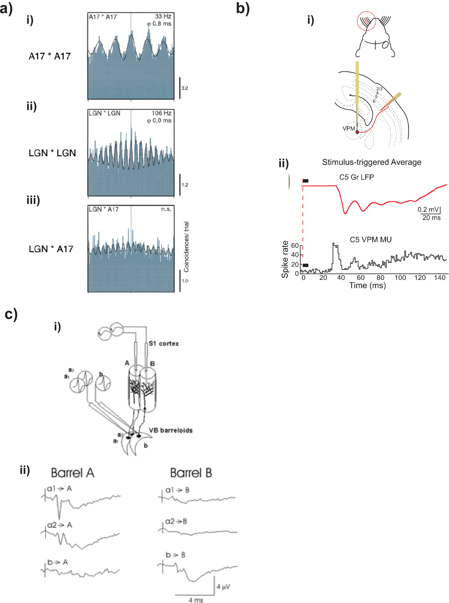
a, Local activity in cat visual cortex. Top: moving stimuli generate coherent gamma oscillations in cat visual area 17. Middle: the same stimuli generate higher frequency oscillations in lateral geniculate nucleus (LGN). Bottom: visual cortex and LGN oscillations are not coherent with each other (n.s., not significant). Adapted with permission from Castelo-Branco et al.¹⁴⁷, Society for Neuroscience. b, Gamma oscillations in developing rodent cortex due to thalamic input. Top: experimental setup for simultaneous recordings of single-whisker evoked responses in the thalamic ventroposterior medial nucleus (VPM) whisker C5 barreloid and corresponding cortical barrel column in the postnatal day 6 rat. Bottom: responses averaged across 100 whisker deflections in the matching barreloid of VPM thalamus, showing multiunit (MU) poststimulus time histogram (black) in the VPM and evoked LFP (red) in the granular layer of the corresponding cortical barrel. Cortical LFP gamma activity is present at a stage of development during which cortical circuits do not generate gamma activity. Thalamic multiunit activity preceding cortical gamma implies that cortical LFP is due to incoming thalamic spiking and not local cortical spiking. Adapted with permission from Minlebaev et al.¹⁴⁸, AAAS. c, LFP activity in rabbit cortex due to thalamic input. Top: experimental setup. Two thalamic electrodes recorded from neurons in neighboring ventrobasal (VB) barreloids (labeled a and b) and cortical electrodes recorded spike-triggered averages in the topographically aligned (and neighboring) primary somatosensory cortex (S1) barrels (labeled A and B). Spike-triggered averages were generated by two neurons in barreloid a (a1 and a2) and by one neuron in barreloid b. Bottom: spike-triggered averages elicited in barrel A by barreloid neurons a1, a2, and b are shown at left. Spike-triggered averages elicited in barrel B by the same three VB neurons is shown at right. Reproduced with permission from Swadlow and Gusev¹⁴⁹, The American Physiological Society.

Modeling

All extracellular potentials stem from summed contributions of transmembrane currents across the surfaces of neurons (and in principle also glia cells; see Box 1)^4,5,10. In this sense, the biophysical forward model of field potential recordings is similar to that of spike recordings. However, field potentials differ from single-neuron recordings in important ways. Single-neuron spike recordings have a single source—a neuron that generates action potentials at discrete events in time. The single-unit measurement is a classification: we want to determine whether the neuron has generated an action potential. Distant sources can only contribute to the noise floor above which single-neuron activity must be discriminated. In contrast, field potentials are continuous signals that do not have a single source⁵. A field potential measurement has contributions from different sources weighted according to the measurement modality—LFP, ECoG, EEG or MEG. Of the various potential sources, the largest cellular contribution comes from neurons that generate the largest current dipoles, those with extended, oriented dendritic arbors (see Fig. 2a). Temporally correlated synaptic inputs at restricted dendritic sites also contribute strongly to field potentials. Distant sources can contribute directly to field potentials owing to volume conduction or, for MEG, field spread. Volume conduction occurs because electromagnetic fields propagate through biological tissues^6,11. Consequently, field potentials reflect the organization of large-scale brain dynamics.

Fig. 2 |. Forward models.

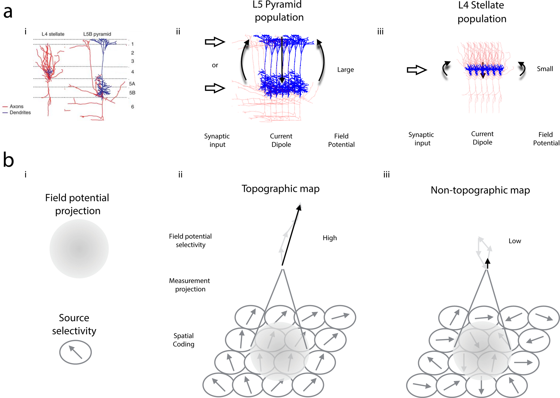
a, The biophysical forward model predicts that the amplitude of field potentials generated by populations of neurons will depend on the dendritic morphology of local neurons, as well as the somato-dendritic location of the incoming synaptic inputs, and will not depend on the axonal morphology of local neurons. Box 1 discusses other contributions. Left: layer (L) 4 stellate neurons have restricted and symmetric dendritic arbors (blue) with extended axonal distributions that ramify locally (red). L5 pyramidal neurons have the most extended dendritic arbors and relatively sparse axonal distributions. Image adapted with permission from Shepherd et al.¹³⁸, Springer Nature. Synaptic input to a population of neurons generates a current dipole that gives rise to the extracellular field potential signal according to the biophysical forward model. Center: populations of L5 pyramidal neurons can receive synaptic input to the apical or basal dendrites and generate large-amplitude field potentials in each case. Right: populations of L4 stellate neurons can receive synaptic input near the cell body and generate relatively small amplitude field potentials. Note that this is a simplification. The size of the generated potentials will depend on how displaced the return currents are from the synaptic input currents and spatial distribution of the return currents. The return currents depend on several other factors, including the thickness and branching of the dendrites. For example, in some cases about half of the current injected into the apical dendrite of a L5 neuron will return through the soma, and even less in neurons with a thinner apical dendrite¹³⁹. Density and strength of synaptic inputs, membrane potential, and membrane conductance of the postsynaptic population will also contribute to the magnitude of the generated potentials¹⁴⁰. b, Functional variant of the biophysical forward model. The functional variant predicts that information can be decoded from field potentials depending on the measurement projection given by the biophysical forward model and the spatiotemporal distribution of source selectivity in the brain. Left: the measurement projection underlying a field potential recording pools information across a volume (shaded). Spatial aspects are illustrated here, but note that the measurement projection also depends on temporal correlations (see Box 1). The selectivity of the underlying neuronal sources can be expressed as a directional arrow. Center: field potentials will exhibit strong selectivity if the spatial distribution of the underlying source selectivity is organized so that the measurement projection pools one or several sources with similar selectivity. Right: field potentials will exhibit weak or no selectivity if the spatial distribution of the underlying source selectivity is disordered and if the measurement projection pools several or many sources. Note that even if the spatial distribution of the underlying source selectivity is organized, weak selectivity can arise if the measurement projection pools over a much larger spatial extent.

While biophysical forward-modeling schemes for field potential signals are well established^6,10,12, several issues remain controversial. One controversy concerns the frequency dependence of the electrical conductivity of the extracellular space; i.e., whether volume conduction biases LFP and EEG recordings toward certain frequencies¹³. Field potential power has been observed to decay in power law-like way (1/f^a) for higher frequencies. Establishing a power law is challenging because the range of frequencies is limited, typically only spanning two or three orders of magnitude. While the reason for any power law remains unclear, potential explanations include scale-free dynamics, the capacitive effects of neuronal membranes, and noise from evenly distributed ion channels across dendrites^14–16. Early experiments found very little frequency dependence in the frequency range of interest for neuronal recordings^17,18, implying that the extracellular medium is essentially resistive—i.e., ohmic with a negligible capacitive component. Subsequent observations showed a strongly reduced electrical conductivity for frequencies below 100 Hz¹⁹ suggesting a strong low-pass filtering of the LFP and EEG from the extracellular medium²⁰. A series of further studies, however, using a variety of measurement setups, have confirmed the early findings and found only weak frequency dependencies^12–25. Thus, on balance the experimental observations seem to point to a largely resistive extracellular medium.

The contribution of spiking events to field potentials is somewhat controversial. In cortex and hippocampus, the high-frequency part of the extracellular potential—i.e., above some hundred hertz—is thought to be dominated by spiking activity. Likewise, the low-frequency part—i.e., below some tens of hertz—is thought to be dominated by the subthreshold extracellular signatures of synaptic activation^4,5, although spikes also contribute²⁶. Spikes are far more likely to contribute to intracortical microelectrode LFPs than to the EEG recorded from a scalp electrode. The crossover frequency—i.e., the frequency above which the spike contributions start to dominate—depends on the competition between subthreshold and spiking signal contributions. The result depends on brain area and brain state: in hippocampus, spikes contribute to the extracellular signal for frequencies down to 100 Hz^27,28; in monkey visual cortex, extracellular signal frequencies as low as ~50 Hz have been associated with spiking²⁹. In general, the contribution of spiking events depends on the shape and amplitude of the action potential waveform and the firing rate³⁰.

Inverse modeling to infer neuronal sources also presents controversies. Inferring neuronal sources from MEG or EEG is called source reconstruction. Direct validation has been performed with electrical stimulation of an implanted electrode^31,32, and expected results have been obtained, for example, in the case of activity in early sensory cortices^33–35 and in the case of dipole sources for epileps³⁶. However, in general, more information is always required in addition to the recorded potentials or fields; sources may be distributed with many dipoles and/or higher order multipoles, and reconstruction depends on information that is often unavailable^37,38. Inferring neuronal sources from LFPs has typically involved current source density (CSD) analysis. Direct empirical validation of CSD analysis has also proven challenging³⁷. Although the assumption of charge conservation is well established, it can be difficult in practice to determine exactly where the currents flow.

Finally, the ability to read out, or decode, information processing from the brain underlies the development of brain-machine interfaces and neural prostheses and depends on the choice of neuronal signal (spiking, LFP, ECoG, EEG, MEG). Field potential decoding analyses depend on how field potentials measure selectivity of the underlying neuronal sources, as well as the spatiotemporal organization of the source selectivity. We can summarize these factors in a functional variant of the biophysical forward model. The functional forward model describes how neuronal activity varies as result of different task conditions and how this generates selective field potential responses (Fig. 2b). This model involves the biophysical model, along with how populations of neurons encode behavioral or task-relevant variables. The functional forward model predicts that field potentials are more selective for field potential modalities in which the measurement projection is spatially confined, at sites where the weighted sources encode similar variables, and for task variables that change the spatial-temporal activity correlations to which field potentials are sensitive.

Relatively little work has investigated field potential selectivity in terms of the forward model, and the nature of field potential selectivity remains controversial. An early view was that LFP selectivity differed from spiking recordings and was similar to EEG selectivity. However, empirical studies show LFPs contain more sensory and movement information than EEG and are more comparable to the information available in the spiking activity of single neurons^39–45. Information about reach, grasp and speech actions are also present in human ECoG recordings^46,47. While more work is needed, in cortex, the presence of field potential selectivity comparable to single neuron selectivity may reflect the underlying columnar organization of cortex^39,41,44,45. Since field potential recordings are easier to obtain than recordings of spiking activity, these and other studies suggest that ECoG and/or LFP signals, in addition to spiking, may serve as a basis for a high-performance brain-machine interface⁴⁸. For MEG and EEG, multivariate classification approaches also reveal neuronal encoding of various forms of sensory and cognitive information^49–52. MEG and EEG selectivity is also shaped by volume conduction in a process called spatial filtering^6,53. If many sources with different dynamics occur in dipole layers of different sizes, the measured MEG and EEG signal is dominated by the temporal dynamics of those source components that are synchronized more broadly over the cortical surface^5,37. Consistent with these observations, MEG and EEG signals appear to be less selective than ECoG signals, which in turn appear to be less selective than LFP signals^39,54,55.

Analyses and interpretations

Field potential recordings are time series—a series of measurements ordered in time—that reflect neuronal dynamics. As a result time series analysis tools that measure dynamics, such as spectral analysis⁵⁶, are often used to characterize field potentials^57,58. The first three sections present time series analysis and interpretations that depend on the biophysical forward model. In “Activation,” we discuss how to assess the signal characteristics at a given site and their changes with experimental conditions. In “Correlations,” we discuss how to characterize correlations in activity between sites. In “Communication,” we detail tests for directed influences that may reflect neuronal communication. The fourth section, “Coding,” considers the functional aspects of the forward model. We discuss neuronal coding and how information in the underlying neuronal activity can be decoded from field potentials. In each section, we discuss the associated analyses and interpretations.

Activation.

We first focus on estimating the magnitude of the activity and testing for differences, before turning to interpreting spectral features and oscillations.

Statistical estimation.

Two classic measures of time series are the autocorrelation or autocovariance and the power spectral density function, which we will refer to as the spectrum (Fig. 3). The autocorrelation measures how much activity is correlated at two points separated in time, τ = t₂ - t₁, also called lag. The spectrum measures how much power the activity contains at each frequency f The spectrum and autocorrelation function provide complementary information but are not equivalent measures of activity. The spectrum reveals spectral peaks (that may correspond to physical sources) that can be difficult to distinguish in the autocorrelation function. Conversely, the autocorrelation function reveals how rapidly a signal tends to become uncorrelated over time, which is not directly evident from the spectrum itself.

Fig. 3 |. Time series and spectral estimation.

a, Left: the sampling rate of a time series, F_s, is inversely related to the sampling interval, df. The maximum frequency that can be resolved in a time series, called the Nyquist frequency, is determined by the sampling interval and equals F_s/2. The bandwidth W is the lowest frequency that can be resolved in a time series, also called the Rayleigh resolution. It is inversely related to the duration of the observation window and equals 1/T. Right: time-frequency plane. The Rayleigh resolution is an example of the time-frequency uncertainty principle, which states that the product of the resolution in time, T, and resolution in frequency, 2W, must be equal or greater than 1; i.e., 2 WT ≥ 1. We can increase the time × bandwidth product by increasing the analysis interval T, and hence smoothing more in time, or by increasing bandwidth W, and hence smoothing more in frequency. In each case, we effectively assume that the properties of neuronal activity are constant within the chosen time and frequency resolution that leads to a smoother, less variable estimate. Image reproduced with permission from Pesaran (2008)⁵⁷, copyright 2008, Society for Neuroscience. b, Spectrum of LFP activity in macaque posterior parietal cortex. Left, single-trial, 500-ms periodogram spectrum estimate. Right, single-trial, 500-ms, 10-Hz multitaper spectrum estimate. Image reproduced with permission from Pesaran (2008)⁵⁷, copyright 2008, Society for Neuroscience. c, Spectrogram of LFP activity in macaque posterior parietal cortex averaged across nine trials. Each trial is aligned to the presentation of a spatial cue, which occurs at 0 s. Saccade and reach are made at around 1.2 s. Left: multitaper estimate with duration of 500 ms and bandwidth of 10 Hz. Right: multitaper estimate with duration of 200 ms and bandwidth 25 Hz. White rectangle shows the time-frequency resolution of each spectrogram. The color bar shows the spectral power on a log scale in arbitrary units. Image reproduced with permission from Pesaran (2008)⁵⁷, copyright 2008, Society for Neuroscience.

Spectrum and correlation function estimates assume that neuronal activity is stationary. Stationarity means the signal statistics, power and correlations remain constant over time. Strictly speaking, stationarity is never satisfied. Nonstationarities occur with transient events. The most extreme example is the nonstationarity of activity around the time of stimulus onset. However, even in the absence of changes in sensory input, brain activity displays transient events that can wax and wane, such as beta activity in the frontal cortices and ripples in the hippocampus. Nonstationarities can also occur across different time scales, such as fluctuations in high-frequency synchronization following low-frequency excitability changes⁵⁹, and can occur when activity appears stationary—for example, sustained stimulus-induced gamma oscillations in visual cortex or sustained theta oscillations in rodent hippocampus during walking. Changes also occur spontaneously—for example, as one spontaneously drifts back and forth from an aroused to an unaroused state^60,61. In each case, the spectrum and autocorrelation averaged across these fluctuations will not be a good descriptor of the data.

If the changes occur relatively slowly or the changes can be detected, we can select or detect periods in which the signal is locally stationary. We can then compute the spectrum for these periods. Appropriately selecting time periods depends on understanding a fundamental time-frequency uncertainty relationship: the product of the time resolution of the spectral estimate, T, and the frequency resolution of the estimate, W, is always greater than 1 (Fig. 3a). With a time window of duration T, the lowest resolvable frequency is 1/T. Deciding how to trade off time and frequency resolution is complex, as there may be no single best answer. Resolving signals at low frequencies, such as below 10 Hz, requires frequency resolution on the order of 1 Hz. Time resolution is, at best, 1 s. Conversely, resolving signals that change during behavior requires time resolution of, say, 200 ms. Frequency resolution is then 5 Hz or more. Many spectral estimators are available, each with different statistical properties of bias and variance that vary with the desired time-frequency resolution (Fig.3b,c). The Supplementary Note discusses spectral estimation with guidelines for best practices.

Interpreting spectral power.

In general, field potential power decays in a power-law-like way (1/f^a), especially for higher frequencies. The 1/f shape of the spectrum can generally be sensitive to the overall firing rate of the underlying population or the number of active neurons, with linear offsets in power resulting from an overall change in the firing rate¹⁵. Neuronal spike waveforms can also appear in the LFP, especially if the amplitude of spike waveforms in an LFP recording is large. The LFP spectrum at frequencies above 50 Hz can be especially sensitive to changes in firing rate³⁰. LFP power is highly sensitive to the synchrony of the underlying local and afferent-remote populations, so the overall shape of the spectrum may reflect a heterogeneous mixture of temporally structured signals that spanning a range of frequencies. The steepness of the 1/f^a curve can also change as a result of changes in the membrane time constant. Membrane time constants can depend on the overall level of activation in the circuit⁶², as well as on the activation of NMDA receptors because these have much slower excitatory postsynaptic potentials than AMPA receptors^15,63. Another contributing factor is noise. Activity at high and very low frequencies often has poor signal-to-noise ratio—for example, EMG noise (high frequencies) or electrode or cable movement (low frequencies) may attenuate observed changes in the underlying signal.

Interpreting oscillations.

In addition to the 1/f trend, transient, phasic changes in spectral power can be observed to come and go. Detecting a candidate ‘oscillatory’ event depends on setting a threshold. Interpreting these events as changes in a neuronal source is of great importance. In particular, observations of spectral peaks in activity at particular frequencies are often referred to as oscillations. Oscillations are often depicted in the theoretical literature as narrow-band, periodic, sometimes even sinusoidal phenomena. However, theoretical oscillators, like a pendulum, generate features at particular frequencies and do not contain multicomponent or broadband features. In comparison, physiological neuronal ‘oscillations’ often have a clear broadband or band-limited character^64,65 and change quickly^66,67.

This caveat notwithstanding, we often want to know whether an increase in spectral power indicates an increase in the number of active neurons or an increase in temporally structured or synchronized neuronal activity. The absence of a spectral peak does not necessarily mean that there is no synchronized activity in the underlying neuronal activity. If there is an underlying oscillatory pattern, a peak in the spike-field coherence (SFC) may be present even without any peak in the LFP spectrum⁶⁸. Thus, if spiking is coherent with a field potential, temporally structured spiking exists and a local source contributes to the field potential^39,69, and this source may be said to reflect oscillatory activity. The Supplementary Note presents measures that go beyond second-order correlations to capture correlations between different frequencies and phase-amplitude coupling.

Interpreting cellular sources.

Interpreting field potential recordings in terms of cellular sources is limited by the ill-posed nature of the inverse model. Clear interpretations are sometimes available when a local neuronal population generates the currents measured by field potential recordings, such as for the hippocampal theta rhythm⁷⁰. Defining local current generators is called current-source density (CSD) analysis. According to Maxwell’s equations and Ohm’s law for the extracellular medium, the local current generators are given by a second spatial derivative of the LFP signals in all three directions, called the Laplacian⁶. Therefore, CSD analysis requires invasive recordings with electrode arrays with high contact density, typically 50–200 μm intercontact spacing or less (Fig.4a)^2,5,71. CSD analysis yields the net volume current density that enters (source) or leaves (sink) the extracellular medium through cell membranes (Fig. 4b). Consequently, CSD analysis is a more local measure than the LFP and is easier to interpret in terms of neuronal activity.

Fig. 4 |. Current source density analysis.

a, A cylindrical model in infinite medium, showing the relationship between current source density (CSD), current flow and field potential for the simple case of a columnar geometry receiving input at a particular layer. The geometry is a cylinder having a diameter-to-length ratio of 0.5 and embedded within an infinite medium of finite conductivity. Because there is circular symmetry, only the points on the z axis along the cylinder are shown. The CSD (transmembrane current l_m; left) gives rise to a current flow (J_z; center). Current flow establishes the field potentials (V_z; right). Current density enters the cylinder and returns below. This generates a downward current flow above and below the source and sink and an upward current flow between the source and sink. The resulting field potentials extend beyond the generating current source. Thus, CSD has higher spatial resolution than field potentials. Adapted with permission from Nicholson and Freeman², The American Physiological Society. b, Laminar patterns of auditory responses in the auditory cortex. Line plots show the LFP responses recorded using a linear array multielectrode with 100-μm intercontact spacing (schematic on left). Color plot (center) shows the corresponding laminar LFP profile, with negative deflections in red and positive deflections in blue. CSD profile (right) is estimated using the second spatial derivative of the field potential profile. Red depicts extracellular current sinks associated with net local inward transmembrane current flow. Blue depicts extracellular current sources associated with net local outward transmembrane current flow. Selected multiunit activity (MUA) responses are superimposed on the CSD plot. Vertical thin lines indicate stimulus onset. Here, the peak of multiunit activity corresponds to the peak negativity of the LFP and the current sink (CSD) at the response onset in layer 4. Asterisk indicates a superficial sink that produced the N50 feature in the LFP measured in superficial sites. Image adapted with permission from Kajikawa and Schroeder¹⁴¹, Elsevier. c, Limitations of traditional CSD estimation method. Simulated one-dimensional recordings for simplified CSD profile in a. Estimated (est.) CSDs for increasing diameter-to-height ratios, as indicated by the number and inset in the lower left of each panel. Diameter refers to the diameter of the source. All estimates are based on the second spatial derivative formula of the traditional CSD method. Arbitrary units, negative values to the left and positive to the right. Spurious sources and sinks are inferred for small diameter activity. Estimation error stems from the incorrect assumption of an infinite activity diameter perpendicular to the laminar electrode. To avoid spurious source and sink inferences, a full three-dimensional CSD analysis is needed. Such an analysis can be achieved by making measurements of field potentials in all three spatial directions¹⁴² and using second spatial derivative methods. Alternatively, spurious source and sink inferences can also be avoided by using prior constraints or assumptions as is done in the iCSD¹⁴³ and kCSD¹⁴⁴ methods. Image reproduced with permission from Pettersen et al.¹⁴⁵, Cambridge University Press.

Traditional CSD analysis assumes that there is no variation of the neuronal activity in the horizontal directions. Thus, CSD is given by the double spatial derivative in the depth direction. This approximation can be problematic as, in primary sensory systems, inputs to cortex can be quite focal and significant tangential currents can exist as a result of tissue curvature (Fig. 4c), but new CSD estimation methods can account for this. Traditional CSD analysis also assumes that the electrodes adequately sample the currents within the volume. Ideally, three-dimensional sampling of the volume would be preferred to reduce CSD estimation error using the second spatial derivative method⁶. In general, interpreting current sources in terms of cellular sources, such as whether a sink or source is active (for example, due to synaptic current) or passive (a return current), depends on additional information about the anatomical connectivity of presynaptic input-generating populations and geometry of postsynaptic populations. Box 2 and the Supplementary Note present a more detailed discussion.

Correlation.

Networks of neurons generate brain dynamics, and correlated patterns of activity are ubiquitous. There are many ways to capture dependencies between neuronal signals. Here, we will focus on linear measures of coupling, correlations that are well understood in statistical terms and are in widespread use.

Correlation and coherency.

The cross-correlation function measures correlation in the time domain. In the frequency domain, we can use the spectral coherence function, which is defined as the cross-spectrum between signals normalized by the spectrum of each signal. Coherency is the correlation coefficient that measures the strength of linear association as a complex-valued regression coefficient. The magnitude of the coherence is proportional to the strength of linear association. The phase of the coherence reflects the relative timing but not necessarily a time delay (see Supplementary Note).

Like the spectrum and the autocorrelation function, the coherency and the cross-correlation function offer complementary information. An important advantage of the coherency is that it is normalized by power at each frequency. The cross-correlation function is normalized by total variance of each signal, which is the integrated power over all frequencies. As a result, the coherency can often detect frequency-localized effects better than the cross-correlation function can. The latter is typically dominated by frequencies with more signal power, which are often at lower frequencies.

Estimating coherency depends on similar factors as estimating the spectrum. In general, coherence estimates typically require more degrees of freedom than spectrum estimates. In effect, coherence measures the correlation present in a scatterplot of points, where there is one point for each pair of degrees of freedom. Unlike the spectrum, the distribution of spectral estimators for the coherence is, in general, complicated and depends on the strength of coherence. Several strategies exist to address these issues, and statistical tests should be based on appropriate permutation tests^72,73.

Two processes that do not interact can appear to be coherent by virtue of being nonstationary⁷⁴. Estimating coherency and cross-correlation in locally stationary time intervals to give time-varying coherence spectra, called coherograms, is therefore critical. Since coherence estimates with few degrees of freedom are positively biased, particular care should be taken when interpreting coherence over short time periods using few degrees of freedom.

Spike-field coherence.

Whenever possible, interpreting field potentials in terms of cellular sources is best done directly, using simultaneous measurements of spiking activity. The spectral analysis of spike-field relations largely matches that of field potentials. This is because point processes admit a spectral representation like that of other time series. As a result, SFC is an important tool for understanding the relationships between LFPs and underlying spiking activity⁵⁸. SFC is the correlation coefficient of a regression, analogous to the coherence between two field potentials⁷⁵, that quantifies how predictable LFP activity is as a linear function of the spike times. SFC specifically measures how neurons tend to fire spikes at particular phases of LFP activity. The spike-triggered LFP measures spike-field relationships in the time domain and is useful for resolving time delays between spiking and events in the LFP. Statistical considerations mean that the SFC is preferred over the spike-triggered average (see Supplementary Note).

SFC sensitively reveals the locking of neurons to synchronized synaptic inputs, which also lead to postsynaptic currents and thereby the LFP signal. The broad-band properties of the LFP spectrum itself may mask spectral peaks. However, if there is an underlying oscillatory pattern, a peak in the SFC may be present even without any peak in the LFP spectrum^76–78.

Contamination of the LFP by action potentials is a major concern when analyzing phase correlations and SFC. Attenuation of neuronal spike contamination in LFPs can be attempted by removing spikes from the LFP signal⁷⁹. However, residual spike contamination effects may remain. In general, best practice is to use spike and LFP recordings from different electrodes separated by several hundred micrometers.

Signal-to-noise ratio confound.

A critical issue when interpreting correlation and coherence is that both measures are influenced by the relative weight of neuronal signals (signal components) versus other signals (noise components). This leads to an important confound: a change in the signal-to-noise ratio (SNR) will change the measured correlations without a change in the underlying neuronal interaction or functional connectivity. If signal components are more correlated than noise components—for example, because of a specific interaction between neuronal populations of interest—an increase in signal amplitude or a decrease of noise amplitude can also increase observed correlations. If noise components are more correlated than signal components—for example, because of field spread from remote neuronal sources to two signals—an increase in noise or a decrease in signal amplitude can increase observed correlations. Correspondingly, changes in noise can also lead to decreases in observed correlations without changes in the underlying neuronal interaction. The Supplementary Note illustrates these effects mathematically.

One strategy to limit concern is to check for changes in signal amplitude that may reflect a potential change in SNR and to only focus on changes in dependencies between signals that either are not paralleled by changes in signal amplitude⁸⁰ or cannot otherwise be accounted for by changes of SNR. Another strategy is to stratify the activity by amplitude. Similarly, the power or SNR of the signal of interest can be binned and correlations can be computed within each bin.

SNR confounds also affect the interpretation of SFC. Enhanced spike-LFP coupling when LFP power increases could reflect greater contribution of spike-locked neuronal sources to the LFP instead of stronger spike-locking of these sources. Differences in mean spiking rates across conditions can also affect the corresponding SFC estimates without requiring true changes in functional connectivity⁸⁰. To mitigate these effects on SFC, spike trains can be decimated to equalize the mean rates across conditions. This involves randomly deleting spike events to match the total number of spikes across conditions. Spike events that are deleted randomly will not alter the underlying spike-field coupling⁸¹. A complementary parametric approach to SFC based on point process, generalized linear models (GLMs)⁸² can also be used to separate the contribution of changes in firing rates and changes in phase coupling to LFP oscillations when assessing spike-field relationships across different tasks or conditions^83,84. Finally, SFC quantification based on the pairwise phase consistency (PPC) metric avoids spike rate and spike count biases⁸⁵. With this approach, the synchronization between spikes and LFP is determined by first estimating the LFP phase at the time of each individual spike and then quantifying the similarity of pairs of spike phases.

Volume conduction.

Coherence is particularly sensitive to volume conduction and common modes due to distant sources. Volume conduction is of particular concern in the rodent brain. In the rodent, theta and beta frequency range potentials generated by the hippocampal formation can be measured across the neocortical and subcortical neuropil, which makes it difficult to perform valid coherence analysis between brain areas^86,87.

One effective strategy assumes a forward model in which the impedance of brain tissue is resistive and not capacitive²¹. Field spread due to volume conduction is then effectively instantaneous and does not alter the imaginary component of the cross-spectral density. This yields several measures such as the imaginary part of coherenc⁸⁸, phase lag index (PLI)⁸⁹ and weighted phase lag index (WPLI)⁹⁰ (see Supplementary Note). Best practice is to analyze activity at each site to assess the presence of volume conduction before interpreting the correlated activity patterns.

Correlations due to volume conduction can survive source reconstruction^91,92 and rereferencing procedures. The widely used common-average reference averages all recorded signals and thereby introduces artifacts to which correlations are particularly sensitive. While careful selection of a reference electrode can help suppress shared signals (see Supplementary Note), care should be taken to assess whether the rereferencing actually removes the common reference. We can also perform spatial filtering to suppress volume conduction by making use of a bipolar reference, computing the CSD or Laplacian and applying source reconstruction or beam-forming techniques described above. The CSD or Laplacian method removes very large-scale, regional or global coherence, as well as volume conduction.

Communication.

Given evidence of correlations between two sites in a network, X and Y, we can ask whether the correlations reflect putatively causal interactions with a particular directionality: for example, X drives Y, or X → Y. Many causal inference procedures exist. Here, we focus on the analysis of Granger causality (GC) because it is relatively simple and well understood, derives from spectral analysis and is in widespread use.

We should first make clear that, in general, no statistical procedure can accurately recover causal influences if unobserved nodes in the network, or hidden nodes, generate the main interaction effects. This is true for spiking and field potential recordings. Consider a three-node network with common input: if X → Y and X → Z with a longer delay, unless X is measured, statistical inferences will likely report Y → Z. Consider another network X → Y → Z. In this case, unless Y is measured, the influence may be incorrectly estimated as X → Z. Field potentials reflect subthreshold currents, but the transfer of those currents to spike output can vary from case to case, complicating causal inferences. Thus, an influence of field potentials recorded in X on field potentials recorded in Y suggests that spike output of neurons in X influences current flows in neurons in Y because only spikes travel from X to Y; yet this does not necessarily mean that spike output in Y is influenced. Box 2 analyzes this topic.

Statistical estimation.

Since estimating time delays from correlation or coherence functions can be confounded, additional measures are needed to infer causality and directed influences. Measures based on GC^93,94 assess the direction of influence or causality in terms of temporal prediction among stochastic processes (Fig. 5). Informally stated, a stochastic process X is said to ‘Granger-cause’ or drive a stochastic process Y if the history of X adds to the prediction of Y beyond what can be predicted based only on the history of Y itsel^95,96. GC can be statistically assessed in terms of likelihood ratio tests^97,98 and can be computed in both the time and frequency domains. In addition, if multiple neuronal groups have been recorded simultaneously, the conditional GC can distinguish (i) between direct versus indirect interactions—i.e., X → Z vs. X → Y → Z, corresponding, for example, to mono- vs. polysynaptic interactions—or (ii) between common inputs with different delays vs. direct interaction—i.e., between X → Y and X → Z with a longer delay vs. the direct interaction Y → Z. Software packages to compute GC measures are publicly available⁹⁸.

Fig. 5 |. Granger-causal inferences.

a, Schema of multivariate autoregressive models. Each time series is modeled as a linear combination of its own past, the past of the other time series, and an innovation term. These signals are corrupted by measurement noise that can be either correlated or uncorrelated. b, Cross-correlation function example, showing that cross-correlation methods are not appropriate for detecting causal relationships. In this case, the cross-correlation function tells us that future (lagging) but not past (leading) values of y(t) are strongly correlated with x(t). Despite this, the Granger-causal influence from y(t) to x(t) is stronger than the influence from x(t) to y(t). c, Application of reversed GC testing to LFP data from monkey primary visual cortex (V1) and V4. Interaction in the gamma band shows full reversal with time series reversal and is therefore robust. This behavior is shown across V1-V4 pairs. In the beta range, GC causality does not reverse with time series reversal, indicating a potential influence of correlated noise.

Since GC measures typically depend on parametric models, model mismatch is a concern⁹⁹. While GC measures using nonparametric spectral estimates have been proposed¹⁰⁰, a parametric model derived from the nonparametric estimates is still needed. Nonparametric estimates are preferred because they have improved bias and variance properties compared with parametric estimates (see Supplementary Note). The GC influence measure is also subject to a SNR concern because the GC influence assumes there is no measurement noise (see Supplementary Note). GC estimates also tend to be strongly positively biased by sample size, and re-estimating the GC after shuffling the time series may be needed to control for sample size bias.

Like other spectral analyses, GC analyses can be extended to address slow nonstationarity by using a moving window. Causal inferences depend on model fitting, and nonstationarity can lead to model fitting and interpretation problems for causal inferences. For example, the evoked or event-related potential averaged across trials is subtracted from each trial to ensure stationarity or, assuming a linear additive model, to separate the signal from ongoing background activity. However, if slow across-trial nonstationarities are present as a result of changes in neuronal excitability, attention or fatigue, the evoked response can show trial-to-trial changes in amplitude, latency and waveform (see Supplementary Note). This nonstationarity will affect the interpretation of GC, as well as other spectral measures such as power and coherence^101–105. Amplitude changes can be effectively suppressed by fitting the evoked response per trial^101,106. Latency and waveform changes are more complicated to model, and removal of trial-to-trial variability due to these changes should be performed with caution.

Causal inferences ultimately require empirical validation using interventions. This said, inferences based on interventions also require caution. Interventions often shift the system out of the normal physiological range. Since the intended and achieved manipulations can differ, interventions can also lack validity. Electrical microstimulation preferentially stimulates axons, not cell bodies¹⁰⁷. Optogenetic stimulation affects illuminated neurons simultaneously, potentially changing phase delays across layers¹⁰⁸. In general, experiments should use small perturbations to avoid driving the system out of range. Experimental designs should also parametrically vary manipulation conditions, instead of simply comparing manipulation and no-manipulation conditions, to more directly infer the underlying causal mechanisms.

Coding.

Understanding nervous system function depends on the functional forward model—how information is present in activity, what form it takes, and whether and how it can support behavior. Coding implies the presence of correlations between a neuronal signal and external events, such as stimulus onset, and internal events, such as the spike of a neuron or the phase of another neuronal signal. Neural decoding quantifies the information present in those correlations.

Information about the task-relevant variables can be decoded from field potential amplitude¹⁰⁹, power^39,42, coherency magnitude¹¹⁰ and phase⁷⁷, and phase-amplitude coupling¹¹¹. Information can also be decoded using the phase relations between spikes and the surrounding LFP, SFC, as well as by using GLMs that relate spiking probability to the amplitude and phase of LFP oscillations⁸⁴. In the hippocampus, the SFC is strong in the theta range, and its phase carries information about the position of the animal¹¹². Phase relations between LFPs carry similar information (Fig. 6a)¹¹³. During short-term memory, SFC in the beta band (~30 Hz) underlies phase-dependent coding of short-term memory information in prefrontal cortex¹¹⁴. Different memory items are preferentially encoded at different 30-Hz phases (Fig. 6b). Posterior parietal and frontal neurons that display coherent phase relations, termed coherent neurons, encode information about behaviorally relevant processes such as decision making and coordination more accurately than neurons that do not fire spikes coherently^69,115,116. Information about movement choice is also modulated by LFP phase¹¹⁷ (Fig. 6c). In visual cortex during visual stimulation, SFC is strong in the gamma band, and its phase depends systematically on stimulus orientation¹¹⁸. Spikes occur earlier in the gamma cycle for stimuli close to the preferred orientation of the spiking neuron than for nonpreferred stimuli (Fig. 6d). In general, phase relations in the gamma frequency band are diverse and change with stimulation and also, for example, with selective attention⁷⁷.

Fig. 6 |. Phase-dependent neuronal coding.

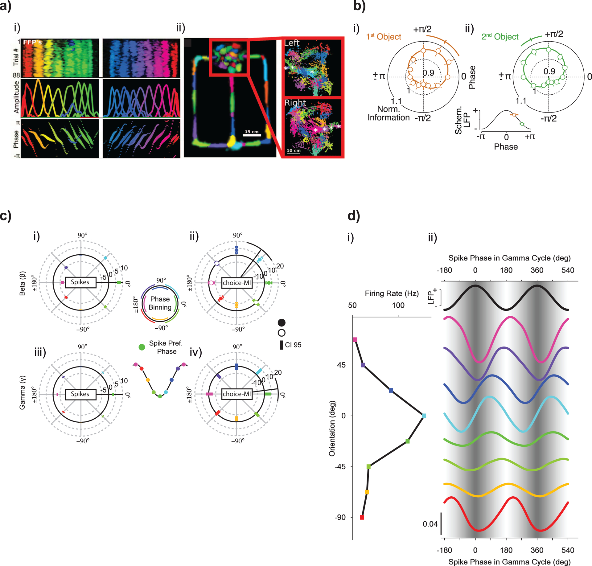
a, Place information encoded by the phase of hippocampal LFP activity. Left panels: feature-tuned field potentials (FFPs) recorded from the hippocampus during running on a linear track (top). FFPs uniformly tile the length of a linear track. The spatial extent and spacing of different FFPs is largely homogeneous across the track (middle). FFPs exhibit phase precession with respect to the first principal component of LFP activity (bottom). Place-field hues are assigned based on location of maximal activation. Right panels: activation of FFPs during running in a T-maze. Waiting area is enclosed in a red box. Far right shows close-up of activations in waiting area, separated by direction of entry. Asterisks mark activations that are entry-direction selective. Each point represents a time bin where FFP activation exceeded a threshold, its size indicating the magnitude of activation. Hues are assigned to distinguish neighbors. Image reproduced with permission from Agarwal et al.¹¹³, AAAS. b, Object information in PFC spiking during a working memory task depends on LFP phase. PFC neuron spiking encodes the identity of two sequentially presented objects during a delay interval. Spikes carry the most information about the memorized objects at specific phases of the local 32-Hz LFP. Left: optimal encoding of the first presented object is significantly earlier on the falling flank of the 32-Hz cycle. Right: encoding of the second presented object occurs later (permutation test, P = 0.007). Error bars denote s.e.m. Phase dependence induced by stimulus-locked responses was discounted. Image reproduced with permission from Siegel et al.¹¹⁴. c, Choice information in PPC spiking depends on beta and gamma LFP phases. Top left: average phase-dependent histogram of spike count for the beta frequency range. Coloring of the phase bins in all histograms corresponds to the schematic phase binning shown in the center. The spike-preferred phase (dark green) is depicted as a trough in the schematic to capture the tendency of spiking to occur at or near the troughs of LFP activity. The green bin at 0° corresponds to the average spike-preferred phase in the 200–1,000 ms epoch after target onset, when the choice can be made. The radial distance for each phase bin indicates the difference in spike count from random phases. Error bars depict 95% confidence intervals. The radial black line depicts the trigonometric moment of the histogram, with its 95% confidence interval indicated at the end of the line. Top right: as before but for mutual information about choice (choice-MI). Same data as before at each phase bin. Fully colored circles indicate choice-MI significantly different from the average choice-MI across all phase bins (permutation test, P < 0.05). Bottom row: as in the top row but for the gamma frequency range. Image reproduced with permission from Hawellek et al.¹¹⁷. d, Orientation information in V1 spiking depends on gamma LFP phases. Match between stimulus orientation and neuronal orientation preference determines spike phase in the gamma cycle. Data from one example V1 neuron. Left: firing rate as a function of stimulus orientation. Right: the black sine wave at the top and the sinusoidal gray shading in the background illustrate the LFP gamma phase. The colored lines show spike densities as a function of phase in the gamma cycle. The colors correspond to those in the panel at left. All spike density curves are probability densities, normalized such that the mean value of each curve is 1/2 (bottom left calibration bar applies to all curves, and curves are offset along the y axis to correspond to the panel at left). Reproduced with permission from Vinck et al.¹¹⁸, Society for Neuroscience.

Neuronal decoding analyses explicitly test whether our certainty about the value of a random variable is altered by knowledge of another signal. Modern tools for statistical inference, also called machine learning, are increasingly able to detect subtle patterns in large volumes of data^{49,50,52,119,120}. Overfitting can inadvertently occur when parameters and other features in the model, often called hyperparameters or metaparameters, are selected across the dataset¹¹⁹. Cross-validation is the basic technique to address overestimation of decoding performance due to overfitting. Problems arise when the statistical model is very flexible and involves making many decisions during model fitting. Strictly speaking, no part of the data available during any stage of fitting should be used to estimate generalization performance. A good practice in decoding analyses is to divide the data into three subsets: a training set to fit a decoding model, a validation set to compare different choices of hyperparameters or model type, and a test set to assess the decoding performance of the model that has been optimized on the training and validation sets.

Another common issue when estimating neuronal decoding performance is to use features that have been estimated with insufficient statistical degrees of freedom. The resulting estimation noise degrades signal coding. In addition, since single-trial measures contain few degrees of freedom, measures of power, correlation and other aspects of brain dynamics are averaged, typically, across multiple trials. This makes it difficult to measure neuronal coding and how coherence changes trial by trial with, for example, reaction times, attention or choice^115,121,112. One approach is to perform decoding on the relative phase between signals instead, or derive single-trial pseudo-estimates of coherence through jackknifing¹²². The jackknife is more sensitive and accurate than approaches based on sorting and binning of trials¹²³. Another strategy is to use a classification approach and decode activity on groups of trials with similar single trial performance as if they were simultaneously recorded¹¹⁵.

The analysis of neuronal coding in field potentials should not be conflated with the mechanisms by which neurons process information and compute. Field potentials can in some cases influence neuronal information processing owing to ephaptic coupling^124,125. However, analyses to decode field potentials neither imply nor depend on whether ephaptic coupling comprises the underlying mechanism. The ability to decode information from field potentials can have mechanistic implications.

Phase relations in field potentials may reflect levels of neuronal excitability, may carry behaviorally relevant information and may influence neuronal communication. Theoretical studies suggest that the phase-leading neuronal activity exerts a stronger influence over the lagging one than vice versa¹²⁶. Experimentally, the phase-leading recording site shows a transfer entropy to the phase-lagging site¹²⁷. Naturally, care is needed when making causal inferences. Phase precession, whereby the position of the rodent and phase of firing of a place cell correlates with theta LFP activity, is an important link between population coding and oscillatory dynamics. However, information in spiking about spatial position according to theta phase does not necessarily mean the signal has a causal or mechanistic role in the underlying computation. Coding may simply reflect correlation with a latent cause. This concern is a general one, and it also applies to inferring a mechanistic role for coding by single neurons where none may be present^128,129.

Conclusion

We have discussed strategies for analyzing and interpreting a range of field potential recording modalities spanning microns to centimeters. The forward model is the central construction. Biophysics, geometry and anatomical connectivity of neuronal populations are the principal ingredients. Several obstacles hinder future progress. One important direction is to simulate virtual experiments using computational models. In these experiments, the ‘ground truth’ is known and the measurement projection from activity space can be defined. Data from virtual experiments can generate model-based benchmarking data. Such benchmarks can test the effects of electrode placement and signal processing, and guide inferences such as directed interactions. The virtual experimental paradigm has been pursued to test blind source separation algorithms with promising results^130,131. Tools to compute field potentials from structured point-neuron networks, such as the hybrid LFPy package¹³¹, can help perform such experiments. Another important direction is to strengthen the forward model by more precisely measuring biological ground truth. For example, genetic tools and microscopy can increasingly reconstruct anatomical information either in vivo during an experiment¹³² or ex vivo following the experiment^133,134. Inverse models that are sufficiently constrained by ground-truth benchmarking data, and empirical observations will permit increasingly rigorous inferences from field potential recordings.

How to validate causal inferences is another recurring theme. Valid causal inferences are powerful because when experimentally controlling a variable, x(t), we can exclude the possibility that correlations between x(t) and an effect, y(t), are explained by a third variable that drives fluctuations in both signals. Simply silencing or lesioning a population of neurons offers a relatively crude picture of causal influences between brain regions. Silencing x(t) may reduce power in another area y(t), but a deeper understanding is masked by the absence of x(t). A more fruitful avenue is to apply relatively small perturbations that allow one to make comparisons with a model fit based on experimental observations. A detailed network-based forward model to design of network control experiments of this kind will be particularly useful for inferring causal mechanisms.

More accurate forward models and analyses informed by inverse models will lead to greater understanding of large-scale brain functions, the design of better electrode arrays and other sensors, and more precise and effective clinical treatments. We hope to have provided a framework that will guide current and future work by researchers who will contribute to these important goals.

References

- 1.Leung L-WS Field potentials in the central nervous system recording, analysis, and modeling in Neuromethods, Vol. 15: Neurophysiological Techniques: Applications to Neural Systems (eds. Boulton A et al.) 277–312 (Humana, New York, 1990). [Google Scholar]
- 2.Nicholson C & Freeman JA Theory of current source-density analysis and determination of conductivity tensor for anuran cerebellum. J. Neurophysiol 38, 356–368 (1975). [DOI] [PubMed] [Google Scholar]
- 3.Gratiy SL et al. From Maxwell’s equations to the theory of current-source density analysis. Eur. J. Neurosci 45, 1013–1023 (2017). [DOI] [PMC free article] [PubMed] [Google Scholar]
- 4.Buzsaki G, Anastassiou CA & Koch C The origin of extracellular fields and currents—EEG, ECoG, LFP and spikes. Nat. Rev. Neurosci 13, 407–420 (2012). [DOI] [PMC free article] [PubMed] [Google Scholar]
- 5.Einevoll GT, Kayser C, Logothetis NK & Panzeri S Modelling and analysis of local field potentials for studying the function of cortical circuits. Nat. Rev. Neurosci 14, 770–785 (2013). [DOI] [PubMed] [Google Scholar]
- 6.Nunez P & Srinivasan R Electric Fields in the Brain: The Neurophysics of EEG (Oxford Univ. Press, Oxford, 2006). [Google Scholar]
- 7.Hämäläinen MS Magnetoencephalography: a tool for functional brain imaging. Brain Topogr. 5, 95–102 (1992). [DOI] [PubMed] [Google Scholar]
- 8.Fries P A mechanism for cognitive dynamics: neuronal communication through neuronal coherence. Trends Cogn. Sci 9, 474–480 (2005). [DOI] [PubMed] [Google Scholar]
- 9.Siegel M, Donner TH & Engel AK Spectral fingerprints of large-scale neuronal interactions. Nat. Rev. Neurosci 13, 121–134 (2012). [DOI] [PubMed] [Google Scholar]
- 10.Hämäläinen M, Hari R, Ilmoniemi RJ, Knuutila J & Lounasmaa OV Magnetoencephalography—theory, instrumentation, and applications to noninvasive studies of the working human brain. Rev. Mod. Phys 65, 413–497 (1993). [Google Scholar]
- 11.Nunez PL Neocortical dynamics of macroscopic-scale EEG measurements. IEEE Eng. Med. Biol. Mag 17, 110–117 (1998). [DOI] [PubMed] [Google Scholar]
- 12.Linden H et al. LFPy: a tool for biophysical simulation of extracellular potentials generated by detailed model neurons. Front. Neuroinform 7, 41 (2014). [DOI] [PMC free article] [PubMed] [Google Scholar]
- 13.Gilja V & Moore T Electrical signals propagate unbiased in cortex. Neuron 55, 684–686 (2007). [DOI] [PubMed] [Google Scholar]
- 14.Bédard C, Kröger H & Destexhe A Model of low-pass filtering of local field potentials in brain tissue. Phys. Rev. E 73, 051911 (2006). [DOI] [PubMed] [Google Scholar]
- 15.Miller KJ, Sorensen LB, Ojemann JG & den Nijs M Power-law scaling in the brain surface electric potential. PLoS Comput. Biol 5, e1000609 (2009). [DOI] [PMC free article] [PubMed] [Google Scholar]
- 16.Pettersen KH, Linden H, Tetzlaff T & Einevoll GT Power laws from linear neuronal cable theory: power spectral densities of the soma potential, soma membrane current and single-neuron contribution to the EEG. PLoS Comput. Biol 10, e1003928 (2014). [DOI] [PMC free article] [PubMed] [Google Scholar]
- 17.Ranck JB Jr. Specific impedance of rabbit cerebral cortex. Exp. Neurol 7, 144–152 (1963). [DOI] [PubMed] [Google Scholar]
- 18.Pfurtscheller G & Cooper R Frequency dependence of the transmission of the EEG from cortex to scalp. Electroencephalogr. Clin. Neurophysiol 38, 93–96 (1975). [DOI] [PubMed] [Google Scholar]
- 19.Gabriel S, Lau RW & Gabriel C The dielectric properties of biological tissues: II. Measurements in the frequency range 10 Hz to 20 GHz. Phys. Med. Biol 41, 2251–2269 (1996). [DOI] [PubMed] [Google Scholar]
- 20.Bédard C & Destexhe A Macroscopic models of local field potentials and the apparent 1/f noise in brain activity. Biophys. J 96, 2589–2603 (2009). [DOI] [PMC free article] [PubMed] [Google Scholar]
- 21.Logothetis NK, Kayser C & Oeltermann A In vivo measurement of cortical impedance spectrum in monkeys: implications for signal propagation. Neuron 55, 809–823 (2007). [DOI] [PubMed] [Google Scholar]
- 22.Wagner T et al. Impact of brain tissue filtering on neurostimulation fields: a modeling study. Neuroimage 85, 1048–1057 (2014). [DOI] [PMC free article] [PubMed] [Google Scholar]
- 23.Dowrick T, Blochet C & Holder D In vivo bioimpedance measurement of healthy and ischaemic rat brain: implications for stroke imaging using electrical impedance tomography. Physiol. Meas 36, 1273–1282 (2015). [DOI] [PubMed] [Google Scholar]
- 24.Elbohouty M, Wilson MT, Voss LJ, Steyn-Ross DA & Hunt LA In vitro electrical conductivity of seizing and non-seizing mouse brain slices at 10 kHz. Phys. Med. Biol 58, 3599–3613 (2013). [DOI] [PubMed] [Google Scholar]
- 25.Miceli S, Ness TV, Einevoll GT & Schubert D Impedance spectrum in cortical tissue: implications for propagation of LFP signals on the microscopic level. eNeuro 4, ENEURO.0291–16.2016 (2017). [DOI] [PMC free article] [PubMed] [Google Scholar]
- 26.Reimann MW et al. A biophysically detailed model of neocortical local field potentials predicts the critical role of active membrane currents. Neuron 79, 375–390 (2013). [DOI] [PMC free article] [PubMed] [Google Scholar]
- 27.Schomburg EW, Anastassiou CA, Buzsaki G & Koch C The spiking component of oscillatory extracellular potentials in the rat hippocampus. J. Neurosci 32, 11798–11811 (2012). [DOI] [PMC free article] [PubMed] [Google Scholar]
- 28.Scheffer-Teixeira R, Belchior H, Leão RN, Ribeiro S & Tort ABL On high-frequency field oscillations (100 Hz) and the spectral leakage of spiking activity. J. Neurosci 33, 1535–1539 (2013). [DOI] [PMC free article] [PubMed] [Google Scholar]
- 29.Ray S & Maunsell JHR Different origins of gamma rhythm and high-gamma activity in macaque visual cortex. PLoS Biol. 9, e1000610 (2011). [DOI] [PMC free article] [PubMed] [Google Scholar]
- 30.Waldert S, Lemon RN & Kraskov A Influence of spiking activity on cortical local field potentials. J. Physiol. (Lond.) 591, 5291–5303 (2013). [DOI] [PMC free article] [PubMed] [Google Scholar]
- 31.Cuffin BN et al. Tests of EEG localization accuracy using implanted sources in the human brain. Ann. Neurol 29, 132–138 (1991). [DOI] [PubMed] [Google Scholar]
- 32.Van Veen BD, van Drongelen W, Yuchtman M & Suzuki A Localization of brain electrical activity via linearly constrained minimum variance spatial filtering. IEEE Trans. Biomed. Eng 44, 867–880 (1997). [DOI] [PubMed] [Google Scholar]
- 33.Hipp JF, Engel AK & Siegel M Oscillatory synchronization in large-scale cortical networks predicts perception. Neuron 69, 387–396 (2011). [DOI] [PubMed] [Google Scholar]
- 34.Hari R & Forss N Magnetoencephalography in the study of human somatosensory cortical processing. Phil. Trans. R. Soc. Lond. B 354, 1145–1154 (1999). [DOI] [PMC free article] [PubMed] [Google Scholar]
- 35.Hipp JF & Siegel M Dissociating neuronal gamma-band activity from cranial and ocular muscle activity in EEG. Front. Hum. Neurosci 7, 338 (2013). [DOI] [PMC free article] [PubMed] [Google Scholar]
- 36.Krings T, Chiappa KH, Cuffin BN, Buchbinder BR & Cosgrove GR Accuracy of electroencephalographic dipole localization of epileptiform activities associated with focal brain lesions. Ann. Neurol 44, 76–86 (1998). [DOI] [PubMed] [Google Scholar]
- 37.Riera JJ et al. Pitfalls in the dipolar model for the neocortical EEG sources. J. Neurophysiol 108, 956–975 (2012). [DOI] [PubMed] [Google Scholar]
- 38.Barth DS Empirical comparison of the MEG and EEG: animal models of the direct cortical response and epileptiform activity in neocortex. Brain Topogr. 4, 85–93 (1991). [DOI] [PubMed] [Google Scholar]
- 39.Pesaran B, Pezaris JS, Sahani M, Mitra PP & Andersen RA Temporal structure in neuronal activity during working memory in macaque parietal cortex. Nat. Neurosci 5, 805–811 (2002). [DOI] [PubMed] [Google Scholar]
- 40.Bansal AK, Truccolo W, Vargas-Irwin CE & Donoghue JP Decoding 3-D reach and grasp from hybrid signals in motor and premotor cortices: spikes, multiunit activity and local field potentials. J. Neurophysiol 10.1152/jn.00781.2011 (2011). [DOI] [PMC free article] [PubMed] [Google Scholar]
- 41.Katzner S et al. Local origin of field potentials in visual cortex. Neuron 61, 35–41 (2009). [DOI] [PMC free article] [PubMed] [Google Scholar]
- 42.Siegel M & König P A functional gamma-band defined by stimulus-dependent synchronization in area 18 of awake behaving cats. J. Neurosci 23, 4251–4260 (2003). [DOI] [PMC free article] [PubMed] [Google Scholar]
- 43.Boes AD et al. Network localization of neurological symptoms from focal brain lesions. Brain 138, 3061–3075 (2015). [DOI] [PMC free article] [PubMed] [Google Scholar]
- 44.Liu J & Newsome WT Local field potential in cortical area MT: stimulus tuning and behavioral correlations. J. Neurosci 26, 7779–7790 (2006). [DOI] [PMC free article] [PubMed] [Google Scholar]
- 45.Berens P, Keliris GA, Ecker AS, Logothetis NK & Tolias AS Feature selectivity of the gamma-band of the local field potential in primate primary visual cortex. Front. Neurosci 2, 199–207 (2008). [DOI] [PMC free article] [PubMed] [Google Scholar]
- 46.Pistohl T, Schulze-Bonhage A, Aertsen A, Mehring C & Ball T Decoding natural grasp types from human ECoG. Neuroimage 59, 248–260 (2012). [DOI] [PubMed] [Google Scholar]
- 47.Cogan GB et al. Sensory-motor transformations for speech occur bilaterally. Nature 507, 94–98 (2014). [DOI] [PMC free article] [PubMed] [Google Scholar]
- 48.Pesaran B, Musallam S & Andersen RA Cognitive neural prosthetics. Curr. Biol 16, R77–R80 (2006). [DOI] [PubMed] [Google Scholar]
- 49.Samaha J, Sprague TC & Postle BR Decoding and reconstructing the focus of spatial attention from the topography of alpha-band oscillations. J. Cogn. Neurosci 28, 1090–1097 (2016). [DOI] [PMC free article] [PubMed] [Google Scholar]
- 50.Cichy RM, Pantazis D & Oliva A Resolving human object recognition in space and time. Nat. Neurosci 17, 455–462 (2014). [DOI] [PMC free article] [PubMed] [Google Scholar]
- 51.Carlson T, Tovar DA, Alink A & Kriegeskorte N Representational dynamics of object vision: the first 1000 ms. J. Vis 13, 1 (2013). [DOI] [PubMed] [Google Scholar]
- 52.Myers NE et al. Testing sensory evidence against mnemonic templates. Elife 4, e09000 (2015). [DOI] [PMC free article] [PubMed] [Google Scholar]
- 53.Srinivasan R, Nunez PL & Silberstein RB Spatial filtering and neocortical dynamics: estimates of EEG coherence. IEEE Trans. Biomed. Eng 45, 814–826 (1998). [DOI] [PubMed] [Google Scholar]
- 54.Rickert J et al. Encoding of movement direction in different frequency ranges of motor cortical local field potentials. J. Neurosci 25, 8815–8824 (2005). [DOI] [PMC free article] [PubMed] [Google Scholar]
- 55.Gunduz A et al. Decoding covert spatial attention using electrocorticographic (ECoG) signals in humans. Neuroimage 60, 2285–2293 (2012). [DOI] [PMC free article] [PubMed] [Google Scholar]
- 56.Brillinger DR Time Series 10.1137/1.9780898719246 (Society for Industrial and Applied Mathematics, Philadelphia, 2001). [DOI] [Google Scholar]
- 57.Pesaran B Spectral analysis for neural signals in Neural Signal Processing: Quantitative Analysis of Neural Activity (ed. Mitra PP) 1–13 (Society for Neuroscience, Washington, DC, 2008). [Google Scholar]
- 58.Halliday DM et al. A framework for the analysis of mixed time series/point process data-theory and application to the study of physiological tremor, single motor unit discharges and electromyograms. Prog. Biophys. Mol. Biol 64, 237–278 (1995). [DOI] [PubMed] [Google Scholar]
- 59.Aru J et al. Untangling cross-frequency coupling in neuroscience. Curr. Opin. Neurobiol 31, 51–61 (2015). [DOI] [PubMed] [Google Scholar]
- 60.Steriade M, Timofeev I & Grenier F Natural waking and sleep states: a view from inside neocortical neurons. J. Neurophysiol 85, 1969–1985 (2001). [DOI] [PubMed] [Google Scholar]
- 61.McGinley MJ et al. Waking state: rapid variations modulate neural and behavioral responses. Neuron 87, 1143–1161 (2015). [DOI] [PMC free article] [PubMed] [Google Scholar]
- 62.Destexhe A, Rudolph M & Pare D The high-conductance state of neocortical neurons in vivo. Nat. Rev. Neurosci 4, 739–751 (2003). [DOI] [PubMed] [Google Scholar]
- 63.van Wingerden M et al. NMDA receptors control cue-outcome selectivity and plasticity of orbitofrontal firing patterns during associative stimulus-reward learning. Neuron 76, 813–825 (2012). [DOI] [PubMed] [Google Scholar]
- 64.Burns SP, Xing D, Shelley MJ & Shapley RM Searching for autocoherence in the cortical network with a time-frequency analysis of the local field potential. J. Neurosci 30, 4033–4047 (2010). [DOI] [PMC free article] [PubMed] [Google Scholar]
- 65.Burns SP, Xing D & Shapley RM Is gamma-band activity in the local field potential of V1 cortex a “clock” or filtered noise? J. Neurosci 31, 9658–9664 (2011). [DOI] [PMC free article] [PubMed] [Google Scholar]
- 66.Rule ME, Vargas-Irwin CE, Donoghue JP & Truccolo W Dissociation between sustained single-neuron spiking and transient β-LFP oscillations in primate motor cortex. J. Neurophysiol 117, 1524–1543 (2017). [DOI] [PMC free article] [PubMed] [Google Scholar]
- 67.Feingold J, Gibson DJ, DePasquale B & Graybiel AM Bursts of beta oscillation differentiate postperformance activity in the striatum and motor cortex of monkeys performing movement tasks. Proc. Natl. Acad. Sci. USA 112, 13687–13692 (2015). [DOI] [PMC free article] [PubMed] [Google Scholar]
- 68.Zeitler M, Fries P & Gielen S Assessing neuronal coherence with single-unit, multi-unit, and local field potentials. Neural Comput. 18, 2256–2281 (2006). [DOI] [PubMed] [Google Scholar]
- 69.Wong YT, Fabiszak MM, Novikov Y, Daw ND & Pesaran B Coherent neuronal ensembles are rapidly recruited when making a look-reach decision. Nat. Neurosci 19, 327–334 (2016). [DOI] [PMC free article] [PubMed] [Google Scholar]
- 70.Ylinen A et al. Intracellular correlates of hippocampal theta rhythm in identified pyramidal cells, granule cells, and basket cells. Hippocampus 5, 78–90 (1995). [DOI] [PubMed] [Google Scholar]
- 71.Mitzdorf U Current source-density method and application in cat cerebral cortex: investigation of evoked potentials and EEG phenomena. Physiol. Rev 65, 37–100 (1985). [DOI] [PubMed] [Google Scholar]
- 72.Maris E, Schoffelen J-M & Fries P Nonparametric statistical testing of coherence differences. J. Neurosci. Methods 163, 161–175 (2007). [DOI] [PubMed] [Google Scholar]
- 73.Vinck M, van Wingerden M, Womelsdorf T, Fries P & Pennartz CMA The pairwise phase consistency: a bias-free measure of rhythmic neuronal synchronization. Neuroimage 51, 112–122 (2010). [DOI] [PubMed] [Google Scholar]
- 74.Granger CWJ & Newbold P Spurious regressions in econometrics. J. Econom 2, 111–120 (1974). [Google Scholar]
- 75.Jarvis MR & Mitra PP Sampling properties of the spectrum and coherency of sequences of action potentials. Neural Comput. 13, 717–749 (2001). [DOI] [PubMed] [Google Scholar]
- 76.Vinck M, Womelsdorf T, Buffalo EA, Desimone R & Fries P Attentional modulation of cell-class-specific gamma-band synchronization in awake monkey area V4. Neuron 80, 1077–1089 (2013). [DOI] [PMC free article] [PubMed] [Google Scholar]
- 77.Maris E, Womelsdorf T, Desimone R & Fries P Rhythmic neuronal synchronization in visual cortex entails spatial phase relation diversity that is modulated by stimulation and attention. Neuroimage 74, 99–116 (2013). [DOI] [PMC free article] [PubMed] [Google Scholar]
- 78.Brunet NM et al. Stimulus repetition modulates gamma-band synchronization in primate visual cortex. Proc. Natl. Acad. Sci. USA 111, 3626–3631 (2014). [DOI] [PMC free article] [PubMed] [Google Scholar]
- 79.Zanos TP, Mineault PJ & Pack CC Removal of spurious correlations between spikes and local field potentials. J. Neurophysiol 105, 474–486 (2011). [DOI] [PubMed] [Google Scholar]
- 80.Lepage KQ, Kramer MA & Eden UT The dependence of spike field coherence on expected intensity. Neural Comput. 23, 2209–2241 (2011). [DOI] [PubMed] [Google Scholar]
- 81.Ogata Y On Lewis’ simulation method for point processes. IEEE Trans. Inf. Theory 27, 23–31 (1981). [Google Scholar]
- 82.Truccolo W, Eden UT, Fellows MR, Donoghue JP & Brown EN A point process framework for relating neural spiking activity to spiking history, neural ensemble, and extrinsic covariate effects. J. Neurophysiol 93, 1074–1089 (2005). [DOI] [PubMed] [Google Scholar]
- 83.Lepage KQ et al. A procedure for testing across-condition rhythmic spike-field association change. J. Neurosci. Methods 213, 43–62 (2013). [DOI] [PMC free article] [PubMed] [Google Scholar]
- 84.Rule ME, Vargas-Irwin C, Donoghue JP & Truccolo W Contribution of LFP dynamics to single-neuron spiking variability in motor cortex during movement execution. Front. Syst. Neurosci 9, 89 (2015). [DOI] [PMC free article] [PubMed] [Google Scholar]
- 85.Vinck M, Battaglia FP, Womelsdorf T & Pennartz C Improved measures of phase-coupling between spikes and the local field potential. J. Comput. Neurosci 33, 53–75 (2012). [DOI] [PMC free article] [PubMed] [Google Scholar]
- 86.Sirota A et al. Entrainment of neocortical neurons and gamma oscillations by the hippocampal theta rhythm. Neuron 60, 683–697 (2008). [DOI] [PMC free article] [PubMed] [Google Scholar]
- 87.Vinck M, Batista-Brito R, Knoblich U & Cardin JA Arousal and locomotion make distinct contributions to cortical activity patterns and visual encoding. Neuron 86, 740–754 (2015). [DOI] [PMC free article] [PubMed] [Google Scholar]
- 88.Nolte G et al. Identifying true brain interaction from EEG data using the imaginary part of coherency. Clin. Neurophysiol 115, 2292–2307 (2004). [DOI] [PubMed] [Google Scholar]
- 89.Stam CJ, Nolte G & Daffertshofer A Phase lag index: assessment of functional connectivity from multi channel EEG and MEG with diminished bias from common sources. Hum. Brain Mapp 28, 1178–1193 (2007). [DOI] [PMC free article] [PubMed] [Google Scholar]
- 90.Vinck M, Oostenveld R, van Wingerden M, Battaglia F & Pennartz CMA An improved index of phase-synchronization for electrophysiological data in the presence of volume-conduction, noise and sample-size bias. Neuroimage 55, 1548–1565 (2011). [DOI] [PubMed] [Google Scholar]
- 91.Schoffelen J-M & Gross J Source connectivity analysis with MEG and EEG. Hum. Brain Mapp 30, 1857–1865 (2009). [DOI] [PMC free article] [PubMed] [Google Scholar]
- 92.Schoffelen J-M, Oostenveld R & Fries P Imaging the human motor system’s beta-band synchronization during isometric contraction. Neuroimage 41, 437–447 (2008). [DOI] [PubMed] [Google Scholar]
- 93.Kaminski M, Ding M, Truccolo WA & Bressler SL Evaluating causal relations in neural systems: Granger causality, directed transfer function and statistical assessment of significance. Biol. Cybern 85, 145–157 (2001). [DOI] [PubMed] [Google Scholar]
- 94.Brovelli A et al. Beta oscillations in a large-scale sensorimotor cortical network: directional influences revealed by Granger causality. Proc. Natl. Acad. Sci. USA 101, 9849–9854 (2004). [DOI] [PMC free article] [PubMed] [Google Scholar]
- 95.Granger CWJ Investigating causal relations by econometric models and cross-spectral methods. Econometrica 37, 424–438 (1969). [Google Scholar]
- 96.Wiener N The Theory of Prediction. Modern Mathematics for Engineers Vol. 58 (McGraw-Hill, New York, 1956). [Google Scholar]
- 97.Geweke J Measurement of linear dependence and feedback between multiple time series. J. Am. Stat. Assoc 77, 304–313 (1982). [Google Scholar]
- 98.Barnett L & Seth AK The MVGC multivariate Granger causality toolbox: a new approach to Granger-causal inference. J. Neurosci. Methods 223, 50–68 (2014). [DOI] [PubMed] [Google Scholar]
- 99.Friston KJ et al. Granger causality revisited. Neuroimage 101, 796–808 (2014). [DOI] [PMC free article] [PubMed] [Google Scholar]
- 100.Dhamala M, Rangarajan G & Ding M Analyzing information flow in brain networks with nonparametric Granger causality. Neuroimage 41, 354–362 (2008). [DOI] [PMC free article] [PubMed] [Google Scholar]
- 101.Banerjee A, Dean HL & Pesaran B Parametric models to relate spike train and LFP dynamics with neural information processing. Front. Comput. Neurosci 6, 51 (2012). [DOI] [PMC free article] [PubMed] [Google Scholar]
- 102.Truccolo WA, Ding M, Knuth KH, Nakamura R & Bressler SL Trial-to-trial variability of cortical evoked responses: implications for the analysis of functional connectivity. Clin. Neurophysiol 113, 206–226 (2002). [DOI] [PubMed] [Google Scholar]
- 103.Truccolo W et al. Estimation of single-trial multicomponent ERPs: differentially variable component analysis (dVCA). Biol. Cybern 89, 426–438 (2003). [DOI] [PubMed] [Google Scholar]
- 104.Knuth KH et al. Differentially variable component analysis: identifying multiple evoked components using trial-to-trial variability. J. Neurophysiol 95, 3257–3276 (2006). [DOI] [PubMed] [Google Scholar]
- 105.Wang X, Chen Y & Ding M Estimating Granger causality after stimulus onset: a cautionary note. Neuroimage 41, 767–776 (2008). [DOI] [PMC free article] [PubMed] [Google Scholar]
- 106.Xu L et al. ASEO: a method for the simultaneous estimation of single-trial event-related potentials and ongoing brain activities. IEEE Trans. Biomed. Eng 56, 111–121 (2009). [DOI] [PubMed] [Google Scholar]
- 107.McIntyre CC & Grill WM Selective microstimulation of central nervous system neurons. Ann. Biomed. Eng 28, 219–233 (2000). [DOI] [PubMed] [Google Scholar]
- 108.Buzsaki G et al. Tools for probing local circuits: high-density silicon probes combined with optogenetics. Neuron 86, 92–105 (2015). [DOI] [PMC free article] [PubMed] [Google Scholar]
- 109.Walter WG, Cooper R, Aldridge VJ, McCallum WC & Winter AL Contingent negative variation: an electric sign of sensori-motor association and expectancy in the human brain. Nature 203, 380–384 (1964). [DOI] [PubMed] [Google Scholar]
- 110.Salazar RF et al. Content-specific fronto-parietal synchronization during visual working memory. Science 338, 1097–1100 (2012). [DOI] [PMC free article] [PubMed] [Google Scholar]
- 111.Canolty RT et al. High gamma power is phase-locked to theta oscillations in human neocortex. Science 313, 1626–1628 (2006). [DOI] [PMC free article] [PubMed] [Google Scholar]
- 112.Jensen O & Lisman JE Position reconstruction from an ensemble of hippocampal place cells: contribution of theta phase coding. J. Neurophysiol 83, 2602–2609 (2000). [DOI] [PubMed] [Google Scholar]
- 113.Agarwal G et al. Spatially distributed local fields in the hippocampus encode rat position. Science. 344, 626–630 (2014). [DOI] [PMC free article] [PubMed] [Google Scholar]
- 114.Siegel M, Warden MR & Miller EK Phase-dependent neuronal coding of objects in short-term memory. Proc. Natl. Acad. Sci. USA 106, 21341–21346 (2009). [DOI] [PMC free article] [PubMed] [Google Scholar]
- 115.Dean HL, Hagan MA & Pesaran B Only coherent spiking in posterior parietal cortex coordinates looking and reaching. Neuron 73, 829–841 (2012). [DOI] [PMC free article] [PubMed] [Google Scholar]
- 116.Pesaran B, Nelson MJ & Andersen RA Free choice activates a decision circuit between frontal and parietal cortex. Nature 453, 406–409 (2008). [DOI] [PMC free article] [PubMed] [Google Scholar]
- 117.Hawellek DJ, Wong YT & Pesaran B Temporal coding of reward-guided choice in the posterior parietal cortex. Proc. Natl. Acad. Sci. USA 113, 13492–13497 (2016). [DOI] [PMC free article] [PubMed] [Google Scholar]
- 118.Vinck M et al. Gamma-phase shifting in awake monkey visual cortex. J. Neurosci 30, 1250–1257 (2010). [DOI] [PMC free article] [PubMed] [Google Scholar]
- 119.Hastie T, Tibshirani RJ & Friedman J Elements of Statistical Learning: Data Mining, Inference and Prediction; (Springer, Berlin, 2009). [Google Scholar]
- 120.Markowitz DA, Wong YT, Gray CM & Pesaran B Optimizing the decoding of movement goals from local field potentials in macaque cortex. J. Neurosci 31, 18412–18422 (2011). [DOI] [PMC free article] [PubMed] [Google Scholar]
- 121.Bosman CA et al. Attentional stimulus selection through selective synchronization between monkey visual areas. Neuron 75, 875–888 (2012). [DOI] [PMC free article] [PubMed] [Google Scholar]
- 122.Womelsdorf T, Fries P, Mitra PP & Desimone R Gamma-band synchronization in visual cortex predicts speed of change detection. Nature 439, 733–736 (2006). [DOI] [PubMed] [Google Scholar]
- 123.Richter CG, Thompson WH, Bosman CA & Fries P A jackknife approach to quantifying single-trial correlation between covariance-based metrics undefined on a single-trial basis. Neuroimage 114, 57–70 (2015). [DOI] [PubMed] [Google Scholar]
- 124.Frohlich F & McCormick DA Endogenous electric fields may guide neocortical network activity. Neuron 67, 129–143 (2010). [DOI] [PMC free article] [PubMed] [Google Scholar]
- 125.Anastassiou CA & Koch C Ephaptic coupling to endogenous electric field activity: why bother? Curr. Opin. Neurobiol 31, 95–103 (2015). [DOI] [PubMed] [Google Scholar]
- 126.Cannon J et al. Neurosystems: brain rhythms and cognitive processing. Eur. J. Neurosci 39, 705–719 (2014). [DOI] [PMC free article] [PubMed] [Google Scholar]
- 127.Besserve M, Lowe SC, Logothetis NK, Scholkopf B & Panzeri S Shifts of gamma phase across primary visual cortical sites reflect dynamic stimulus-modulated information transfer. PLoS Biol. 13, e1002257 (2015). [DOI] [PMC free article] [PubMed] [Google Scholar]
- 128.Katz LN, Yates JL, Pillow JW & Huk AC Dissociated functional significance of decision-related activity in the primate dorsal stream. Nature 535, 285–288 (2016). [DOI] [PMC free article] [PubMed] [Google Scholar]
- 129.Pesaran B & Freedman DJ Where are perceptual decisions made in the brain? Trends Neurosci. 39, 642–644 (2016). [DOI] [PMC free article] [PubMed] [Google Scholar]
- 130.Pettersen KH, Hagen E & Einevoll GT Estimation of population firing rates and current source densities from laminar electrode recordings. J. Comput. Neurosci 24, 291–313 (2008). [DOI] [PubMed] [Google Scholar]
- 131.Gląbska HT et al. Generalized laminar population analysis (gLPA) for interpretation of multielectrode data from cortex. Front. Neuroinform 10, 1 (2016). [DOI] [PMC free article] [PubMed] [Google Scholar]
- 132.Tian L, Akerboom J, Schreiter ER & Looger LL Neural activity imaging with genetically encoded calcium indicators. Prog. Brain Res 196, 79–94 (2012). [DOI] [PubMed] [Google Scholar]
- 133.Chen F, Tillberg PW & Boyden ES Expansion microscopy. Science 347, 543–548 (2015). [DOI] [PMC free article] [PubMed] [Google Scholar]
- 134.Chung K et al. Structural and molecular interrogation of intact biological systems. Nature 497, 332–337 (2013). [DOI] [PMC free article] [PubMed] [Google Scholar]
- 135.Chao ZC, Nagasaka Y & Fujii N Long-term asynchronous decoding of arm motion using electrocorticographic signals in monkeys. Front. Neuroeng 3, 3 (2010). [DOI] [PMC free article] [PubMed] [Google Scholar]
- 136.Insanally M et al. A low-cost, multiplexed μECoG system for high-density recordings in freely moving rodents. J. Neural Eng 13, 026030–26030 (2016). [DOI] [PMC free article] [PubMed] [Google Scholar]
- 137.Khodagholy D et al. NeuroGrid: recording action potentials from the surface of the brain. Nat. Neurosci 18, 310–315 (2015). [DOI] [PMC free article] [PubMed] [Google Scholar]
- 138.Shepherd GMG, Stepanyants A, Bureau I, Chklovskii D & Svoboda K Geometric and functional organization of cortical circuits. Nat. Neurosci 8, 782–790 (2005). [DOI] [PubMed] [Google Scholar]
- 139.Lindén H, Pettersen KH & Einevoll GT Intrinsic dendritic filtering gives low-pass power spectra of local field potentials. J. Comput. Neurosci 29, 423–444 (2010). [DOI] [PubMed] [Google Scholar]
- 140.Ness TV, Remme MWH & Einevoll GT Active subthreshold dendritic conductances shape the local field potential. J. Physiol. (Lond.) 594, 3809–3825 (2016). [DOI] [PMC free article] [PubMed] [Google Scholar]
- 141.Kajikawa Y & Schroeder CE How local is the local field potential? Neuron 72, 847–858 (2011). [DOI] [PMC free article] [PubMed] [Google Scholar]
- 142.Nicholson C & Llinás R Real time current source-density analysis using multi-electrode array in cat cerebellum. Brain Res. 100, 418–424 (1975). [DOI] [PubMed] [Google Scholar]
- 143.Pettersen KH, Devor A, Ulbert I, Dale AM & Einevoll GT Current-source density estimation based on inversion of electrostatic forward solution: effects of finite extent of neuronal activity and conductivity discontinuities. J. Neurosci. Methods 154, 116–133 (2006). [DOI] [PubMed] [Google Scholar]
- 144.Potworowski J, Jakuczun W, Lęski S & Wojcik D Kernel current source density method. Neural Comput. 24, 541–575 (2012). [DOI] [PubMed] [Google Scholar]
- 145.Pettersen KH, Lindén H, Dale AM & Einevoll GT Extracellular spikes and CSD in Handbook of Neural Activity Measurement (eds. Brette R & Destexhe A) 92–135, 10.1017/CBO9780511979958.004 (Cambridge Univ. Press, Cambridge, 2012). [DOI] [Google Scholar]
- 146.Mazzoni A et al. Computing the local field potential (LFP) from integrate-and-fire network models. PLoS Comput. Biol 11, e1004584 (2015). [DOI] [PMC free article] [PubMed] [Google Scholar]
- 147.Castelo-Branco M, Neuenschwander S & Singer W Synchronization of visual responses between the cortex, lateral geniculate nucleus, and retina in the anesthetized cat. J. Neurosci 18, 6395–6410 (1998). [DOI] [PMC free article] [PubMed] [Google Scholar]
- 148.Minlebaev M, Colonnese M, Tsintsadze T, Sirota A & Khazipov R Early γ oscillations synchronize developing thalamus and cortex. Science 334, 226–229 (2011). [DOI] [PubMed] [Google Scholar]
- 149.Swadlow HA & Gusev AG The influence of single VB thalamocortical impulses on barrel columns of rabbit somatosensory cortex. J. Neurophysiol 83, 2802–2813 (2000). [DOI] [PubMed] [Google Scholar]
- 150.Rall W & Shepherd GM Theoretical reconstruction of field potentials and dendrodendritic synaptic interactions in olfactory bulb. J. Neurophysiol 31, 884–915 (1968). [DOI] [PubMed] [Google Scholar]
- 151.Holt GR & Koch C Electrical interactions via the extracellular potential near cell bodies. J. Comput. Neurosci 6, 169–184 (1999). [DOI] [PubMed] [Google Scholar]
- 152.Tuckwell HC Introduction to Theoretical Neurobiology: Volume 1, Linear Cable Theory and Dendritic Structure (Cambridge Univ. Press, Cambridge, 1988). [Google Scholar]
- 153.Halnes G et al. Effect of Ionic Diffusion on Extracellular Potentials in Neural Tissue. PLoS Comput. Biol 12, e1005193 (2016). [DOI] [PMC free article] [PubMed] [Google Scholar]
- 154.Lorente de No R Analysis of the distribution of the action currents of nerve in volume conductors. Stud. Rockefeller Inst. Med. Res. Repr 132, 384–477 (1947). [PubMed] [Google Scholar]
- 155.Łęski S, Lindén H, Tetzlaff T, Pettersen KH & Einevoll GT Frequency dependence of signal power and spatial reach of the local field potential. PLoS Comput. Biol 9, e1003137 (2013). [DOI] [PMC free article] [PubMed] [Google Scholar]
- 156.Lindén H et al. Modeling the spatial reach of the LFP. Neuron 72, 859–872 (2011). [DOI] [PubMed] [Google Scholar]
- 157.Tenke CE, Schroeder CE, Arezzo JC & Vaughan HG Jr. Interpretation of high-resolution current source density profiles: a simulation of sublaminar contributions to the visual evoked potential. Exp. Brain Res 94, 183–192 (1993). [DOI] [PubMed] [Google Scholar]
- 158.Fernandez-Ruiz A et al. Cytoarchitectonic and dynamic origins of giant positive local field potentials in the dentate gyrus. J. Neurosci 33, 15518–15532 (2013). [DOI] [PMC free article] [PubMed] [Google Scholar]
- 159.Haider B, Schulz DPA, Hausser M & Carandini M Millisecond coupling of local field potentials to synaptic currents in the awake visual cortex. Neuron 90, 35–42 (2016). [DOI] [PMC free article] [PubMed] [Google Scholar]
- 160.Okun M, Naim A & Lampl I The subthreshold relation between cortical local field potential and neuronal firing unveiled by intracellular recordings in awake rats. J. Neurosci 30, 4440–4448 (2010). [DOI] [PMC free article] [PubMed] [Google Scholar]
- 161.Głąbska H, Potworowski J, Łęski S & Wojcik DK Independent components of neural activity carry information on individual populations. PLoS One 9, e105071 (2014). [DOI] [PMC free article] [PubMed] [Google Scholar]
- 162.Saleem AB et al. Subcortical source and modulation of the narrowband gamma oscillation in mouse visual cortex. Neuron 93, 315–322 (2017). [DOI] [PMC free article] [PubMed] [Google Scholar]
- 163.Welle CG & Contreras D Sensory-driven and spontaneous gamma oscillations engage distinct cortical circuitry. J. Neurophysiol 115, 1821–1835 (2016). [DOI] [PMC free article] [PubMed] [Google Scholar]
- 164.Bastos AM, Briggs F, Alitto HJ, Mangun GR & Usrey WM Simultaneous recordings from the primary visual cortex and lateral geniculate nucleus reveal rhythmic interactions and a cortical source for γ-band oscillations. J. Neurosci 34, 7639–7644 (2014). [DOI] [PMC free article] [PubMed] [Google Scholar]
- 165.Livingstone MS Oscillatory firing and interneuronal correlations in squirrel monkey striate cortex. J. Neurophysiol 75, 2467–2485 (1996). [DOI] [PubMed] [Google Scholar]
- 166.Swadlow HA, Gusev AG & Bezdudnaya T Activation of a cortical column by a thalamocortical impulse. J. Neurosci 22, 7766–7773 (2002). [DOI] [PMC free article] [PubMed] [Google Scholar]
- 167.Steriade M, Contreras D, Amzica F & Timofeev I Synchronization of fast (30–40 Hz) spontaneous oscillations in intrathalamic and thalamocortical networks. J. Neurosci 16, 2788–2808 (1996). [DOI] [PMC free article] [PubMed] [Google Scholar]
- 168.Schomburg EW et al. Theta phase segregation of input-specific gamma patterns in entorhinal-hippocampal networks. Neuron 84, 470–485 (2014). [DOI] [PMC free article] [PubMed] [Google Scholar]
- 169.Buzsaki G & Schomburg EW What does gamma coherence tell us about inter-regional neural communication? Nat. Neurosci 18, 484–489 (2015). [DOI] [PMC free article] [PubMed] [Google Scholar]
Associated Data
This section collects any data citations, data availability statements, or supplementary materials included in this article.