Accelerated cryo-EM-guided determination of three-dimensional RNA-only structures

Abstract

The discovery and design of biologically important RNA molecules is outpacing three-dimensional structural characterization. Here, we demonstrate that cryo-EM can routinely resolve maps of RNA-only systems and that these maps enable sub-nanometer resolution coordinate estimation when complemented with multidimensional chemical mapping and Rosetta DRRAFTER computational modeling. This hybrid ‘Ribosolve’ pipeline detects and falsifies homologies and conformational rearrangements in eleven previously unknown 119- to 338-nucleotide protein-free RNA structures: full-length Tetrahymena ribozyme, hc16 ligase with and without substrate, full-length V. cholerae and F. nucleatum glycine riboswitch aptamers with and without glycine, Mycobacterium SAM-IV riboswitch with and without S-adenosylmethionine, and computer-designed ATP-TTR-3 aptamer with and without AMP. Simulation benchmarks, blind challenges, compensatory mutagenesis, cross-RNA homologies, and internal controls demonstrate that Ribosolve can accurately resolve the global architectures of RNA molecules, but does not resolve atomic details. These tests offer guidelines for making inferences in future RNA structural studies with similarly accelerated throughput.

Introduction

Many RNA molecules fold into intricate three-dimensional structures to perform essential biological and synthetic functions including regulating gene expression, sensing small molecules, and catalyzing reactions, often without the aid of proteins or other partners^1,2. It is estimated that more than eighty percent of the human genome is transcribed to RNA, while just 1.5 percent codes for proteins, but our knowledge of RNA structure lags far behind our knowledge of protein structure³. The Protein Data Bank, the repository for three-dimensional structures, currently contains fewer than 1,500 RNA structures, compared to ~147,000 protein structures. Accurate models of RNAs could enhance our understanding of functional similarities between distantly related RNA sequences, enable visualization of the conformational rearrangements that accompany substrate and ligand binding, and accelerate our ability to design and evolve synthetic structured RNA molecules. However, the conformational heterogeneity of RNA molecules, particularly in the absence of protein partners, challenges conventional structure determination techniques such as X-ray crystallography and NMR^4,5. Even when such techniques are applied, the process is laborious, time-consuming, and requires extensive construct-specific optimization. Typically, publications have reported only one or two 3D RNA structures at a time^4,6 (and references therein).

Single-particle cryo-EM may provide a new approach to RNA structure determination. Recent advances in the technique have enabled high-resolution structure determination of proteins and large RNA-protein complexes that previously could not be solved with X-ray crystallography or NMR^7,8. However, it has been widely assumed that most functional noncoding RNA molecules that are not part of large RNA-protein complexes are either too small or conformationally heterogeneous to characterize with cryo-EM. When we began this study, there was only one published sub-nanometer resolution cryo-EM map of an RNA molecule produced without protein partners, a 9 Å map of the 30 kDa HIV-1 dimerization initiation signal (DIS), and extensive NMR measurements were needed to model the molecule’s atomic coordinates⁹, consistent with the general view that cryo-EM is ill-suited to structurally characterize RNA. Here, we present a large-scale study that challenges this view, showing instead that RNA-only structure determination can be relatively rapid and routine with cryo-EM when pipelined with high-throughput biochemistry and computational three-dimensional structure modeling (Fig. 1A).

Fig. 1. The Ribosolve pipeline.

RNA structure determination through cryo-EM, M2-seq, and computational modeling. (A) RNA samples are prepared and screened on a native gel to check for the formation of sharp bands. M2-seq experiments are performed to elucidate the RNA secondary structure. Cryo-EM elucidates the global architecture of the RNA. The M2-seq-based secondary structure and cryo-EM map are used to build all-atom models with auto-DRRAFTER. Model accuracy is predicted from the overall modeling convergence. Helical regions of the 3D models are colored to match the secondary structure diagram. (B) Blind HIV-1 DIS Ribosolve models (left) and NMR models (right). Each helix is depicted with a different bright color. Junctions are colored gray. (C) Mean model RMSD accuracy over the top ten scoring models versus modeling convergence for models after each round of auto-DRRAFTER for the benchmark on simulated maps (blue), DIS blind models (red), DRRAFTER models (gray)¹⁰, and F. nucleatum and V. cholerae glycine riboswitch, Tetrahymena ribozyme, SAM-IV riboswitch, THF riboswitch, and Bacillus subtilis T-box-tRNA complex Ribosolve models built into experimental density maps (internal controls, orange; see Supplementary Table 4). (D) Timeline for Ribosolve structure determination in this study.

Results

Computational modeling accurately builds RNA coordinates into cryo-EM maps

As an initial proof of concept, we performed a blind test of whether cryo-EM-guided computer reconstructions might obviate NMR experiments using the 9 Å resolution HIV-1 DIS map. Prior to the publication of the HIV-1 DIS structure, K.K., A.M.W., and R.D. built all-atom models into the 9 Å map using a modified version of DRRAFTER, a recently developed Rosetta computational tool for modeling RNA coordinates into moderate-resolution density maps (see Methods)¹⁰ (Fig. 1B). K.Z. and W.C. kept the coordinates derived from NMR restraints hidden while predictions were being made. In addition to building DRRAFTER models, we used the previously established linear relationship between model RMSD accuracy and modeling convergence, defined as the average pairwise RMSD across the top ten scoring DRRAFTER models, to predict that the models would have mean RMSD accuracy of 4.3 Å (gray points, Fig. 1C; and see below)¹⁰. Indeed, the blind DRRAFTER models agreed well with the NMR models, with mean RMSD accuracy of 4.0 Å (Fig. 1B).

A benchmark set of RNA molecules with previously unknown structures

To more broadly benchmark this cryo-EM-DRRAFTER pipeline, we selected a set of eighteen functionally diverse RNA molecules ranging in size from 65 to 388 nucleotides (21 – 126 kDa) (Fig. 1D). The complete structures of these molecules were unknown (see below), and up to fifteen were expected to have well-defined 3D structures based on the functions they are known to perform. These RNAs broadly fell into three functional classes: ribozymes, riboswitches and computationally designed RNAs. The ribozymes include the L-21 ScaI ribozyme from Tetrahymena thermophila, which catalyzes a splicing reaction¹¹, the in vitro selected hc16 RNA ligase in an apo state and after ligation of an RNA substrate to its 5′ end (“hc16 product”)¹², and the 24–3 ribozyme, an in vitro selected RNA polymerase, which replicates short RNA sequences¹³. The riboswitches, which regulate gene expression by sensing specific small molecule substrates, include the V. cholerae and F. nucleatum glycine riboswitch aptamers with and without glycine¹⁴, a metagenome-derived SAM-IV riboswitch with and without S-adenosylmethionine (SAM)¹⁵, and a metagenome-derived downstream peptide (glutamine-II) riboswitch with glutamine¹⁶. The computationally designed synthetic RNA constructs include ATP-TTR-3, a stabilized aptamer for ATP and AMP¹⁷, both with and without AMP; spinach-TTR-3, a stabilized version of the spinach aptamer¹⁷, which fluoresces when bound to DFHBI (3,5-difluoro-4-hydroxybenzylidene imidazolinone)¹⁸; and a molecule developed with a prototype 3D design interface in the Eterna online game, eterna3D-JR_1 (see Supplementary Figure 1)¹⁹. Parts of the glycine riboswitches and Tetrahymena ribozyme were previously structurally characterized and therefore served as internal positive controls^20–22. All of these molecules contained substantial portions of unknown structure, in some cases after decades of attempts with prior methods^21,23. As negative controls, we also included three molecules that were not expected to adopt well-defined three-dimensional structures: the human small Cajal body-specific RNA 6 (scaRNA6) and the human spliceosomal U1 snRNA, both of which function as part of larger RNA-protein complexes^24,25 without any known RNA-RNA tertiary contacts and are therefore unlikely to be highly structured in the absence of their protein binding partners; and the human Retinoblastoma 1 (RB1) 5′ UTR, which has previously been shown to adopt multiple secondary structures²⁶.

Cryo-EM resolves the global folds of RNA molecules

After screening all RNA molecules by native gel electrophoresis (Supplementary Results, Extended Data Figure 1, Fig. 1A), we applied single-particle cryo-EM, seeking to resolve their three-dimensional folds (Fig. 2, Extended Data Figure 2). All samples were initially screened on a Talos Arctica cryo-electron microscope to check that particles of homogenous and expected size were visible. For each sample, approximately 600–1000 micrographs were then collected with either a Talos Arctica or Titan Krios cryo-electron microscope. Most of these data were collected with a Volta phase plate to improve RNA particle visibility (Supplementary Table 1). The data were processed using standard cryo-EM data processing software (Extended Data Figure 3, Methods). 2D class averages and 3D reconstructions for all RNAs are shown in Extended Data Figure 4. For a subset of RNAs for which the resulting 3D reconstructions exhibited distinct RNA-like features such as major and/or minor helical grooves, we collected more data, up to 6600 micrographs per specimen, to try to improve the map resolution (Supplementary Table 1). Detailed descriptions of the cryo-EM sample preparation, data collection, and data processing are provided in the Methods section.

Fig. 2. Cryo-EM maps for RNA-only systems.

Cryo-EM 2D class averages or 3D reconstructions for (A-O) ribozymes, riboswitch aptamers, and synthetic RNA nanostructures, arranged in order of RNA size, largest to smallest. (P-R) 2D class averages for negative controls. 2D classification was performed once for each sample (see Methods). All maps are shown at the same scale. Representative micrographs are shown in Extended Data Figure 2. 2D class averages and 3D reconstructions for all RNAs are shown in Extended Data Figure 4.

As expected, we did not resolve the global folds of the three negative controls, which were predicted to not form well-defined tertiary structures (Fig. 2P, Q, R). Additionally, native gels and 2D class averages of particle images suggested that the downstream peptide riboswitch, 24–3 ribozyme, spinach-TTR-3, and Eterna3D-JR_1 would exhibit substantial conformational flexibility in standard buffer conditions for in vitro RNA assembly (Extended Data Figure 1, Fig. 2). Indeed, we did not resolve the global folds of these molecules with cryo-EM (Extended Data Figure 4). We were able to determine maps of the remaining eleven molecules in our benchmark set (Fig. 2). The final map resolutions ranged from 4.7 Å to 11 Å (Supplementary Table 1, Extended Data Figure 5) and exhibited several distinctive characteristics of RNA molecules. All density maps contained rod-like shapes with dimensions concordant with RNA helices (~20 Å diameter; scale bar in Fig. 2A). Major grooves were visible in all maps (Fig. 2, blue arrows) and minor grooves were visible in seven maps (Fig. 2, red arrows). The relative sizes of the resolved molecules varied in accordance with the lengths of the RNA sequences; the Tetrahymena ribozyme map is the largest, while the SAM-IV riboswitch map is the smallest (Fig. 2). Additionally, these maps exhibit several more complex features that were not present in the previously determined 9 Å HIV-1 DIS map⁹, such as pockets and holes unique to each RNA. To obtain more detailed insights into these structural features, we sought to model atomic coordinates into the density maps.

auto-DRRAFTER automatically models RNA coordinates into cryo-EM maps

Our preparatory blind tests on the HIV-1 DIS map suggested that we could apply computational modeling to build RNA coordinates into these more intricate cryo-EM maps and estimate their accuracy. We therefore generalized the Rosetta DRRAFTER method to automatically model coordinates into moderate-resolution maps of RNA molecules. This method previously required user-assigned protein and RNA helix landmarks to initialize coordinates. Here, to help reduce bias, we developed an iterative procedure to automatically search for global helix placements in RNA-only cryo-EM maps, called auto-DRRAFTER (Extended Data Figure 6). Briefly, starting from an RNA sequence, secondary structure, and cryo-EM map, at least one RNA helix was automatically placed in the density map. The rest of the RNA structure was then built into the density map through fragment-based RNA folding. Analogous to hybrid modeling methods in protein structure prediction^27,28, iterative modeling was performed in several rounds. Hundreds to thousands of models were built in each round, then automatically checked region-by-region for structural consensus across top scoring models. Regions with sufficient consensus were then kept fixed in the next round. This automated process was continued until the entire structure could be confidently built. Final refinement was carried out in two independent cryo-EM maps generated from separate halves of the cryo-EM data. The complete details of the auto-DRRAFTER modeling procedure are described in the Methods and Supplementary Note 4. To elucidate or confirm RNA secondary structures needed for auto-DRRAFTER, we used mutate-and-map read out by next-generation sequencing (M2-seq)²⁹ (Supplementary Text; Extended Data Figure 7, Extended Data Figure 8, Extended Data Figure 9). Two sets of models were built for each RNA, either with the secondary structures automatically derived from the M2-seq data or with secondary structures modified based on sequence covariation information or previously solved crystal structures (Extended Data Figure 8). Additional details are provided in the Methods. Tests using simulated density maps of eight RNAs of known structure suggested that auto-DRRAFTER models would be accurate (Extended Data Figure 10, Supplementary Figure 2, Supplementary Table 2, Supplementary Text). Models built into the experimental crystallographic density were similarly accurate (Extended Data Figure 10I). As an additional test of auto-DRRAFTER performance on experimental density maps, we built models into the recently determined 4.9 Å map of the Bacillus subtilis T-box-tRNA complex³⁰ (Extended Data Figure 10J). The accuracy of these auto-DRRAFTER models (RMSD = 5.3 Å) was similar to models built into simulated maps (RMSDs of 2.5 Å to 11.1 Å). Additionally, these tests suggested that auto-DRRAFTER modeling convergence, defined as the average pairwise RMSD over the top ten scoring models, would be correlated with model RMSD accuracy, defined here as RMSD to the previously solved crystal structures (r² = 0.95, two-tailed p = 9×10⁻²⁹, N=45) (blue points, Fig. 1C.). In studies below, we therefore used this linear relationship to estimate model accuracy from convergence (accuracy = 0.61 × convergence + 2.4). This relationship agrees well with the previously determined relationship between DRRAFTER convergence and accuracy, based on RNA coordinates built into experimentally determined cryo-EM maps of RNA-protein complexes (Fig. 1C)¹⁰. Importantly, these estimations suggest that although auto-DRRAFTER modeling always generates full atomic models, and these models are appropriate for archiving information, it is best in figures to depict the models with a ribbon-and-basepair representation to better reflect the uncertainty in positions of individual atoms.

Eleven all-atom models from cryo-EM, M2-seq, and auto-DRRAFTER

We named this hybrid pipeline Ribosolve, consisting of cryo-EM, M2-seq chemical mapping, and auto-DRRAFTER computer modeling, and tested it on the RNAs for which we had acquired confident cryo-EM maps with clearly visible major and/or minor helical grooves. In all cases, Ribosolve enabled us to build all-atom models, with estimated coordinate RMSD accuracies ranging from 3.3 Å to 6.3 Å as predicted from modeling convergence (Fig. 3, Table 1, Supplementary Table 3, Fig. 1C, Supplementary Video 1). As further tests of model accuracy, we performed additional consistency checks for each of the Ribosolve structures.

Fig. 3. RNA structures determined by the Ribosolve pipeline.

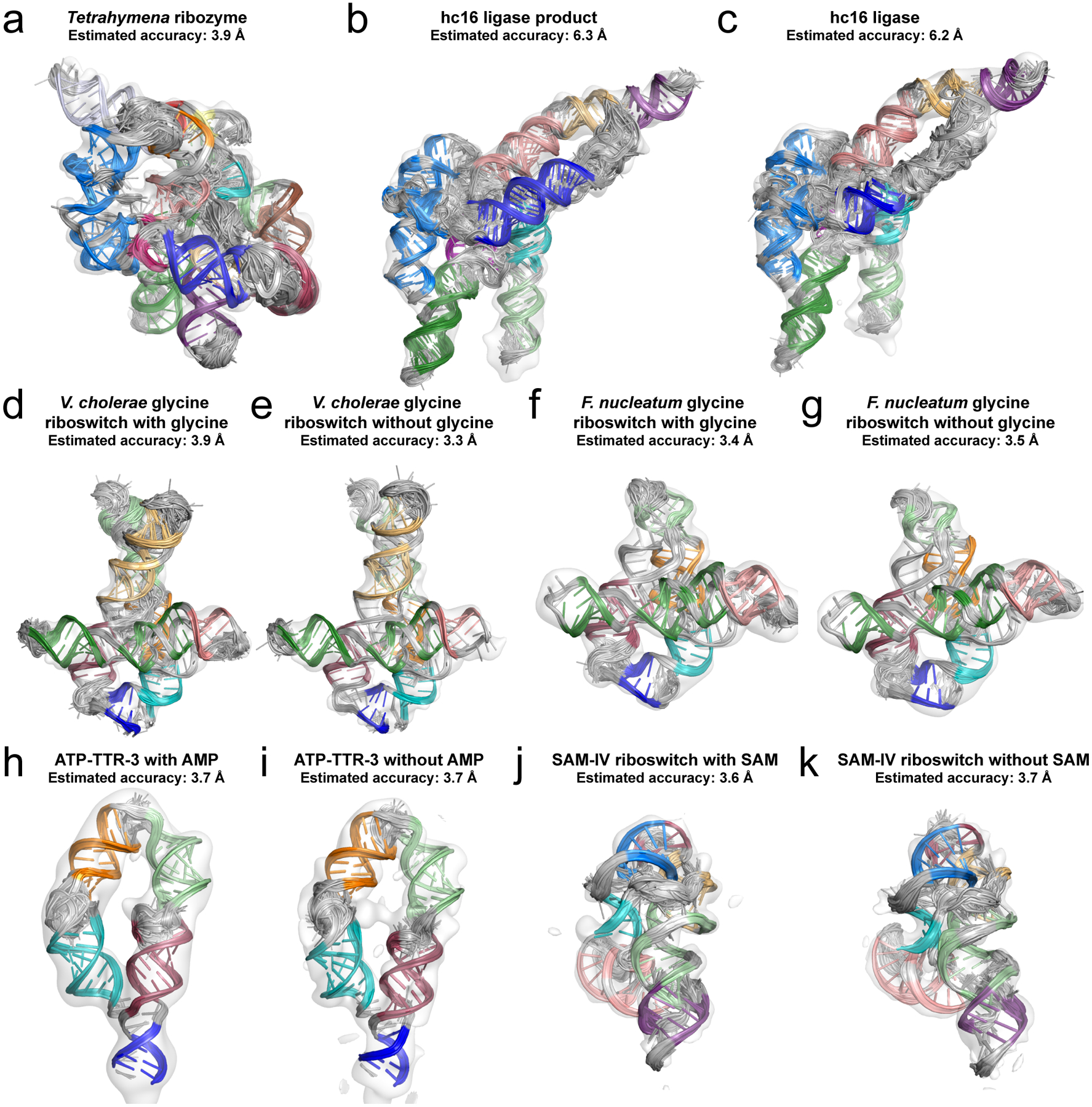
(A-K) Top scoring auto-DRRAFTER models in the cryo-EM maps and estimated accuracies based on modeling convergence. Each helix is depicted with a different bright color. Non-helical regions are colored gray.

Table 1.

Estimated accuracy of Ribosolve models^a

System	No. nts	Final no. particles used for 3D reconstruction	Map resolution (Å)	Estimated accuracya (Å)
Tetrahymena ribozyme	388	74,621	6.8	3.9
hc16 product	349	29,191	10.	6.3
hc16	338	21,263	11.	6.2
V. cholerae glycine riboswitch with glycine	231	193,317	5.7	3.9
V. cholerae glycine riboswitch apo	231	230,891	4.8	3.3
F. nucleatum glycine riboswitch with glycine	171	35,578	7.4	3.4
F. nucleatum glycine riboswitch apo	171	20,269	10.	3.5
ATP-TTR-3 with AMP	130	39,136	9.6	3.7
ATP-TTR-3 apo	130	71,045	10.	3.7
SAM-IV riboswitch with SAM	119	225,303	4.8	3.6
SAM-IV riboswitch apo	119	260,244	4.7	3.7

^aAccuracy is estimated from the modeling convergence (accuracy = 0.61 × convergence + 2.4), where convergence is defined as the average pairwise RMSD of the top ten scoring models built into half map 1 vs. models built into half map 2 (see Methods).

The F. nucleatum and V. cholerae glycine riboswitch Ribosolve models agreed well with the previously solved crystal structures^20,22 with mean RMSDs over the top scoring models of 4.9 Å for the F. nucleatum glycine riboswitch with glycine and 3.3 Å and 3.6 Å for the V. cholerae glycine riboswitch with and without glycine, respectively (Fig. 4A, B). These accuracies agreed well with predicted accuracies for these models based on DRRAFTER modeling convergence, supporting the relationship for accuracy estimation derived from simulation benchmarks (orange, Fig. 1C). For the Tetrahymena ribozyme, models were built starting from the previously solved crystal structure of the core of the ribozyme. The complete Tetrahymena ribozyme Ribosolve models fit well in the density map (Fig. 4C, D, Supplementary Table 4).

Fig. 4. Tests of Ribosolve model accuracy.

Top ten scoring fully automated Ribosolve models (models #2–10 are transparent; left; each helix depicted with a different bright color; non-helical regions colored gray), previously solved crystal structures (middle; colors match Ribosolve models), and overlay (right; Ribosolve models colored pink, crystal structure colored cyan) for (A) F. nucleatum glycine riboswitch and (B) V. cholerae glycine riboswitch. Note that auto-DRRAFTER models were built for the complete RNAs, but for clarity only the parts that correspond to the previously solved crystal structures are shown. (C) The Tetrahymena ribozyme Ribosolve model in the cryo-EM map. The region derived from a previously solved crystal structure is colored red and regions built de novo are colored black. (D) Real-space correlation between the Tetrahymena ribozyme Ribosolve models and cryo-EM map. Colors are the same as in (C). Real-space correlation values for each of the top ten scoring models built into each half map are shown as light blue lines, the average over all top scoring models is plotted as a thick blue line (n = 20 independent models). (E) The hc16 product Ribosolve model. Invariant and highly variable residues across final sequences from the original in vitro selection¹² shown as red and white spheres, respectively. The site of substrate ligation, the phosphorus atom in residue 1, is shown as a large blue sphere. All other residues are colored gray. (F) M2-seq Z-score plots (left) with putative tertiary contacts circled in red and Ribosolve models with nucleotides corresponding to the circled regions in the Z-score plots shown as red spheres for the ATP-TTR-3 with AMP (n = 914892 sequences). (G) The best-case SAM-IV apo state Ribosolve models built into the 4.7 Å cryo-EM map determined here (left, models #2–10 are transparent; each helix depicted with a different bright color; non-helical regions colored gray) and a 3.7 Å map³¹ (middle, colors match Ribosolve models). Models are shown overlaid on the right (Ribosolve models built into the 4.7 Å and 3.7 Å maps colored pink and cyan, respectively). (H) The fully automated SAM-IV apo state Ribosolve model with nucleotides hypothesized to form the SAM binding pocket shown as red spheres. Homologous nucleotides taken from a previously solved SAM-I riboswitch structure (PDB ID: 2GIS) are overlaid and shown as blue spheres.

For hc16 and the hc16 product, we confirmed that the Ribosolve models were consistent with all previous observations of the ribozyme¹². First, the models exhibited the P7 and P9 helices, which each contain nucleotides that exhibited covariation in clones examined from the original in vitro selection experiments. Nucleotides that were invariant across the final in vitro selected sequences are shown as red spheres in Fig. 4E and were all automatically modeled as near the substrate binding site or forming base pairs with regions of fixed sequence in the selection libraries. Nucleotides that were not conserved between sequences are shown as white spheres in Fig. 4E and did not make any interactions with other parts of the ribozyme in the Ribosolve model. Additionally, removing the thirteen nucleotides at the 3’ end of the ribozyme abolished its activity. In the Ribosolve model, most of these nucleotides are part of the P10, P10-ext, or P12 stems in the core of the structure.

The M2-seq data for the ATP-TTR-3 with and without AMP molecules contained features that were not explained by the M2-seq-derived secondary structures and appeared to correspond to tertiary contacts, providing additional information about nucleotides that should be close together in the three-dimensional structures (Fig. 4F, Supplementary Figure 3). We confirmed that our Ribosolve models, which were built without using this information, recovered these tertiary contacts (Fig. 4F, Supplementary Figure 3).

Finally, we compared our SAM-IV riboswitch models to Ribosolve models built into higher resolution density maps, which were obtained by collecting more data (3.7 Å for the apo state and 4.1 Å for the SAM bound state)³¹. The models agreed well with RMSDs of 3.8 Å for the apo state (Fig. 4G) and 2.5 Å for the SAM bound state. Additionally, six nucleotides in the SAM-IV riboswitch were previously hypothesized to form the binding pocket for SAM¹⁵. We confirmed that these nucleotides were all located near each other in the fully automated apo SAM-IV Ribosolve models, which were not built using this information, and that the conformation of these nucleotides was in good agreement with the conformation of putatively homologous nucleotides in the previously solved crystal structure of the SAM-I riboswitch (RMSD = 3.3 Å, Fig. 4H). Additionally, the best-case models for SAM-IV with and without SAM, which were built using this homology (see Methods for details), agreed with the fully automated models (RMSD = 5.0 Å and 5.6 Å for best-case models with and without SAM, respectively, vs. fully automated models without SAM).

The coordinate accuracy length scale achieved by Ribosolve (3.3–6.3 Å) is finer than the typical distance between backbone atoms in consecutive nucleotides and, historically, has been sufficient to attain non-trivial insights into whether RNAs of similar function have similar folds, how RNA structures respond to binding partners, and whether designed RNA structures fold as predicted^23,25,32,33. Each of the eleven Ribosolve models revealed at least one of these kinds of insights.

Glycine riboswitches from different species adopt nearly identical folds

The F. nucleatum and V. cholerae glycine riboswitches each contain two glycine aptamers that interact through tertiary contacts to form a butterfly-like fold (Fig. 3D–G, Fig. 5A)^20,22. For both RNAs, we observed evidence of two features predicted from previous computational analysis, a P0 stem (Fig. 3D–G, blue) and a kink-turn formed between the 5′ ends of each molecule and the linker between each molecule’s two glycine aptamers³⁴. In addition to the structural homology between the glycine riboswitches from different organisms, the two aptamers within each riboswitch also adopted nearly identical folds (Fig. 5A–B). Furthermore, for both riboswitches, the ligand-free states closely resemble the ligand-bound states (Fig. 3D–G). This invariance in tertiary fold upon ligand binding has been observed previously for other natural riboswitches and hypothesized for glycine riboswitches^34,35, but was not established for these glycine riboswitches because sequences previously used for structure determination were over-truncated^20,22.

Fig. 5. Functional insights from Ribosolve models.

(A) Overlay of V. cholerae and F. nucleatum glycine riboswitches with glycine. Aptamer 1 is colored light pink and light green for the F. nucleatum and V. cholerae glycine riboswitches, respectively. Aptamer 2 is colored pink and green for the F. nucleatum and V. cholerae glycine riboswitches, respectively. (B) Overlay of both glycine aptamers from the F. nucleatum and V. cholerae structures. Models are colored as in (A). (C-D) Structural homology between the SAM-IV riboswitch and SAM-I and SAM-I/IV riboswitches. (C) The SAM-I crystal structure³⁷, the SAM-I/IV crystal structure³⁶, and the SAM-IV Ribosolve model, and (D) an overlay of all three structures, with the core colored cyan, and peripheral elements shown as gray transparent ribbons. SAM is shown as transparent red spheres. (E) Comparisons of Ribosolve structures for ATP-TTR-3 with and without AMP, colored dark and light purple, respectively, and the computationally designed models, colored gray. (F) The overall architecture of the previously predicted model of the Tetrahymena ribozyme³⁸ (core and peripheral elements colored light orange and orange, respectively) qualitatively matches the Ribosolve structure (core and peripheral elements colored light blue and blue, respectively), with peripheral elements wrapping around the core. The Ribosolve structure contains holes (arrows in middle panel) not present in the predicted structure. (G) Comparison of the hc16 Ribosolve structures without substrate (pink) and with ligated substrate (gray). The substrate-binding segment and substrate are highlighted in red and black, respectively.

Distinct peripheral architectures support a conserved core structure across multiple classes of SAM riboswitches

Ribosolve revealed that the SAM-IV riboswitch adopts a complex fold with two pseudoknots (Fig. 3J, K). Comparison of this structure with previously solved crystal structures of SAM-I and SAM-I/IV riboswitches showed that the tertiary structure is substantially rewired across the three classes of SAM riboswitches (Fig. 5C), but the core structures are nearly identical in all three molecules (Fig. 5D)^36,37. These observations are consistent with previously hypothesized homology based on secondary structure³⁶. Like the glycine riboswitches, the apo and holo SAM-IV riboswitch structures are highly similar (Fig. 3J, K).

Assessing the model accuracy of computationally designed RNA molecules

Beyond its application to determining structures of natural RNAs, Ribosolve enabled rapid assessment of the synthetic ATP-TTR-3 structure. ATP-TTR-3 embeds the AMP aptamer into a clothespin-like scaffold, which was designed to pre-organize the aptamer structure and enhance its ligand binding affinity¹⁷, analogous to natural riboswitch aptamers, including the glycine and SAM riboswitches solved above (Fig. 3D–G, J–K). Automated Ribosolve structures of ATP-TTR-3 with and without AMP confirmed this pre-folding into the computer-designed tertiary structures within the estimated coordinate error (RMSDs of 4.2 Å and 4.3 Å, respectively) (Fig. 5E). Additionally, the ATP-TTR-3 Ribosolve structures with and without AMP are very similar (mean RMSD = 2.7 Å), further supporting the hypothesis that minimal conformational rearrangement occurs upon ligand binding (Fig. 5E).

The complete global architecture of the Tetrahymena ribozyme and rearrangements of core elements in the hc16 ligase

Ribosolve structures of our two largest molecules offered comparisons to literature predictions and to each other. First, the Tetrahymena ribozyme is a paradigmatic RNA enzyme discovered 38 years ago and manually modeled 24 years ago³⁸ (Fig. 3A). Peripheral elements of the ribozyme, P2, P2.1, P9.2, P9.1, P13, P14, are resolved for the first time here; these elements wrap around the core of the ribozyme, to complete a ring around its catalytic core, substantiating a decades-old qualitative prediction (Fig. 5F), while also revealing large holes in the structure that were not previously predicted (Fig. 5F, arrows)³⁸. Second, the hc16 ribozyme is a ligase evolved in vitro from a random library that contained the P4-P6/P3-P8 domain of the Tetrahymena ribozyme as a constant scaffold region¹²; it was expected that the architecture of the hc16 ligase would be very similar to the Tetrahymena ribozyme. Instead, the hc16 Ribosolve structure exhibits a unique extended conformation that has not yet been observed in other ribozyme structures (Fig. 3B, C). In both the structures without substrate and with ligated substrate, the active site is at the center of the hc16 molecule and the substrate-binding segment is positioned like the string of a bow (Fig. 5G). This rearrangement of the hc16 ligase from its ‘parent’ Tetrahymena ribozyme, while unexpected, provides a rationalization for observations in prior sequence conservation data for hc16, is consistent with new chemical mapping data for the RNA (Supplementary Text; Supplementary Figure 4), and provides an illustration of how unbiased structure determination enabled by Ribosolve can refine structure-function-homology relationships.

Limitations of the Ribosolve pipeline

Ribosolve has significant advantages over previous RNA-only structure determination techniques, most notably, the relative speed and ease with which the technique can be applied and its applicability to RNA molecules that have been refractory to crystallography and NMR, such as the Tetrahymena ribozyme. However, when applying Ribosolve, it is important to be mindful of its limitations (Fig. 6). First, although Ribosolve always produces an ensemble of all-atom models, it does not provide atomic scale structural detail (Fig. 6A). We do not expect even the most highly converged Ribosolve models to correctly position all atoms. Such models may contain register shifts or other systematic inaccuracies. Ensembles of several independently generated models, visualized as ribbons rather than as atom-level coordinates, should be reported to convey the precision of the method. Accuracy estimates based on this model convergence place additional bounds on the level of structural detail that should be interpreted. Second, because Ribosolve accuracy estimates do not take map resolution into account, we caution against building models into maps that do not clearly exhibit RNA-like features, particularly major and/or minor helical grooves. These models may still converge tightly, resulting in underestimation of model uncertainty. To illustrate this limitation, we built models into a 12 Å Spinach-TTR-3 map and a 14 Å Eterna3D-JR_1 map generated from the data collected for these systems, for which the 2D class averages exhibited substantial heterogeneity and the 3D reconstructions did not show obvious RNA features (Extended Data Figure 4). In each case, the models converged tightly, resulting in putative accuracy estimates of 4.2 Å for Spinach-TTR-3 and 3.9 Å for Eterna3D-JR_1 (Fig. 6B). These accuracy estimates are similar to those for our other eleven Ribosolve models, despite the additional uncertainty arising from the lower resolution maps. Furthermore, the models for Eterna3D-JR_1 do not contain a tertiary contact for which there is evidence in the M2-seq data (Extended Data Figure 7L), suggesting that these models may be inaccurate. A third limitation of the Ribosolve pipeline results from the fact that auto-DRRAFTER modeling relies on accurate secondary structure information. Models built with inaccurate secondary structures can often be identified by visual inspection¹⁰. For example, models of hc16 built with the incorrect secondary structure did not fit well in the density map (Fig. 6C). In these cases, additional mutate-map-rescue experiments^39,40 may be required to determine and/or validate the correct secondary structure. Finally, Ribosolve models should always be independently validated. Here, we validated each model by comparing to crystallographic conformations of sub-structures, comparing to functional and/or biochemical data, or by performing mutate-map-rescue experiments (Fig. 4). The necessary validation will depend both on the system and the questions being asked.

Fig. 6. Limitations of the Ribosolve pipeline.

(A) Though Ribosolve produces all-atom models, it does not provide atomic resolution detail. Indeed, the atomic details of Ribosolve models are often incorrect (top right). A ribbon-and-basepair representation of the ensemble of top scoring models (below) better depicts the approximately nucleotide-resolution of most Ribosolve models. The F. nucleatum glycine riboswitch with glycine is shown here. Ribosolve models are colored blue and the previously solved crystal structure is colored gray. Regions of the Ribosolve models that were not previously crystallized are not shown for clarity. (B) Highly converged Eterna3D-JR_1 models built into a 14 Å density map. The estimated accuracy of these models is 3.9 Å, but does not account for additional uncertainty due to the poor resolution of the density map. We do not recommend building models into density maps that do not contain visually identifiable RNA helices. (C) (Top) Models of the hc16 product built with the incorrect secondary structure do not fit well in the density map. (Bottom) With the correct secondary structure, auto-DRRAFTER builds models that fit well in the density map. Models are colored blue and maps colored gray in (B) and (C).

Many of these limitations could potentially be resolved by improving the cryo-EM map resolution. The main RNA features visible in the cryo-EM maps resolved here (all maps are > 4 Å resolution) are overall fold and major and minor grooves, which enable visualization of conformational rearrangements, structural homology, and validation of designed structures. At higher resolution more detailed features would be visible. Around 3–4 Å resolution, some base pairs may be visible, but the connectivity of the backbone is typically less clear. At approximately 3.0 Å resolution, individual RNA bases, base pairs, phosphates, and metal ions are visible. At this resolution, atomic details can typically be inferred, enabling detailed visualization of noncanonical interactions and interactions with small molecules. Here, there is a correlation between the amount of cryo-EM data collected and the final map resolution (r² = 0.82 for map resolution vs. number of particles, two-tailed p = 0.0001, N=11), suggesting that the resolution of many of these maps could possibly be improved by collecting more data. Indeed, we showed that the maps of the SAM-IV riboswitch with and without SAM could be improved from 4.8 Å and 4.7 Å to 4.1 Å and 3.7 Å , respectively³¹. However, the cryo-EM B-factors for SAM-IV with and without SAM were lower than for many of the other RNAs, suggesting that such an improvement in map resolution may not be possible for all of the RNA maps determined here (Supplementary Table 1). Additionally, even with the higher resolution SAM-IV maps, auto-DRRAFTER was still used to build models because manual coordinate modeling was not possible. In this case, substantial further improvement in map resolution was not possible. It would require approximately 50x the number of particles to get a 3.0 Å resolution map for SAM-IV³¹. For other RNAs in this study, such improvement in map resolution may require even more data, up to 50–1000 times the current amount. As application of cryo-EM to RNA-only systems becomes more common, it is likely that some maps will reach resolutions of 3 Å or better, but we also expect that many maps will be in the resolution range where the full Ribosolve pipeline, including M2-seq and auto-DRRAFTER modeling, will be required.

Discussion

The Ribosolve pipeline combines recent advances in cryo-EM, M2-seq biochemical analysis, and Rosetta auto-DRRAFTER computer modeling to accelerate three-dimensional RNA structure determination. Using this method, we determined 3D models of eleven RNA molecules, including riboswitches, ribozymes, and synthetic RNA nanostructures, over the timescale of months (Fig. 1D). Several independent tests including a blind challenge, internal controls that had been previously solved by crystallography, and independent biochemical experiments validate and confirm the Ribosolve models. The resolution, while not reaching atomic precision, is sufficient to reveal global tertiary structural features, to detect structural rearrangements upon target binding, to confirm or refute hypotheses of homology between RNA classes, and to validate structure predictions for designed nanostructures. Use of the Rosetta auto-DRRAFTER tool, rather than manual coordinate modeling, accelerates model building into maps and also enables estimation of model accuracy from modeling convergence. Studies on the T-box and SAM-IV riboswitches from our group occurring in parallel or as follow-up to this work further support the utility and accuracy of cryo-EM and automated modeling to solve RNA 3D structures^30,31. Important frontiers for Ribosolve include inference of RNA conformational ensembles rather than single dominant conformations⁴¹; automatic refinement of RNA secondary structures during 3D model building, which may obviate M2-seq experiments; acceleration of auto-DRRAFTER, which will be needed for completely automatic modeling of larger RNA assemblies; model refinement techniques to improve the accuracy of Ribosolve models; systematic benchmarking of the relationship between the amount of cryo-EM data collected and final map resolution for RNA-only systems; and systematic tests of RNAs with a wider range of lengths and varying numbers of tertiary contacts.

Online Methods

RNA preparation

DNA templates for all molecules except Tetrahymena ribozyme were prepared by PCR assembly of DNA oligonucleotides designed with Primerize⁴² and purchased from Integrated DNA Technologies (Supplementary Table 5). DNA templates were purified with AMPure XP beads (Beckman Coulter) following the manufacturer’s instructions. RNA was then prepared by in vitro transcription from these DNA templates, then purified with Zymo RNA Clean and Concentrator columns (Zymo Research) following the manufacturer’s instructions. Complete details of the RNA preparation, including preparation of the Tetrahymena ribozyme RNA, are provided in Supplementary Note 1.

After preparing the RNA, we confirmed that the three ribozymes in our benchmark set (Tetrahymena ribozyme, hc16, and 24–3) were catalytically active (Supplementary Figure 5). We performed activity assays as previously described^12,13 with fluorescently labeled RNA substrates, and ran gels to check that the appropriate products were generated. Complete details are provided in Supplementary Note 2.

Native gels

All native gels were run using a BioRad Criterion Cell gel cassette. Polyacrylamide gels were cast by combining 15 mL of 8% or 12% 29:1 acrylamide:bis, in 10 mM MgCl₂, 67 mM HEPES, 33 mM Tris, pH 7.2 solution with 150 μL 10% ammonium persulfate and 30 μL TEMED. After the gel polymerized, chilled buffer containing 33 mM Tris, 10 mM MgCl₂, 67 mM HEPES, pH 7.2 was added and the gel apparatus was placed in an ice bath in a 4 °C cold room. Folded RNA was prepared as follows. 1 μg of RNA was diluted to a volume of 6.4 μL, then incubated at 90°C for 3 minutes, then room temperature for 10 minutes. 0.8 μL of 500 mM Na-HEPES pH 8 and 0.8 μL of 100 mM MgCl2 was added, then the reaction was incubated at 50°C for 20 minutes, and finally for 10 minutes at room temperature. All RNAs were screened in the apo state. 2 μL of loading buffer containing 250 mM Na-HEPES pH 7.5, 5 mM EDTA pH 8, 50% glycerol, 0.05% xylene cyanol, and 0.05% bromophenol blue was then added and samples were then loaded into the gel immediately. The gel was run at 10 W for 1.5 hours. The temperature of the gel was monitored closely to avoid overheating. To visualize the RNA, the gel was submerged in Stains-All working solution (0.015% dye in 45% formamide) and placed on an orbital shaker for 25 minutes. The Stains-All solution was then removed and the gel was de-stained in water for 15 minutes. The water was then removed and the gel was imaged.

M2-seq experiments

M2-seq experiments were performed as previously described²⁹. Complete details are provided in Supplementary Note 3.

Cryo-EM sample preparation

RNAs were prepared as follows. RNAs were combined with Na-HEPES, pH 8.0 and incubated at 90°C for 3 minutes, then cooled at room temperature for 10 minutes. MgCl₂ and any ligands were added and the solution was incubated at 50 °C for 20 minutes (30 minutes for Tetrahymena ribozyme), then cooled at room temperature for 10 minutes. The final concentrations were 10 mM MgCl₂, 50 mM Na-HEPES, pH 8.0. The final RNA and ligand concentration were: 15 μM Tetrahymena ribozyme RNA; 15 μM hc16 product RNA; 15 μM hc16 RNA; 25 μM scaRNA6 RNA; 25 μM V. cholerae glycine riboswitch RNA and 100 mM glycine; 15 μM V. cholerae glycine riboswitch RNA; 21 μM RB1 5′ UTR RNA; 25 μM U1 snRNA RNA; 25 μM 24–3 RNA; 13 μM F. nucleatum glycine riboswitch RNA and 100 mM glycine; 17 μM F. nucleatum glycine riboswitch RNA; 20 μM Eterna3D-JR_1 RNA; 26 μM spinach-TTR-3 RNA; 27 μM ATP-TTR-3 RNA and 1 mM AMP; 30 μM ATP-TTR-3 RNA; 40 μM SAM-IV riboswitch RNA and 1 mM SAM; 45 μM SAM-IV riboswitch RNA; 40 μM downstream peptide riboswitch RNA and 10 mM glutamine.

Cryo-EM data collection

Three microliters of the samples were applied onto glow-discharged 200-mesh R2/1 or R3.5/1 Quantifoil grids. The grids were blotted for 2–4 s and flash frozen in liquid ethane using a Vitrobot Mark IV (Thermo Fisher Scientific) with the chamber cooled to 4 °C and 100% humidity. The Tetrahymena ribozyme, hc16, hc16 product, RB1 5’ UTR RNA, U1 snRNA RNA, F. nucleatum glycine riboswitch with and without glycine, Eterna3D-JR_1 RNA, spinach-TTR-3 RNA, ATP-TTR-3 with and without AMP, and downstream peptide riboswitch with glutamine were imaged on a Talos Arctica cryo-electron microscope with a Volta phase plate. Between 600 and 1,414 micrographs were collected for each sample. The scaRNA6 and 24–3 RNAs were imaged on a f with GIF energy filter (Gatan), without a phase plate, and 860 and 2,260 micrographs were collected, respectively. Initial datasets of approximately 500 images (23,000 particles) for the apo SAM-IV riboswitch and 900 images (20,000 particles) for the apo V. cholerae glycine riboswitch were collected on a Talos Arctica cryo-electron microscope with a Volta phase plate and a JEOL ARM300 cryo-electron microscope with a hole free phase plate, respectively. We performed 2D analysis as described below and confirmed that RNA helices could be identified in the 2D class averages before collecting additional data. We did not collect similar initial datasets for the SAM-IV riboswitch with SAM nor for the V. cholerae glycine riboswitch with glycine because we assumed that the data quality would be similar with and without the substrates. We then collected larger datasets for the SAM-IV riboswitch with and without SAM and the V. cholerae glycine riboswitch with and without glycine on a Titan Krios cryo-electron microscope with GIF energy filter, without a phase plate. All micrographs were recorded by EPU software (Thermo Fisher Scientific) with a Gatan K2 Summit direct electron detector, where each image was composed of 30 individual frames with an exposure time of 6 s. All images were collected with defocus between −0.5 μm and −3.5 μm.

Cryo-EM image processing

All micrographs were motion corrected using MotionCor2⁴³ version 1.2.1 and the contrast transfer function (CTF) was determined using CTFFIND4⁴⁴ version 4.1.13. All particles were autopicked using the NeuralNet option in EMAN2⁴⁵ version 2.3, and further checked manually to select additional good particles that were missed and also to remove some bad particles. Then, particle coordinates were imported to Relion⁴⁶ version 3.0.2, where the 2D classification was performed. Several rounds of 2D classification were performed to remove poor 2D classes without clear RNA features. After 2D classification, we performed 3D reconstruction with cryoSPARC⁴⁷ version 2.0.20, Relion⁴⁷ version 3.0.2, and EMAN2⁴⁵ version 2.3. For each RNA, the software that produced the highest resolution map was used to generate the final map. In summary, for the SAM-IV riboswitch with and without SAM, V. cholerae glycine riboswitch with and without glycine, RB1 5′ UTR, U1 snRNA, Eterna3D-JR_1, and spinach-TTR-3, scaRNA6, and 24–3 ribozyme, we used cryoSPARC⁴⁷, including 3D initial model building and classification with the “Ab initio reconstruction” option, and 3D refinement using the “homogeneous refinement” option. For the Tetrahymena ribozyme, hc16 ligase, hc16 ligase product, F. nucleatum glycine riboswitch with and without glycine, ATP-TTR-3 with and without AMP, and downstream peptide riboswitch with glutamine, we used EMAN2 to build the 3D initial model using “e2initialmodel.py”, then performed 3D classification and final 3D refinement in Relion. Additional information about the data collection and image processing, including the initial and final numbers of particles, can be found in Supplementary Table 1. A representative example of the data processing workflow is shown for the apo state of the V. cholerae glycine riboswitch in Extended Data Figure 3. Local map resolution was calculated with ResMap (Extended Data Figure 5)⁴⁸.

Auto-DRRAFTER pipeline

The auto-DRRAFTER software is freely available to academic users as part of the Rosetta software suite at www.rosettacommons.org. Documentation is available at https://www.rosettacommons.org/docs/latest/application_documentation/rna/auto-drrafter and a demo is available at https://www.rosettacommons.org/demos/latest/public/auto-drrafter/README. A limited version of the software is also freely available through an online ROSIE server at https://rosie.rosettacommons.org/auto-drrafter.

The auto-DRRAFTER pipeline is illustrated in Extended Data Figure 6. The inputs to auto-DRRAFTER were an RNA sequence, secondary structure, and cryo-EM map and the output was a collection of 3D models of the RNA structure. The auto-DRRAFTER pipeline begins by representing both the map and secondary structure as graphs to enable automated placement of at least one RNA helix in the density map (Extended Data Figure 6A–C). This process may result in multiple possible helix placements. For each of these, the rest of the RNA was then built with RNA fragment assembly in Rosetta, keeping the placed helix fixed throughout the run⁴⁹. The low-resolution and all-atom Rosetta score functions were augmented with the elec_dens_fast score term to monitor agreement with the density map⁵⁰.

Modeling was performed in several rounds (Extended Data Figure 6C–J). For each round, 1000 models (for the simulated benchmark) or 2000 models (for the models built into experimental maps) were built for each placement. The average pairwise RMSD (convergence) was then computed for the top ten scoring models across all helix placements. If the convergence RMSD was higher than 10 Å, then another round of modeling was performed. Elements of the structure that had converged and fit well in the density map in the previous round of modeling were then kept fixed for the subsequent modeling round. When the convergence of the top ten scoring models across all possible helix placements dropped below 10 Å, two final rounds of modeling were performed in which the conformations of the converged regions were refined while poorly converged regions continued to be modeled de novo. The last modeling round was performed in parallel in separate half maps, if available. The total numbers of modeling rounds performed for all RNAs described here are listed in Table 1, Supplementary Table 2, and Supplementary Table 6. One round of modeling took approximately one day on 50 × (number of helix placements) cores (Intel Xeon E5–2640v4 processors). The complete details of the auto-DRRAFTER pipeline are described in the Supplementary Note 4. Figures were prepared with Pymol and UCSF Chimera⁵¹.

Auto-DRRAFTER benchmark on simulated maps

Starting with the database of nonredundant RNA PDB structures (release 3.39) solved to 4.0 Å resolution or better⁵², we found all RNA structures of length between 100 and 450 nucleotides, then removed structures with protein or DNA residues, multiple chains, and/or many missing residues. This yielded 25 structures, from which we selected a set of eight functionally and structurally diverse RNAs: THF riboswitch (PBD ID: 3SUX)⁵³, c-di-AMP riboswitch (PDB ID: 4QK8)⁵⁴, bacterial SRP Alu domain (PDB: 4WFL)⁵⁵, FMN riboswitch (PDB ID: 3F2Q)⁵⁶, SAM-I riboswitch (PDB ID: 4KQY)⁵⁷, Tetrahymena ribozyme P4-P6 domain (PDB ID: 1GID)⁵⁸, lysine riboswitch (PDB ID: 3DIL)⁵⁹, and the lariat capping ribozyme (PDB ID: 4P8Z)⁶⁰. Density maps were simulated at 10 Å resolution with EMAN2 using the following command:

e2pdb2mrc.py crystal_structure.pdb simulated_map.mrc --res=10.0 --center

We then built models with auto-DRRAFTER starting from the RNA sequences, secondary structures derived from the crystal structures, and simulated density maps. Fragments from homologous RNA structures were excluded during the fragment assembly stages of the auto-DRRAFTER runs with the following flags:

-fragment_homology_rmsd 1.2 -exclusion_match_type MATCH_YR
-exclude_fragment_files crystal_structure.pdb

where crystal_structure.pdb is the previously solved crystal structure. RMSDs between auto-DRRAFTER models and the crystal structure were calculated over all heavy atoms (all atoms except hydrogens) after alignment over all heavy atoms.

For the THF riboswitch, we also built models into the 2.9 Å crystallographic density map. Models were built as described above, but with the crystallographic density substituted for the simulated density map.

HIV-1 DIS blind modeling challenge

Models for the HIV-1 DIS dimer were built with multiple different strategies using an early version of auto-DRRAFTER that required manually placing at least one helix in the cryo-EM density map and in which all modeling was performed in a single round¹⁰. The complete details are provided in Supplementary Note 5.

T-box-tRNA complex modeling

Models of the B. subtilis T-box-tRNA complex were built into a 4.9 Å cryo-EM map using auto-DRRAFTER. Three helices were initially fit into the density map (tRNA residues 1–7, 65–71, 38–42, 26–30, 33–35 and T-box residues 99–101). These initial placements were automatically optimized throughout the modeling process. Five rounds of auto-DRRAFTER modeling were performed. RMSD accuracies were calculated by comparing to the published model, which was based on high-resolution crystal structures³⁰.

Fully automated and ‘best-case’ models for experimental density maps

Automated models were built for all experimental density maps using the auto-DRRAFTER method as described above with secondary structures derived from our M2-seq experiments. Additionally, we built a set of best-case auto-DRRAFTER models for these same systems which integrated prior information with the cryo-EM and M2-seq data to generate models of potentially higher accuracy. For this set of models, the M2-seq-based secondary structures were modified based on sequence covariation information and previously solved crystal structures (Extended Data Figure 8). Additionally, specific elements of the RNA structures were initially placed in the density maps rather than using the automatic helix placement strategy described above. These elements were allowed to move from their initial positions during all rounds of modeling. A complete description of this modeling is provided in Supplementary Note 6.

Auto-DRRAFTER error estimates and model validation

To estimate model error, we calculated the auto-DRRAFTER modeling convergence, defined as the average pairwise RMSD over the top ten scoring auto-DRRAFTER models. Models were not aligned before computing RMSDs. All RMSDs reported in this work are computed over all atoms except hydrogens. For models built into half maps, the convergence was defined as the average pairwise RMSD between the top ten scoring models refined into each of the half maps. For models built into a single map, convergence can be calculated in Rosetta with the following command:

drrafter_error_estimation -s <models> -rmsd_nosuper

For models built into separate half maps, convergence can be calculated with the command:

drrafter_error_estimation -sgroup1 <models1> -sgroup2 <models2> -rmsd_nosuper

where models1 and models2 are the top ten scoring models refined into the two separate half maps.

Modeling convergence correlates with model accuracy (r² = 0.95 for the benchmark on simulated maps, two-tailed p = 9×10⁻²⁹, N=45), with a best-fit line of y = 0.61x + 2.4. This linear relationship was used to predict model accuracy for all models built into experimental density maps. Per-residue convergence was similarly calculated over the top ten scoring models and also correlates with per-residue model accuracy (r² = 0.88 for the benchmark on simulated maps, two-tailed p < 0.001, N = 6357), with a best-fit line of y = 0.75x + 2.0. Real-space correlation coefficients over the full model and per residue were calculated in Rosetta with the following command⁶¹:

density_tools -s <model> -mapfile <density map> -mapreso <map resolution> -cryo-EM_scatterers -denstools::perres

RMSD accuracies relative to higher resolution coordinates were computed over all heavy atoms. Mean RMSDs were calculated as the mean of the RMSDs of each of the top ten scoring Ribosolve models built into separate half maps, if available, relative to the higher resolution coordinates.

Statistics

All cryo-EM statistics are reported in Supplementary Table 1. Auto-DRRAFTER modeling statistics are reported in Supplementary Table 2, Supplementary Table 3, and Supplementary Table 6. We used auto-DRRAFTER to build 2000 models per round for each RNA for which we had an experimental density map, and 1000 models per round for simulated density maps. The numbers of rounds of modeling are provided in Supplementary Table 2, Supplementary Table 3, and Supplementary Table 6. Pearson’s correlation coefficients (r²) are reported with the exact N values used for calculations. All p-values reported are two-tailed.

hc16 mutate-map-rescue experiments

All mutate-map-rescue experiments were performed as previously described on the hc16 product construct used for the M2-seq experiments³⁹. Details are provided in Supplementary Note 7.

Data availability

Cryo-EM maps are available in the EMDB with accession codes EMD-21831, EMD-21832, EMD-21833, EMD-21834, EMD-21835, EMD-21836, EMD-21838, EMD-21839, EMD-21840, EMD-21841, and EMD-21842. Models (best-case) are available in the PDB with accession codes 6WLJ, 6WLK, 6WLL, 6WLM, 6WLN, 6WLO, 6WLQ, 6WLR, 6WLS, 6WLT, and 6WLU. Fully automated models are available in the supplementary data. M2-seq and mutate-map-rescue data is available in the RMDB with accession codes RB1UTR_DMS_0000, 243RNA_DMS_0000, ATPAPO_DMS_0000, ATPAMP_DMS_0000, U1SNRNA_DMS_0000, SCARNA6_DMS_0000, VCKTAPO_DMS_0000, VCKTGLY_DMS_0000, DPRGLN_DMS_0000, ETERNA3_DMS_0000, SPINACH_DMS_0000, FNKTAPO_DMS_0000, FNKTGLY_DMS_0000, HC16APO_DMS_0000, HC16PRO_DMS_0000, SAM4APO_DMS_0000, SAM4SAM_DMS_0000, L21RNA_DMS_0000, HC16M2R_1M7_0001, HC16M2R_1M7_0002, HC16M2R_1M7_0003. The data that support the findings of this study are available from the corresponding author upon request.

Code availability

The auto-DRRAFTER software is freely available to academic users as part of the Rosetta software package. Documentation is available at https://www.rosettacommons.org/docs/latest/application_documentation/rna/auto-drrafter and a demo is available at https://www.rosettacommons.org/demos/latest/public/auto-drrafter/README. A limited version of the software is also freely available through an online ROSIE server at https://rosie.rosettacommons.org/auto-drrafter.

Materials and correspondence

Correspondence and requests for materials should be addressed to Rhiju Das (rhiju@stanford.edu) or Wah Chiu (wahc@stanford.edu).

Extended Data

Extended Data Fig. 1. Native gel screens for all RNAs in this study.

Gel images for (1) and (2) RB1 5′ UTR, (3) and (4) scaRNA6, (5) and (6) U1 snRNA, (7) and (8) SAM-IV riboswitch (apo), (9) and (10) 24–3, (11) V. cholerae glycine riboswitch (apo), (12) hc16, (13) Tetrahymena ribozyme, (14) F. nucleatum glycine riboswitch (apo), (15) and (16) Eterna3D-JR_1, (17) and (18) spinach-TTR-3, (19) F. nucleatum glycine riboswitch (apo), (20) ATP-TTR-3 (apo), (21) Eterna3D-JR_1, (22) SAM-IV riboswitch (apo), (23) downstream peptide riboswitch, (24) hc16, and (25) hc16 product. Samples 1–13, 24, 25 were run on an 8% polyacrylamide gel. Samples 14–23 were run on a 12% polyacrylamide gel. All samples were run in 10 mM MgCl₂, 67 mM HEPES, 33 mM Tris, pH 7.2. All gels that were run are shown here (experiments were not repeated beyond results shown here).

Extended Data Fig. 2. Representative micrographs for all RNAs in this study.

Micrographs shown in (A), (B), (C), (G), (H), (I), (J), (K), (L), (O), (Q), and (R) were taken with the Talos Arctica. All others were taken with the Titan Krios. A Volta phase plate was used for (A), (B), (C), (G), (H), (I), (J), (K), (L), (O), and (Q). The total numbers of micrographs collected are listed in Table S1.

Extended Data Fig. 3. Example cryo-EM data processing workflow.

Shown here for the V. cholerae glycine riboswitch without glycine.

Extended Data Fig. 4. Cryo-EM 2D class averages and 3D reconstructions for all RNA systems in this study.

One dataset was collected for all RNAs except for the SAM-IV riboswitch without SAM and V. cholerae glycine riboswitch without glycine, for which smaller preliminary datasets were initially collected (see Methods). Results from these preliminary datasets were similar, though map resolution was lower. The numbers of particles used for the 3D reconstructions are listed in Table S1.

Extended Data Fig. 5. Local cryo-EM map resolution for RNA-only structures.

Calculated with ResMap⁴⁸ for (A) Tetrahymena ribozyme, (B) hc16 product, (C) hc16, (D) V. cholerae glycine riboswitch with glycine, (E) V. cholerae glycine riboswitch without glycine, (F) F. nucleatum glycine riboswitch with glycine, (G) F. nucleatum glycine riboswitch without glycine, (H) ATP-TTR-3 with AMP, (I) ATP-TTR-3 without AMP, (J) SAM-IV riboswitch with SAM, and (K) SAM-IV riboswitch without SAM.

Extended Data Fig. 6. auto-DRRAFTER overview.

The F. nucleatum glycine riboswitch is shown here as an example. (A) Secondary structure elements that connect to just one other helix or junction (“end nodes”) are circled. (B) The cryo-EM density map is low-pass filtered to 20 Å and points are placed (spheres) throughout the map to identify possible placements for “end nodes” in the map (red spheres). The circled end node was randomly selected for initial helix placement. A probe helix (black) was then fit into the density map. The location of the probe helix was optimized, while the distances between the C1’ atom of nucleotide 6 (nucleotides 1–6 labeled) of the probe helix (black sphere) and the end node and the neighboring map node were monitored (see Supplementary Note 4). (C) 3D models are built for each of the elements circled in (A) and fit into the density map in the location of the circled point in (B). These elements are kept fixed while the rest of the RNA is built into the density map. (D) The top ten best scoring models after round 1. The overall convergence of these models is above the 10 Å threshold (convergence = 20.2 Å), so another round of modeling is performed. (E) For the second round of modeling, regions that have converged are extracted from the top scoring models and kept fixed while the rest of the RNA is built into the density map. (F) The top ten scoring models after round 2. The convergence is below the 10 Å threshold (convergence = 6.2 Å), so there is only one initial model for the third round of modeling, composed of converged regions from the top ten scoring models from round 2 (G). These regions are allowed to move from their initial positions during this modeling round. (H) The best scoring models from round 3. (I) Again, converged regions are extracted from top scoring models to form the initial model for the final round of modeling. These regions are kept fixed during the fragment assembly stage of auto-DRRAFTER modeling, but allowed to move during final refinement. (J) The top ten scoring models built independently into each half map. Helical regions are depicted with bright colors in (C)-(J) and match colors in the secondary structure diagram (A). Non-helical regions are colored gray.

Extended Data Fig. 7. Experimental M2-seq Z-score plots.

(A) Tetrahymena ribozyme (n = 65041 sequences), (B) hc16 product (n = 459852 sequences), (C) hc16 (n = 451568 sequences), (D) human scaRNA6 (n = 866158 seqeunces), (E) V. cholerae glycine riboswitch with glycine (n = 928767 sequences), (F) V. cholerae glycine riboswitch without glycine (n = 974343 sequences), (G) human RB1 5′ UTR (n = 889700 sequences), (H) 24–3 (n = 515486 sequences), (I) human U1 snRNA (n = 1185187), (J) F. nucleatum glycine riboswitch with glycine (n = 803254 sequences), (K) F. nucleatum glycine riboswitch without glycine (n = 670301 sequences), (L) eterna3D-JR_1 (n = 994048 sequences), (M) spinach-TTR-3 (n = 1090666 sequences), (N) ATP-TTR-3 with AMP (n = 914892 sequences), (O) ATP-TTR-3 without AMP (n = 712801 sequences), (P) SAM IV riboswitch with SAM (n = 131464 sequences), (Q) SAM IV riboswitch without SAM (n = 991972 sequences), and (R) downstream peptide riboswitch (n = 1012081 sequences).

Extended Data Fig. 8. Secondary structures automatically derived from M2-seq data and revisions for best-case auto-DRRAFTER modeling based on sequence covariation and previously solved crystal structures.

(A) Tetrahymena ribozyme, (B) hc16 product, (C) hc16, (D) V. cholerae glycine riboswitch with glycine, (E) V. cholerae glycine riboswitch without glycine, (F) F. nucleatum glycine riboswitch with glycine, (G) F. nucleatum glycine riboswitch without glycine, (H) ATP-TTR-3 with AMP (I) ATP-TTR-3 without AMP, (J) SAM-IV riboswitch with SAM, and (K) SAM-IV riboswitch without SAM. (A-K) Blue lines indicate base pairs that are present in the best-case, but not automated secondary structures. Red lines indicate base pairs that are present in the automated, but not best-case secondary structures. (L) The previously proposed hc16 secondary structure⁴. (M) M2-seq and mutate-map-rescue experiments suggest that hc16 contains alt-P4 rather than P4. (N) Additional modeling and experiments suggest further modifications to the hc16 secondary structure: alt-P4 is extended, a pseudoknot is formed between the hairpin loops of P5c and P1, P5 is not formed, and P10 is formed. Helical regions are depicted with bright colors that match those shown in Fig. 3. Non-helical regions are colored black.

Extended Data Fig. 9. Secondary structures for best-case Ribosolve models.

(A) Tetrahymena ribozyme, (B) hc16 product, (C) hc16, (D) V. cholerae glycine riboswitch with glycine, (E) V. cholerae glycine riboswitch without glycine, (F) F. nucleatum glycine riboswitch with glycine, (G) F. nucleatum glycine riboswitch without glycine, (H) eterna3D-JR_1 (see Fig. 6), (I) spinach-TTR-3 (discussed in “Limitations of the Ribosolve pipeline” in the main text), (J) ATP-TTR-3 with AMP (K) ATP-TTR-3 without AMP, (L) SAM-IV riboswitch with SAM, and (M) SAM-IV riboswitch without SAM. Helical regions are depicted with bright colors that match those shown in Fig. 3. Non-helical regions are colored black.

Extended Data Fig. 10. Benchmarking auto-DRRAFTER accuracy.

(A-H) The top ten scoring auto-DRRAFTER models (models #2–10 are transparent) built into 10 Å simulated density maps (left) and the corresponding crystal structures (right) for (A) THF riboswitch, (B) c-di-AMP riboswitch, (C) bacterial SRP Alu domain, (D) FMN riboswitch, (E) SAM-I riboswitch, (F) Tetrahymena ribozyme P4-P6 domain, (G) lysine riboswitch, and (H) lariat capping ribozyme. (I) Ribosolve models for THF riboswitch built into the previously solved 2.9 Å crystallographic density map (left) and the crystal structure (right). (J) Ribosolve models for the B. subtilis T-box-tRNA complex built into a 4.9 Å cryo-EM map (left) and previously modeled coordinates based on high-resolution crystal structures³⁰. Helical regions are depicted with bright colors. Non-helical regions are colored gray.

References

- 1.Atkins JF, Gesteland RF & Cech T RNA worlds: from life’s origins to diversity in gene regulation. (Cold Spring Harbor Laboratory Press; New York;, 2011). [Google Scholar]
- 2.Cech TR & Steitz JA The Noncoding RNA Revolution-Trashing Old Rules to Forge New Ones. Cell 157, 77–94, doi: 10.1016/j.cell.2014.03.008 (2014). [DOI] [PubMed] [Google Scholar]
- 3.Birney E et al. Identification and analysis of functional elements in 1% of the human genome by the ENCODE pilot project. Nature 447, 799–816, doi: 10.1038/nature05874 (2007). [DOI] [PMC free article] [PubMed] [Google Scholar]
- 4.Zhang JW & Ferre-D’Amare AR New molecular engineering approaches for crystallographic studies of large RNAs. Curr Opin Struc Biol 26, 9–15, doi: 10.1016/j.sbi.2014.02.001 (2014). [DOI] [PMC free article] [PubMed] [Google Scholar]
- 5.Zhang H & Keane SC Advances that facilitate the study of large RNA structure and dynamics by nuclear magnetic resonance spectroscopy. Wiley Interdisciplinary Reviews: RNA, e1541 (2019). [DOI] [PMC free article] [PubMed] [Google Scholar]
- 6.Bergfors T Screening and optimization methods for nonautomated crystallization laboratories. Methods Mol Biol 363, 131–151, doi: 10.1007/978-1-59745-209-0_7 (2007). [DOI] [PubMed] [Google Scholar]
- 7.McMullan G, Faruqi AR, Clare D & Henderson R Comparison of optimal performance at 300 keV of three direct electron detectors for use in low dose electron microscopy. Ultramicroscopy 147, 156–163, doi: 10.1016/j.ultramic.2014.08.002 (2014). [DOI] [PMC free article] [PubMed] [Google Scholar]
- 8.Ognjenovic J, Grisshammer R & Subramaniam S Frontiers in Cryo Electron Microscopy of Complex Macromolecular Assemblies. Annu Rev Biomed Eng, doi: 10.1146/annurev-bioeng-060418-052453 (2019). [DOI] [PubMed] [Google Scholar]
- 9.Zhang KM et al. Structure of the 30 kDa HIV-1 RNA Dimerization Signal by a Hybrid Cryo-EM, NMR, and Molecular Dynamics Approach. Structure 26, 490–498 e493, doi: 10.1016/j.str.2018.01.001 (2018). [DOI] [PMC free article] [PubMed] [Google Scholar]
- 10.Kappel K et al. De novo computational RNA modeling into cryo-EM maps of large ribonucleoprotein complexes. Nature methods 15, 947 (2018). [DOI] [PMC free article] [PubMed] [Google Scholar]
- 11.Kruger K et al. Self-splicing RNA: autoexcision and autocyclization of the ribosomal RNA intervening sequence of Tetrahymena. Cell 31, 147–157 (1982). [DOI] [PubMed] [Google Scholar]
- 12.Jaeger L, Wright MC & Joyce GF A complex ligase ribozyme evolved in vitro from a group I ribozyme domain. Proceedings of the National Academy of Sciences 96, 14712–14717 (1999). [DOI] [PMC free article] [PubMed] [Google Scholar]
- 13.Horning DP & Joyce GF Amplification of RNA by an RNA polymerase ribozyme. Proceedings of the National Academy of Sciences 113, 9786–9791 (2016). [DOI] [PMC free article] [PubMed] [Google Scholar]
- 14.Mandal M et al. A glycine-dependent riboswitch that uses cooperative binding to control gene expression. Science 306, 275–279, doi:DOI 10.1126/science.1100829 (2004). [DOI] [PubMed] [Google Scholar]
- 15.Weinberg Z et al. The aptamer core of SAM-IV riboswitches mimics the ligand-binding site of SAM-I riboswitches. Rna-a Publication of the Rna Society 14, 822–828, doi: 10.1261/rna.988608 (2008). [DOI] [PMC free article] [PubMed] [Google Scholar]
- 16.Ames TD & Breaker RR Bacterial aptamers that selectively bind glutamine. Rna Biol 8, 82–89, doi: 10.4161/rna.8.1.13864 (2011). [DOI] [PMC free article] [PubMed] [Google Scholar]
- 17.Yesselman JD et al. Computational design of three-dimensional RNA structure and function. Nat Nanotechnol 14, 866–873, doi: 10.1038/s41565-019-0517-8 (2019). [DOI] [PMC free article] [PubMed] [Google Scholar]
- 18.Paige JS, Wu KY & Jaffrey SR RNA Mimics of Green Fluorescent Protein. Science 333, 642–646, doi: 10.1126/science.1207339 (2011). [DOI] [PMC free article] [PubMed] [Google Scholar]
- 19.Lee J et al. RNA design rules from a massive open laboratory. P Natl Acad Sci USA 111, 2122–2127, doi: 10.1073/pnas.1313039111 (2014). [DOI] [PMC free article] [PubMed] [Google Scholar]
- 20.Huang LL, Serganov A & Patel DJ Structural Insights into Ligand Recognition by a Sensing Domain of the Cooperative Glycine Riboswitch. Molecular Cell 40, 774–786, doi: 10.1016/j.molcel.2010.11.026 (2010). [DOI] [PMC free article] [PubMed] [Google Scholar]
- 21.Guo F, Gooding AR & Cech TR Structure of the Tetrahymena ribozyme: Base triple sandwich and metal ion at the active site. Molecular Cell 16, 351–362, doi: 10.1016/S1097-2765(04)00592-1 (2004). [DOI] [PubMed] [Google Scholar]
- 22.Butler EB, Xiong Y, Wang J & Strobel SA Structural basis of cooperative ligand binding by the glycine riboswitch. Chem Biol 18, 293–298, doi: 10.1016/j.chembiol.2011.01.013 (2011). [DOI] [PMC free article] [PubMed] [Google Scholar]
- 23.Golden BL, Gooding AR, Podell ER & Cech TR A preorganized active site in the crystal structure of the Tetrahymena ribozyme. Science 282, 259–264, doi:DOI 10.1126/science.282.5387.259 (1998). [DOI] [PubMed] [Google Scholar]
- 24.Marz M et al. Animal snoRNAs and scaRNAs with exceptional structures. Rna Biol 8, 938–946, doi: 10.4161/rna.8.6.16603 (2011). [DOI] [PMC free article] [PubMed] [Google Scholar]
- 25.Krummel DAP, Oubridge C, Leung A, Li JD & Nagai K Crystal Structure of a Ten-Subunit Human Spliceosomal U1 snRNP at 5.5 angstrom Resolution. Biophysical Journal 100, 198–198 (2011).21190672 [Google Scholar]
- 26.Kutchko KM et al. Multiple conformations are a conserved and regulatory feature of the RB1 5 ‘ UTR. Rna 21, 1274–1285, doi: 10.1261/rna.049221.114 (2015). [DOI] [PMC free article] [PubMed] [Google Scholar]
- 27.Russel D et al. Putting the Pieces Together: Integrative Modeling Platform Software for Structure Determination of Macromolecular Assemblies. Plos Biol 10, doi: 10.1371/journal.pbio.1001244 (2012). [DOI] [PMC free article] [PubMed] [Google Scholar]
- 28.Ovchinnikov S et al. Large-scale determination of previously unsolved protein structures using evolutionary information. Elife 4, doi: 10.7554/eLife.09248 (2015). [DOI] [PMC free article] [PubMed] [Google Scholar]
- 29.Cheng CY, Kladwang W, Yesselman JD & Das R RNA structure inference through chemical mapping after accidental or intentional mutations. P Natl Acad Sci USA 114, 9876–9881, doi: 10.1073/pnas.1619897114 (2017). [DOI] [PMC free article] [PubMed] [Google Scholar]
- 30.Li S et al. Structural basis of amino acid surveillance by higher-order tRNA-mRNA interactions. Nat Struct Mol Biol, doi: 10.1038/s41594-019-0326-7 (2019). [DOI] [PMC free article] [PubMed] [Google Scholar]
- 31.Zhang K et al. Cryo-EM Structure of a 40-kDa SAM-IV Riboswitch RNA at 3.7 Å Resolution. Nat Commun (In press.). [DOI] [PMC free article] [PubMed] [Google Scholar]
- 32.Schmitt E et al. Structure of the ternary initiation complex aIF2-GDPNP-methionylated initiator tRNA. Nat Struct Mol Biol 19, 450–454, doi: 10.1038/nsmb.2259 (2012). [DOI] [PubMed] [Google Scholar]
- 33.Lane SW et al. Construction and Crystal Structure of Recombinant STNV Capsids. J Mol Biol 413, 41–50, doi: 10.1016/j.jmb.2011.07.062 (2011). [DOI] [PubMed] [Google Scholar]
- 34.Kladwang W, Chou FC & Das R Automated RNA Structure Prediction Uncovers a Kink-Turn Linker in Double Glycine Riboswitches. Journal of the American Chemical Society 134, 1404–1407, doi: 10.1021/ja2093508 (2012). [DOI] [PubMed] [Google Scholar]
- 35.Cheng CY et al. Consistent global structures of complex RNA states through multidimensional chemical mapping. Elife 4, doi: 10.7554/eLife.07600 (2015). [DOI] [PMC free article] [PubMed] [Google Scholar]
- 36.Trausch JJ et al. Structural basis for diversity in the SAM clan of riboswitches. P Natl Acad Sci USA 111, 6624–6629, doi: 10.1073/pnas.1312918111 (2014). [DOI] [PMC free article] [PubMed] [Google Scholar]
- 37.Montange RK & Batey RT Structure of the S-adenosylmethionine riboswitch regulatory mRNA element. Nature 441, 1172–1175, doi: 10.1038/nature04819 (2006). [DOI] [PubMed] [Google Scholar]
- 38.Lehnert V, Jaeger L, Michel F & Westhof E New loop-loop tertiary interactions in self-splicing introns of subgroup IC and ID: A complete 3D model of the Tetrahymena thermophila ribozyme. Chemistry & Biology 3, 993–1009, doi:Doi 10.1016/S1074-5521(96)90166-0 (1996). [DOI] [PubMed] [Google Scholar]
- 39.Tian SQ, Cordero P, Kladwang W & Das R High-throughput mutate-map-rescue evaluates SHAPE-directed RNA structure and uncovers excited states. Rna 20, 1815–1826, doi: 10.1261/rna.044321.114 (2014). [DOI] [PMC free article] [PubMed] [Google Scholar]
- 40.Tian S, Kladwang W & Das R Allosteric mechanism of the V. vulnificus adenine riboswitch resolved by four-dimensional chemical mapping. Elife 7, doi: 10.7554/eLife.29602 (2018). [DOI] [PMC free article] [PubMed] [Google Scholar]
- 41.Zhao DQ & Jardetzky O An Assessment of the Precision and Accuracy of Protein Structures Determined by Nmr - Dependence on Distance Errors. J Mol Biol 239, 601–607, doi:DOI 10.1006/jmbi.1994.1402 (1994). [DOI] [PubMed] [Google Scholar]
- 42.Tian S, Yesselman JD, Cordero P & Das R Primerize: automated primer assembly for transcribing non-coding RNA domains. Nucleic Acids Research 43, W522–W526, doi: 10.1093/nar/gkv538 (2015). [DOI] [PMC free article] [PubMed] [Google Scholar]
- 43.Zheng SQ et al. MotionCor2: anisotropic correction of beam-induced motion for improved cryo-electron microscopy. Nature Methods 14, 331–332, doi: 10.1038/nmeth.4193 (2017). [DOI] [PMC free article] [PubMed] [Google Scholar]
- 44.Rohou A & Grigorieff N CTFFIND4: Fast and accurate defocus estimation from electron micrographs. J Struct Biol 192, 216–221, doi: 10.1016/j.jsb.2015.08.008 (2015). [DOI] [PMC free article] [PubMed] [Google Scholar]
- 45.Tang G et al. EMAN2: An extensible image processing suite for electron microscopy. J Struct Biol 157, 38–46, doi: 10.1016/j.jsb.2006.05.009 (2007). [DOI] [PubMed] [Google Scholar]
- 46.Scheres SHW RELION: Implementation of a Bayesian approach to cryo-EM structure determination. J Struct Biol 180, 519–530, doi: 10.1016/j.jsb.2012.09.006 (2012). [DOI] [PMC free article] [PubMed] [Google Scholar]
- 47.Punjani A, Rubinstein JL, Fleet DJ & Brubaker MA cryoSPARC: algorithms for rapid unsupervised cryo-EM structure determination. Nature Methods 14, 290-+, doi: 10.1038/Nmeth.4169 (2017). [DOI] [PubMed] [Google Scholar]
- 48.Kucukelbir A, Sigworth FJ & Tagare HD Quantifying the local resolution of cryo-EM density maps. Nature Methods 11, 63–65, doi: 10.1038/Nmeth.2727 (2014). [DOI] [PMC free article] [PubMed] [Google Scholar]
- 49.Das R, Karanicolas J & Baker D Atomic accuracy in predicting and designing noncanonical RNA structure. Nat Methods 7, 291–294, doi: 10.1038/nmeth.1433 (2010). [DOI] [PMC free article] [PubMed] [Google Scholar]
- 50.DiMaio F & Chiu W Tools for Model Building and Optimization into Near-Atomic Resolution Electron Cryo-Microscopy Density Maps. Resolution Revolution: Recent Advances in Cryoem 579, 255–276, doi: 10.1016/bs.mie.2016.06.003 (2016). [DOI] [PMC free article] [PubMed] [Google Scholar]
- 51.Pettersen EF et al. UCSF chimera - A visualization system for exploratory research and analysis. Journal of Computational Chemistry 25, 1605–1612, doi: 10.1002/jcc.20084 (2004). [DOI] [PubMed] [Google Scholar]
- 52.Leontis NB & Zirbel CL in RNA 3D Structure Analysis and Prediction (eds Leontis Neocles & Westhof Eric) 281–298 (Springer; Berlin Heidelberg, 2012). [Google Scholar]
- 53.Huang L, Ishibe-Murakami S, Patel DJ & Serganov A Long-range pseudoknot interactions dictate the regulatory response in the tetrahydrofolate riboswitch. Proc Natl Acad Sci U S A 108, 14801–14806, doi: 10.1073/pnas.1111701108 (2011). [DOI] [PMC free article] [PubMed] [Google Scholar]
- 54.Gao A & Serganov A Structural insights into recognition of c-di-AMP by the ydaO riboswitch. Nat Chem Biol 10, 787–792, doi: 10.1038/Nchembio.1607 (2014). [DOI] [PMC free article] [PubMed] [Google Scholar]
- 55.Kempf G, Wild K & Sinning I Structure of the complete bacterial SRP Alu domain. Nucleic Acids Research 42, 12284–12294, doi: 10.1093/nar/gku883 (2014). [DOI] [PMC free article] [PubMed] [Google Scholar]
- 56.Serganov A, Huang LL & Patel DJ Coenzyme recognition and gene regulation by a flavin mononucleotide riboswitch. Nature 458, 233–U210, doi: 10.1038/nature07642 (2009). [DOI] [PMC free article] [PubMed] [Google Scholar]
- 57.Lu CR et al. SAM Recognition and Conformational Switching Mechanism in the Bacillus subtilis yitJ S Box/SAM-I Riboswitch. J Mol Biol 404, 803–818, doi: 10.1016/j.jmb.2010.09.059 (2010). [DOI] [PMC free article] [PubMed] [Google Scholar]
- 58.Cate JH et al. Crystal structure of a group I ribozyme domain: Principles of RNA packing. Science 273, 1678–1685, doi: 10.1126/science.273.5282.1678 (1996). [DOI] [PubMed] [Google Scholar]
- 59.Serganov A, Huang LL & Patel DJ Structural insights into amino acid binding and gene control by a lysine riboswitch. Nature 455, 1263–U1276, doi: 10.1038/nature07326 (2008). [DOI] [PMC free article] [PubMed] [Google Scholar]
- 60.Meyer M et al. Speciation of a group I intron into a lariat capping ribozyme. P Natl Acad Sci USA 111, 7659–7664, doi: 10.1073/pnas.1322248111 (2014). [DOI] [PMC free article] [PubMed] [Google Scholar]
- 61.Wang RYR et al. Automated structure refinement of macromolecular assemblies from cryo-EM maps using Rosetta. Elife 5, doi: 10.7554/eLife.17219 (2016). [DOI] [PMC free article] [PubMed] [Google Scholar]
Associated Data
This section collects any data citations, data availability statements, or supplementary materials included in this article.
Supplementary Materials
Data Availability Statement