Robust entanglement of an asymmetric quantum dot molecular system in a Josephson junction

Abstract

We demonstrate the generation of robust entanglement of a quantum dot molecular system in a voltage-controlled junction. To improve the quantum information characteristics of this system, we propose an applicable protocol which contains the implementation of asymmetric quantum dots as well as the engineering of reservoirs. Quantum dots can provide asymmetric coupling coefficients due to the tunable energy barriers through the gap voltage changes. To engineer the reservoirs, superconducting leads are used to prepare a voltage-biased Josephson junction. The high-controllability properties of this system give the arbitrary magnitude of entanglement by the arrangement of parameters. Significantly, the perfect entanglement can be achieved for an asymmetric structure in response to the increase of bias voltage, and also it continues saturated with the near-unit amount.

Quantum mechanics; Quantum dot molecule; Quantum entanglement; Quantum transport; Superconductors; Josephson junction

1. Introduction

Recent advancements in condensed matter physics and nanotechnology open new possibilities for the implementation of nanodevices in quantum information studies. Although, the concept of entanglement was basically studied for distinguishable bipartite systems [1], [2], [3], [4], [5], in recent years there has been a great deal of interest in quantifying the entanglement of indistinguishable components in condensed matter systems. The elements of these systems are identical massive particles which involve quantum correlations at short distances. The entanglement of indistinguishable particles either bosons or fermions should be characterized with their symmetrized or antisymmetrized wave functions respectively [6], [7], [8], [9], [10], [11], [12], [13]. Particularly, the entanglement of fermions in condensed matter systems can be evaluated by two methods: entanglement of modes [8], [12], [14], [15] and entanglement of particles [6], [7], [9], [10], [11]. In the former, the entanglement of indistinguishable fermions is associated with the shared modes not particles of subsystems in single-particle Hilbert space. But for the latter, the entanglement of fermions specifically is concerned about the antisymmetrization of quantum wave functions of indistinguishable fermionic particles.

For fermionic entanglement of particles, firstly the quantum correlations of two fermions in a 2K dimensional single-particle space were characterized [6]. After that more than two indistinguishable particles, fermions in higher-dimensional single-particle spaces were analyzed and quantum correlations of pure states in the arbitrary-dimensional Hilbert space were classified [7]. Recently, a multipartite concurrence was introduced for N-indistinguishable fermionic particles in an arbitrary-dimensional pure states [11]. It was presented that the multipartite concurrence can be displayed as an average amount of one observable when two copies of the compound state are accessible.

For studying the entanglement of indistinguishable fermionic particles, quantum dots (QDs) [16], [17] can be taken into account as promising candidates. QDs as one branch of broad two-state qubit systems [18] play prominent roles in nanostructures for their tunable discrete energy levels and also for their easy controllability of barriers by gate voltages.

Also, quantum dot molecules (QDMs) consist of quantum dots which are coupled by tunneling and separated by barriers have received great attention theoretically and experimentally [19], [20], [21], [22]. These quantum structures have been selected as the ideal choices for researching in quantum information processing. The analysis of entanglement dynamics between two electrons inside coupled quantum molecules demonstrated the crucial entanglement characteristics [23].

Theoretical [24] and experimental [25] studies showed that the asymmetric structure of quantum molecules has enhanced the control of tunneling features. It was theoretically shown that in an asymmetric quantum dot molecular system, the fidelity of entangled photon pairs can be achieved near-unit magnitude [26]. In addition, the asymmetric quantum dot-lead couplings have been extensively implemented in electrical [27] and thermal [28] rectification devices to improve the electric and heat transport technologies.

Moreover, superconducting devices have found impressive interest in quantum information setups [29], [30] because of their long intrinsic coherency with no dissipation characteristics. Recent years, employing the superconducting qubits and superconducting resonators have improved the exploring of quantum entanglement [31], [32], quantum teleportation [33], [34] and quantum computing [35], [36] studies. Superconducting qubits namely phase [37], flux [38] and charge [39] qubits can be connected with microwave [40], electrical [41], mechanical [42], and superconducting [43] resonators.

According to the frequency range of superconducting devices, these nanostructures would be driven by microwave [44], [45] or optical [46], [47] fields. Also, QDs in normal biased-voltage junctions have extensively been used experimentally [48], [49], [50] and theoretically [51], [52], [53]. Recently, quantum transport through the QDs system in contact with Josephson junctions (JJs) which act as the single transistors to filter the transfer of electrons has attracted a great deal of attention [54], [55], [56], [57], [58].

It seems that quantum information studies on an asymmetric quantum dot molecule in a bias-controlled Josephson junction can be considered as an interesting area for research which can provide novel achievements. Therefore in this study, we propose a QDM system in a conventional JJ with asymmetric tunneling coefficients to achieve robust entanglement and also to keep its magnitude near-unit under the bias voltage control. To this end, we consider the indistinguishable entanglement for our system which becomes possible by evaluating the fermionic concurrence. To explore the quantum information processing of QDM system in a biased-voltage junction, we perform our analysis in Markovian regime. First, we obtain the quantum transport of molecular system to show the current-voltage characteristics (I-V) as one of the important properties of biased-voltage circuits. Then, we investigate the control of the entanglement with respect to the bias voltage. We find that with only bias voltage control, the complete controllability to yield perfect entanglement is not possible. Therefore, we apply the strategy of left-right asymmetric coupling strength to achieve robust entanglement. The dynamics of entanglement and its response to bias voltage in different situations of symmetric and asymmetric couplings demonstrate wide flexibility of the proposed setup to provide a desired high entanglement. The main advantage of this molecular system includes the feasible controlling elements of the easy-tunable bias voltage driving field and the manipulation of quantum dot couplings. Indeed by engineering reservoirs and the presence of superconducting leads, the performance of the system is extensively influenced to provide robustly entangled states.

This paper is organized as follows: In Sec. 2, we introduce the proposed model composed of a quantum dot molecular system in a JJ by describing the whole Hamiltonian. We compute the quantum transport of our molecular system in Sec. 3. In Sec. 4 by introducing symmetric and asymmetric structures, we obtain the entanglement of QDM system under the bias voltage control. In Sec. 5, we present the results of the entanglement behavior in bias voltage changes and its time evolution in constant bias voltages and also for specific order parameters. Finally, we conclude the results in Sec. 6.

2. Model

The proposed open quantum system consists of a QDM weakly coupled to the superconducting leads which is demonstrated in Fig. 1, schematically. Applying an external bias voltage between the leads L and R induces the electron transport from the left to the right. The Hamiltonian of the whole system can be written as:

$$\hat{H}={\hat{H}}_{QDM}+{\hat{H}}_{Leads}+{\hat{H}}_{int}.$$ (1)

For simplicity, the polarized molecular quantum dot system is taken in spinless Anderson-Holstein model [59], [60]. So, ${\hat{H}}_{QDM}$, the Hamiltonian of quantum dot molecule is expressed as:

$${\hat{H}}_{QDM}=\sum _{\alpha }{\epsilon }_{\alpha }{\hat{d}}_{\alpha }^{\mathrm{†}}{\hat{d}}_{\alpha }+t_{AB}({\hat{d}}_A^{\mathrm{†}}{\hat{d}}_B+{\hat{d}}_A{\hat{d}}_B^{\mathrm{†}}),$$ (2)

here, ${\hat{d}}_{\alpha }^{\mathrm{†}}({\hat{d}}_{\alpha })$ is the creation (annihilation) operator of quantum dot $\alpha =A,B$ with electronic energy levels ${\epsilon }_{\alpha }$. Beyond the Coulomb blockade regime with the condition of $k_{B}T\ll E_C$ ($E_C$ is the charging energy), single-electron tunneling is dominant for each QD [61], [62]. In the second term, $t_{AB}$ describes the inter-dot hopping strength which can be tuned using an applied gate voltage. In Eq. (1), ${\hat{H}}_{Leads}$ which introduce the Hamiltonian of left and right superconducting leads are described by the mean-field Hamiltonian as [63], [64]:

$${\hat{H}}_{Leads}^{MF}=\sum _{k\nu \sigma }{\xi }_{k\nu }{\hat{c}}_{k\nu \sigma }^{\mathrm{†}}{\hat{c}}_{k\nu \sigma }+\sum _{k\nu }({\mathrm{\Delta }}_{\nu }{\hat{c}}_{k\nu \uparrow }^{\mathrm{†}}{\hat{c}}_{-k\nu \downarrow }^{\mathrm{†}}+{\mathrm{\Delta }}_{\nu }^{⁎}{\hat{c}}_{-k\nu \downarrow }{\hat{c}}_{k\nu \uparrow }).$$ (3)

Here, ${\hat{c}}_{k\nu \sigma }^{\mathrm{†}}({\hat{c}}_{k\nu \sigma })$ is the creation (annihilation) operator of an electron with momentum k and spin $\sigma =\uparrow ,\downarrow$ in lead $\nu =L,R$. In this relation, ${\xi }_{k\nu }={\epsilon }_k-{\mu }_{\nu }$ is the particle energy in which ${\epsilon }_k$ denotes the single-particle energy regards to the electrochemical potential ${\mu }_{\nu }$. Moreover, ${\mathrm{\Delta }}_{\nu }=|{\mathrm{\Delta }}_{\nu }|e^{i{\varphi }_{\nu }}$ remarks the superconducting energy gap of lead ν with the superconducting phase, ${\varphi }_{\nu }$. The mean field Hamiltonian could be diagonalized by applying Bogoliubov transformation which is presented in Supplementary Material (1). This procedure leads to obtain:

$${\hat{H}}_{Leads}=E_G+\sum _{k\nu \sigma }{E}_{\nu k}{\hat{\gamma }}_{k\nu \sigma }^{\mathrm{†}}{\hat{\gamma }}_{k\nu \sigma },$$ (4)

where $E_G$, the ground state energy, represents the Cooper pair condensate energy and ${\hat{\gamma }}_{k\nu \sigma }^{\mathrm{†}}({\hat{\gamma }}_{k\nu \sigma })$ denotes the creation (annihilation) operator of Bogoliubov fermionic quasiparticle excitation which are used for diagonalizing the Hamiltonian of superconducting leads. The interaction Hamiltonian, ${\hat{H}}_{int}$ in Eq. (1), corresponds to the tunneling between the QDs and electrodes which can be written as:

$${\hat{H}}_{int}=\sum _{k\nu \alpha }(T_{k\nu \alpha }{\hat{c}}_{k\nu }^{\mathrm{†}}{\hat{d}}_{\alpha }+T_{k\nu \alpha }^{⁎}{\hat{c}}_{k\nu }{\hat{d}}_{\alpha }^{\mathrm{†}}).$$ (5)

The tunneling coefficient, $T_{k\nu \alpha }$, describes the coupling strength depending on k, the momentum of an electron in lead ν, the site of quantum dot α.

Figure 1.

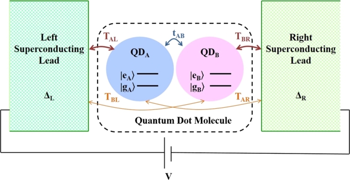
The proposed physical system: A quantum dot molecule system consists of two coupled quantum dots, A and B, with inter-dot coupling strength t_AB and QD-lead coupling strengths: T_AL, T_AR, T_BR, T_BL. The superconducting leads with the superconducting energy gaps Δ_L and Δ_R are under the bias voltage V.

To determine the temperature region of the present quantum dot molecule, we consider all temperature conditions of this system. The required temperature for the entanglement of particles such as atoms and quantum dots [65], [66] and also the transition temperature of superconductivity for the low-temperature as well as high-temperature superconductors [67]show that our proposed setup may work well from a few Kelvin. Concerning the difficulties of overcoming the quantum decoherence and to preserve the entanglement, we suppose that the range of mili Kelvin would be more realistic.

To investigate the time evolution of the system, the quantum master equation (QME) is obtained. This derivation is shown in the Supplementary Materials (2). Then, we calculate the electric current and entanglement in the following sections. As in this paper only the electric current is investigated, for convenience, we drop the electric and use current instead of the electric current expression.

3. Current

To have transport through the present system, an external bias voltage is applied to the electrodes shown in Fig. 1. Due to this asymmetric bias voltage V, the density of states of reservoirs are changed such that the electrochemical potential of the left lead becomes ${\mu }_L\to {\mu }_0+eV$ while the right one remains as ${\mu }_R={\mu }_0$ which is illustrated in Fig. 2. This means that $eV={\mu }_L-{\mu }_R$. It leads to moving electrons from the left reservoir to the QDM and then to the right lead. Consequently, it causes a flowing current through the junction.

Figure 2.

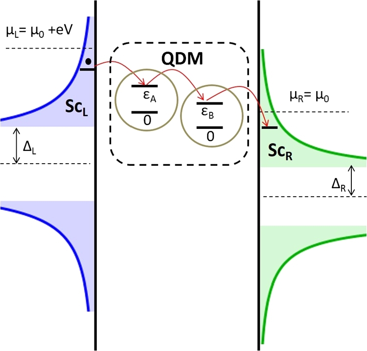
The density of states in the superconducting reservoirs of Sc_L/QDM/Sc_R junction. The asymmetric applied bias voltage, eV = μ_L − μ_R, lets carriers to flow from the left reservoir to the QDM and then to the right lead.

Current as a measurable quantity denotes the variation of total charged particle number in the lead ν which is defined as [57], [68]:

$${\hat{I}}_{\nu }(t)=-e\frac{d{\hat{N}}_{\nu }}{dt}=\frac{ie}{ħ}[{\hat{N}}_{\nu }(t),{\hat{H}}_I(t)]=\frac{ie}{ħ}\sum _{k\alpha }(T_{k\alpha }{\hat{c}}_{k\nu }^{\mathrm{†}}{\hat{d}}_{\alpha }-T_{k\alpha }^{⁎}{\hat{c}}_{k\nu }{\hat{d}}_{\alpha }^{\mathrm{†}}),$$ (6)

where ${\hat{N}}_{\nu }={\sum }_{\nu }{\hat{c}}_{\nu }^{\mathrm{†}}{\hat{c}}_{\nu }$ is the number of electric charge e. According to the QME formalism, the density matrix evolution of the system would be written as $\dot{\hat{\rho }}=\hat{M}\hat{\rho }$. In this relation matrix $\hat{M}$ shows the properties of the master equation. Therefore, we can rewrite the current formula, Eq. (6), as [58], [69]:

$${\hat{I}}_{\nu }(t)=\frac{e}{ħ}\langle \hat{N}|{\hat{M}}_{\nu }|\hat{\rho }(t)\rangle ,$$ (7)

where ${\hat{M}}_{\nu }$ shows the contribution of lead ν in matrix $\hat{M}$. In the steady-state of the system, by taking so long time ($t\to \infty$), the stationary transport is shown in Fig. 3 containing the plots of normal junction ($\mathrm{\Delta }=0$) and JJ with different energy gaps.

Figure 3.

Current-voltage characteristics in specific superconducting energy gaps. Normal leads: Solid line Δ = 0, Superconducting leads: Dashed line $\frac{\mathrm{\Delta }}{{\mathrm{\Gamma }}_0}=1.8$, Dot-dashed $\frac{\mathrm{\Delta }}{{\mathrm{\Gamma }}_0}=2.6$ for Γ₀ = πN_F|T|², $I_0=e\frac{{\mathrm{\Gamma }}_0}{ħ}$ and Δ_L = Δ_R = Δ.

According to the I-V characteristic curves which are shown in Fig. 3, the magnitude of current is growing by the increase of bias voltage. Only in energies equal to the quantum dots' energy levels, the current hits the peaks in delta type for the superconducting leads while it illustrates the smooth steps for the normal leads. Although the current level of the system is increased by raising the magnitude of energy gaps, it reaches the platform for the large enough bias voltage.

In all calculations to deal with only the quasiparticle transport and ignoring the Cooper pair current, we assume all energy levels are far enough from the order parameter of leads.

4. Concurrence

It is convenient to apply the concurrence as a measure of entanglement for two-qubit systems. In the following, first this measure of entanglement for two distinguishable qubits is defined. Then, fermionic concurrence for indistinguishable particles will be characterized and evaluated in analogue with Wootters' formula.

4.1. Concurrence of distinguishable particles

For the first time, Wootters introduced the measure of concurrence to evaluate the entanglement of qubits with two parties in both pure and mixed states [70], [71]. This measure of entanglement is defined as:

$$C(\rho )=Max[0,{\lambda }_1-{\lambda }_2-{\lambda }_3-{\lambda }_4],$$ (8)

in which, ${\lambda }_i,(i=1,2,3,4)$ represents the non-negative eigenvalues of a matrix $\hat{R}$ in decreasing order ${\lambda }_1>{\lambda }_2>{\lambda }_3>{\lambda }_4$. The matrix $\hat{R}$ is defined as:

$$\hat{R}=\sqrt{\sqrt{\hat{\rho }}\tilde{\hat{\rho }}\sqrt{\hat{\rho }}},$$ (9)

where $\hat{\rho }={\sum }_i{p}_i|{\psi }_i\rangle \langle {\psi }_i|$ denotes the density matrix of the system in which, $p_i$ is the probability of each state of decompositions. Also $\tilde{\hat{\rho }}=({\hat{\sigma }}_y\otimes {\hat{\sigma }}_y){\hat{\rho }}^{⁎}({\hat{\sigma }}_y\otimes {\hat{\sigma }}_y)$. In this relation, $\widehat{{\sigma }_y}$ describes the y element of Pauli matrices and ${\hat{\rho }}^{⁎}$ represents the complex conjugate of the density matrix.

4.2. Concurrence of indistinguishable fermions

In condensed matter systems, the entanglement of electrons should be taken into account as indistinguishable particles. To characterize the entanglement of indistinguishable fermions, the simplest possible system with the lowest-dimensional situation is defined for two fermions in four-dimensional single-particle Hilbert space [7]. An arbitrary state of two fermions is given:

$$|\psi \rangle =\sum _{i,j=1}^4{\psi }_{i,j}{\hat{c}}_i^{\mathrm{†}}{\hat{c}}_j^{\mathrm{†}}|0\rangle$$ (10)

where ${\psi }_{ij}$ indicates the coefficient matrix. Its dual matrix ${\tilde{\psi }}_{ij}=\frac{1}{2}{\sum }_{k,l=1}^4{\epsilon }^{i,j,k,l}{\psi }_{k,l}^{⁎}$ is defined with antisymmetric unit tensor ${\epsilon }^{i,j,k,l}$. In this case, fermionic concurrence in analogy with distinguishable two-qubit concurrence Eq. (8) can be written as [6], [7], [11]:

$$C_F(|\psi \rangle )=|\langle \tilde{\psi }|\psi \rangle |=\left|\sum _{i,j,k,l=1}^4{\epsilon }^{i,j,k,l}{\psi }_{i,j}{\psi }_{k,l}\right|=8|{\psi }_{12}{\psi }_{34}+{\psi }_{13}{\psi }_{42}+{\psi }_{14}{\psi }_{23}|$$ (11)

Also, this relation can be expressed as [11], [72]:

$$C_F(|\psi \rangle )=\sqrt{2(1-2Tr[{\hat{\rho }}^2])}$$ (12)

in which $\hat{\rho }$ denotes the single-fermion reduced density matrix. This means that the Wootters' formula Eq. (8) which states concurrence was proved completely for two indistinguishable fermions.

4.3. Concurrence in our system

Our quantum dot molecular system with two spinless electrons can be realized as qubits by the orbital electronic degrees of freedom in quantum information theory. These electrons in a double-well potential are close enough to each other in a short distance to have quantum correlations. Therefore, they can treat as the entanglement of indistinguishable particles.

The states of DQD molecular system can be written as ${{{|\psi \rangle }_{AB}=|\mathrm{\Phi }\rangle }_A\otimes |\mathrm{\Phi }\rangle }_B$, in which ${|\mathrm{\Phi }\rangle }_A$ (${|\mathrm{\Phi }\rangle }_B$) shows the state of quantum dot A(B). As each electron of each dot can capture either ground or excited state, the general form of occupation states can be represented as $|g_A,e_A,g_B,e_B\rangle =|g_A,e_A\rangle \otimes |g_B,e_B\rangle$. The configuration of all possible initial states of the system is shown in Fig. 4. To express the influence of asymmetrical coefficients on the entanglement of quantum dot molecular system, the energy contributions of QD-reservoir couplings and also the superconducting energy gaps of reservoirs are taken into account unequal. These energy dependent parameters can be interpreted as asymmetrical elements which can be organized in right-left asymmetric situations. The strength of coupling coefficients which strongly depend on the properties of QDs can easily be tuned left-right asymmetrically by gap voltages. Also, the superconducting energy gaps of left and right reservoirs can be simply chosen unequally in the arrangement of setup. To present the effect of asymmetric coupling coefficients, we define the asymmetric factor as a function of coupling contributions:

$$\kappa =\frac{{\kappa }_A+{\kappa }_B}{2}$$ (13)

in which ${\kappa }_{\alpha }=|\frac{T_{\alpha L}-T_{\alpha R}}{T_{\alpha L}+T_{\alpha R}}|$, $\alpha =A,B$. Here, $T_{AL}$ denotes the coupling of $Q{D}_A$ to the near-lead (Left Lead) and $T_{AR}$ shows the coupling of this QD to the far-lead (Right Lead). Similarly, the coupling of $Q{D}_B$ with the far-lead (Left Lead) is shown by $T_{BL}$ and with the near-lead (Right Lead) is indicated by $T_{BR}$ which is illustrated in Fig. 1. All these coupling parameters are considered positive which provide the magnitude of asymmetric factor from zero to unit.

Figure 4.

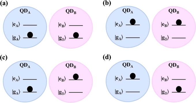
Configuration of the initial states of two spinless electrons of molecular double quantum dot. (a): QD_A is occupied in the ground state |g_A〉 and QD_B is occupied in the ground state |g_B〉, (b): QD_A is occupied in the excited state |e_A〉 and QD_B is occupied in the excited state |e_B〉, (c): QD_A is occupied in the ground state |g_A〉 and QD_B is occupied in the excited state |e_B〉, (d): QD_A is occupied in the excited state |e_A〉 and QD_B is occupied in the ground state |g_B〉.

Mostly, in the study of QDs system for simplification, the coupling of QD with the far-lead is ignored [73]. However, we assume both couplings of each QD to the near-lead and far-lead non-zero with different strengths which are involved in the asymmetric factor definition (Eq. (13)).

According to the definition of asymmetric factor (Eq. (13)), we investigate the entanglement of our proposed quantum dot molecular system in two parts, namely symmetric and asymmetric structures as follows.

4.4. Symmetric structure

The symmetric structure is defined for the equal left and right coupling coefficients of each QD ($T_{AL}=T_{AR}$ and $T_{BL}=T_{BR}$) and also for the same superconducting energy gaps of the left and right reservoirs (${\mathrm{\Delta }}_L={\mathrm{\Delta }}_R$). This situation supplies the minimum magnitude of the asymmetric factor, $\kappa =0$.

For the symmetric structure conditions, the entanglement of QDM system is obtained only for the initial entangled states. These initial states can be considered as the superposition of states in (c) or (d) configurations of Fig. 4 which are known as Bell states. For our system, we assume the initial state of symmetric structure with the highest degree of entanglement as:

$$\rho (0)=\left[\begin{array}{cccc}\hfill 0\hfill & \hfill 0\hfill & \hfill 0\hfill & \hfill 0\hfill \\ \hfill 0\hfill & \hfill 0.5\hfill & \hfill -0.5i\hfill & \hfill 0\hfill \\ \hfill 0\hfill & \hfill 0.5i\hfill & \hfill 0.5\hfill & \hfill 0\hfill \\ \hfill 0\hfill & \hfill 0\hfill & \hfill 0\hfill & \hfill 0\hfill \end{array}\right].$$ (14)

4.5. Asymmetric structure

We introduce the asymmetric structure for the left-right different coupling coefficients with $0<\kappa \le 1$ magnitude and the unequal order parameters of reservoirs, ${\mathrm{\Delta }}_L\ne {\mathrm{\Delta }}_R$. In this group, the ideal asymmetry element is achieved for the maximum amount of asymmetric factor $\kappa \simeq 1$. The situation of ideal asymmetry is available when one of the left or right coupling coefficient is much larger than the other one. To apply the ideal asymmetry properties in physically rational considerations, we assume that each QD is coupled to the near-lead with much larger strength than the far-lead. In other words, we consider ${\mathrm{\Gamma }}_{AL}\gg {\mathrm{\Gamma }}_{AR}$ and ${\mathrm{\Gamma }}_{BR}\gg {\mathrm{\Gamma }}_{BL}$ to provide the most magnitude of asymmetric factor.

It is interesting that the entanglement of our composed systems in asymmetric structure is realized for the initial unentangled states. These states can involve in one of (a) or (b) configurations in Fig. 4. Here, we choose (a) configuration as the initial state for the asymmetric structure which means that both QDs are occupied in their ground states. To investigate this significant situation in the present system, we assume an appropriate separated initial state as:

$$\rho (0)=\left[\begin{array}{cccc}\hfill 1\hfill & \hfill 0\hfill & \hfill 0\hfill & \hfill 0\hfill \\ \hfill 0\hfill & \hfill 0\hfill & \hfill 0\hfill & \hfill 0\hfill \\ \hfill 0\hfill & \hfill 0\hfill & \hfill 0\hfill & \hfill 0\hfill \\ \hfill 0\hfill & \hfill 0\hfill & \hfill 0\hfill & \hfill 0\hfill \end{array}\right].$$ (15)

In the next section, we present the concurrence behavior of the proposed QDM system for both symmetric and asymmetric structures.

5. Results

In this section, we investigate the concurrence behavior of molecular system firstly in response to the bias voltage, secondly by the time evolution in constant voltage and finally through the dynamics for specific superconducting energy gaps.

5.1. Concurrence-voltage characteristics

In this study, concurrence is considered as a function of bias voltage which indirectly depends on the distribution function of reservoirs. According to the Fig. 2, applied asymmetric bias voltage leads to shifting the energy level of the left reservoir with the eV magnitude. Therefore, we can investigate the effect of bias voltage on the concurrence through the concurrence-voltage characteristic (C-V) curves in Fig. 5.

Figure 5.

Concurrence-voltage characteristics for Panel (a): symmetric structure with κ = 0 and Panel (b): asymmetric structure with κ = 0.95; Γ₀ = πN_F|T|².

Fig. 5 is plotted in two panels (a) and (b) for symmetric and asymmetric structures respectively. The solid line curve in this figure demonstrates the concurrence of quantum dot molecule in a normal junction which means that the superconducting energy gap is zero ($\mathrm{\Delta }=0$). However, the curves of dashed and dot-dashed lines show the concurrence of quantum dot molecular system in the Josephson junction with certain superconducting energy gaps. For both panels of Fig. 5, concurrence changes with the step shapes for the normal leads (solid line) and with the delta peaks for the superconducting reservoirs (dot-dashed and dotted lines) in resonant with QDs energy levels.

In panel (a) of Fig. 5, the concurrence for the symmetric structure firstly shows degradation and then it behaves in a saturated way through the increase of voltage. This means that electrons with the entangled initial state in response to the increase of bias voltage can find more opportunities for movement which results in the entanglement degradation. The important point is that although QDM system demonstrates entanglement reduction, it is never unentangled completely with the zero amount. For more bias voltage, the entangled states of electrons can preserve the saturated entanglement with a moderate magnitude.

For panel (b) of Fig. 5 with the initial unentangled states, concurrence demonstrates increasing. Also, for high values of bias voltage, it indicates saturation behavior with the remarkable entanglement amount. This means that electrons with the asymmetric structure through the bias voltage raising can have more possibilities for entanglement. Also, the situation of left-right asymmetric coupling coefficients provides quantum dots to become robustly entangled. Obviously, Fig. 5b shows that for convenient superconducting energy gaps of reservoirs (dot-dashed curve), saturated entanglement can be achieved with the maximum amount.

It is significant that the proposed QDM system can protect saturated entanglement with robust amount for the asymmetric situation.

5.2. Dynamics of concurrence in low bias voltage

Concurrence through the time evolution is shown in Fig. 6 with two panels. Panel (a) which is plotted for the symmetric structure has a minimum asymmetric factor with the value of zero. It occurs when the coupling coefficients of left and right sides are assumed the same ($\kappa =0$). In this situation, the energy gaps of both left and right reservoirs are considered equal to each other ${\mathrm{\Delta }}_L={\mathrm{\Delta }}_R=\mathrm{\Delta }$. The dynamics of entanglement for this condition starts from the initial entangled state and demonstrates degradation by time. After high enough time, it reaches the zero amount which means that electrons of QDM are separated completely. Also, this figure shows that the curves with larger superconducting energy gaps collapse faster.

Figure 6.

Time evolution of concurrence for the constant low bias voltage, Panel (a): the symmetric structure with κ = 0 and Panel (b): the asymmetric structure with κ = 0.95; Γ₀ = πN_F|T|².

In panel (b) of this figure, the asymmetric structure for the QDM system is represented for the large asymmetric factor ($\kappa =0.95$) with the asymmetrical left-right coupling coefficients. Moreover, the superconducting energy gaps of leads are assumed unequal. For this situation, the dynamics of concurrence begins from the initial unentangled state (Eq. (15)) and illustrates increasing. After a long enough time, it shows saturated entanglement. Moreover, the energy gaps of superconducting reservoirs with the higher amounts provide larger entanglement magnitudes. This behavior is such that robust maximum concurrence can be achieved for the convenient situation of the dot-dashed line.

5.3. Dynamics of concurrence for specific superconducting energy gaps

Fig. 7 shows the time evolution of concurrence with regards to the proximity effect of superconducting reservoirs for symmetric and asymmetric situations in panel (a) and panel (b), respectively. In this figure, bias voltages in resonant with energies of quantum dots A and B are influenced by the superconducting proximity effect of the reservoirs. Therefore, they have different concurrence magnitudes for the left and right sides of the resonant points. These resonant points which are $eV-{\epsilon }_A+{\mathrm{\Delta }}_L$ and $eV-{\epsilon }_B+{\mathrm{\Delta }}_R$ are illustrated as peaks with respect to the bias voltage in Fig. 5.

Figure 7.

Dynamics of concurrence for bias voltages in resonant with QD's energy levels, panel (a) for the symmetric structure with Δ_L = Δ_R = Δ and panel (b) for the asymmetric structure. Solid line: left side of the first resonant point, Dashed line: right side of the first resonant point, Dot-dashed line: left side of the second resonant point, Dotted line: right side of the second resonant point and Thick-dashed line: high bias; Γ₀ = πN_F|T|².

In panel (a) for the symmetric structure, the first resonant point ($eV-{\epsilon }_A+{\mathrm{\Delta }}_L\pm 0.01$) has longer elapsed time than the second resonant point ($eV-{\epsilon }_B+{\mathrm{\Delta }}_R\pm 0.01$). In which, the former corresponds to the lower bias voltage. In panel (b) of this figure for the asymmetric situation, the curves of second resonant point ($eV-{\epsilon }_B+{\mathrm{\Delta }}_R\pm 0.01$) indicate larger concurrence amount than the first one ($eV-{\epsilon }_A+{\mathrm{\Delta }}_L\pm 0.01$). For this panel, the latter condition belongs to the lower bias voltage According to the increase of the bias voltage, this behavior of resonant points for both panels reveals that the amount of bias voltage plays more significant role than the other elements in the concurrence time evolution. In addition, for the high bias voltage $eV\gg 0$, the dynamics of system decays in the middle rate of second resonant point curves with decreasing behavior for the symmetric situation in panel (a) and with increasing behavior for the asymmetric situation in panel (b).

The most important difference between panels (a) and (b) originates from their different initial states and also their values of the asymmetric factor for the coupling coefficients which leads to the decrement and increment behavior, respectively. Remarkably, in the asymmetric situation of the system (Fig. 7(b)), the concurrence curves for the proximity effect in both resonant points firstly grow by time and then reach the ultimate magnitude steadily. Moreover, for the second resonant point, concurrence can receive the maximally unit amount through time.

In addition, it is interesting to mention that in spite of the surrounding temperature which usually causes entanglement degradation, there are some situations in which under the effect of environment-assisted, revival entanglement occures [74]. We believe that for the present quantum dot molecular system, investigating the dynamics of entanglement with respect to temperature variations is possible that we plan to do in the future works.

6. Conclusion

In summary, we proposed a procedure to obtain the perfect entanglement for two coupled QDs molecule in a voltage-controlled junction. In this strategy, we focused on the arrangement of different controlling elements to enhance the quantum information characteristics of the system. First, by engineering the reservoirs, we applied superconductors as leads using the significant properties of Josephson junction under the bias voltage control. Second, we utilized the energy couplings of QD-reservoirs asymmetrically. The main advantage of this hybrid quantum system refers to its controllability due to the easy tuning bias voltage and also its coupling coefficients arrangement by manipulating the quantum dot barriers to obtain the required results. In concurrence-voltage characteristics, applying the asymmetric coupling energy conditions can provide a high degree of entanglement while for the symmetric situation, the entanglement shows degradation.

Declarations

Author contribution statement

E. Afsaneh, M. Bagheri Harouni: Conceived and designed the analysis; Analyzed and interpreted the data; Wrote the paper.

Funding statement

This research did not receive any specific grant from funding agencies in the public, commercial, or not-for-profit sectors.

Competing interest statement

The authors declare no conflict of interest.

Additional information

Supplementary content related to this article has been published online at https://doi.org/10.1016/j.heliyon.2020.e04484.

Supplementary material

The following is the Supplementary material related to this article.

Supplementary1.pdf

Diagonalizing the Hamiltonian of superconducting leads.

Supplementary2.pdf

Dynamics of system.

References

- 1.Peres A. Springer Science and Business Media; 2006. Quantum Theory: Concepts and Methods. [Google Scholar]
- 2.Bennett C.H., DiVincenzo D.P., Smolin J.A., Wootters W.K. Phys. Rev. A. 1996;54:3824. doi: 10.1103/physreva.54.3824. [DOI] [PubMed] [Google Scholar]
- 3.Werner R.F. Phys. Rev. A. 1989;40:4277. doi: 10.1103/physreva.40.4277. [DOI] [PubMed] [Google Scholar]
- 4.Alber G., Beth T., Horodecki M., Horodecki P., Horodecki R., Rötteler M., Weinfurter H., Werner R., Zeilinger A. Springer; Berlin Heidelberg: 2003. Quantum Information: An Introduction to Basic Theoretical Concepts and Experiments. [Google Scholar]
- 5.Nielson M.A., Chuang I.L. 2000. Quantum Computation and Quantum Information. [Google Scholar]
- 6.Schliemann J., Cirac J.I., Kuś M., Lewenstein M., Loss D. Phys. Rev. A. 2001;64 [Google Scholar]
- 7.Eckert K., Schliemann J., Bruß D., Lewenstein M. Ann. Phys. 2002;299:88–127. [Google Scholar]
- 8.Zanardi P. Phys. Rev. Lett. 2001;87 doi: 10.1103/PhysRevLett.87.077901. [DOI] [PubMed] [Google Scholar]
- 9.Wiseman H.M., Vaccaro J.A. Phys. Rev. Lett. 2003;91 doi: 10.1103/PhysRevLett.91.097902. [DOI] [PubMed] [Google Scholar]
- 10.Dowling M.R., Doherty A.C., Wiseman H.M. Phys. Rev. A. 2006;73 [Google Scholar]
- 11.Majtey A.P., Bouvrie P.A., Valdés-Hernández A., Plastino A.R. Phys. Rev. A. 2016;93 [Google Scholar]
- 12.Di Tullio M., Gigena N., Rossignoli R. Phys. Rev. A. 2018;97 [Google Scholar]
- 13.Compagno G., Castellini A., Lo Franco R. Philos. Trans. R. Soc. Lond. A. 2018;376 doi: 10.1098/rsta.2017.0317. [DOI] [PubMed] [Google Scholar]
- 14.van Enk S.J. Phys. Rev. A. 2003;67 doi: 10.1103/PhysRevLett.91.017902. [DOI] [PubMed] [Google Scholar]
- 15.Puspus X.M., Villegas K.H., Paraan F.N.C. Phys. Rev. B. 2014;90 [Google Scholar]
- 16.Loss D., DiVincenzo D.P. Phys. Rev. A. 1998;57:120–126. [Google Scholar]
- 17.Hanson R., Kouwenhoven L.P., Petta J.R., Tarucha S., Vandersypen L.M.K. Rev. Mod. Phys. 2007;79:1217–1265. [Google Scholar]
- 18.Buluta I., Ashhab S., Nori F. Rep. Prog. Phys. 2011;74 [Google Scholar]
- 19.Borges H.S., Sanz L., Villas-Bôas J.M., Diniz Neto O.O., Alcalde A.M. Phys. Rev. B. 2012;85 [Google Scholar]
- 20.Carlson C., Dalacu D., Gustin C., Haffouz S., Wu X., Lapointe J., Williams R.L., Poole P.J., Hughes S. Phys. Rev. B. 2019;99 [Google Scholar]
- 21.Bayer M., Hawrylak P., Hinzer K., Fafard S., Korkusinski M., Wasilewski Z.R., Stern O., Forchel A. Science. 2001;291:451–453. doi: 10.1126/science.291.5503.451. [DOI] [PubMed] [Google Scholar]
- 22.Temirov R., Green M.F.B., Friedrich N., Leinen P., Esat T., Chmielniak P., Sarwar S., Rawson J., Kögerler P., Wagner C., Rohlfing M., Tautz F.S. Phys. Rev. Lett. 2018;120 doi: 10.1103/PhysRevLett.120.206801. [DOI] [PubMed] [Google Scholar]
- 23.Oliveira P., Sanz L. Ann. Phys. 2015;356:244–254. [Google Scholar]
- 24.Pérez Daroca D., Roura-Bas P., Aligia A.A. Phys. Rev. B. 2018;97 [Google Scholar]
- 25.Bracker A., Scheibner M., Doty M., Stinaff E., Ponomarev I., Kim J., Whitman L., Reinecke T., Gammon D. Appl. Phys. Lett. 2006;89 doi: 10.1103/PhysRevLett.97.197202. [DOI] [PubMed] [Google Scholar]
- 26.Jennings C., Scheibner M. Phys. Rev. B. 2016;93 [Google Scholar]
- 27.Malz D., Nunnenkamp A. Phys. Rev. B. 2018;97 [Google Scholar]
- 28.Tang G., Zhang L., Wang J. Phys. Rev. B. 2018;97 [Google Scholar]
- 29.Blais A., Girvin S.M., Oliver W.D. Nat. Phys. 2020;16:247. [Google Scholar]
- 30.Clerk A.A., Lehnert K.W., Bertet P., Petta J.R., Nakamura Y. Nat. Phys. 2020;16:257. [Google Scholar]
- 31.Stojanovic V.M. Phys. Rev. Lett. 2020;124 doi: 10.1103/PhysRevLett.124.190504. [DOI] [PubMed] [Google Scholar]
- 32.Lachance-Quirion D., Wolski S.P., Tabuchi Y., Kono Sh., Usami K., Nakamura Y. Science. 2020;367:425. doi: 10.1126/science.aaz9236. [DOI] [PubMed] [Google Scholar]
- 33.Chen Ming-Cheng, Li R., Gan L., Zhu X., Yang G., Lu Chao-Yang, Pan Jian-Wei. Phys. Rev. Lett. 2020;124 doi: 10.1103/PhysRevLett.124.080502. [DOI] [PubMed] [Google Scholar]
- 34.Anagha M., Mohan A., Muruganandan Th., Behera B.K., Panigrahi P.K. Quantum Inf. Process. 2020;19:147. [Google Scholar]
- 35.Mukai H., Sakata K., Devitt S.J., Wang R., Zhou Y., Nakajima Y., Tsai Jaw-Shen. New J. Phys. 2020;22 [Google Scholar]
- 36.Xu Y., Hua Z., Chen T., Pan X., Li X., Han J., Cai W., Ma Y., Wang H., Song Y.P., Xue Zheng-Yuan, Sun L. Phys. Rev. Lett. 2020;124 doi: 10.1103/PhysRevLett.124.230503. [DOI] [PubMed] [Google Scholar]
- 37.Martinis J.M., Nam S., Aumentado J., Urbina C. Phys. Rev. Lett. 2002;89 doi: 10.1103/PhysRevLett.89.117901. [DOI] [PubMed] [Google Scholar]
- 38.Miyanishi K., Matsuzaki Y., Toida H., Kakuyanagi K., Negoro M., Kitagawa M., Saito Sh. Phys. Rev. A. 2020;101 [Google Scholar]
- 39.Yang Y.C., Coppersmith S., Friesen M. npj Quantum Inf. 2019;5:12. [Google Scholar]
- 40.McRae C.R.H., Lake R.E., Long J.L., Bal M., Wu X., Jugdersuren B., Metcalf T.H., Liu X., Pappas D.P. Appl. Phys. Lett. 2020;116 [Google Scholar]
- 41.Stern M., Catelani G., Kubo Y., Grezes C., Bienfait A., Vion D., Esteve D., Bertet P. Phys. Rev. Lett. 2014;113 doi: 10.1103/PhysRevLett.113.123601. [DOI] [PubMed] [Google Scholar]
- 42.Puebla R., Abah O., Paternostro M. Phys. Rev. B. 2020;101 doi: 10.1103/PhysRevLett.124.180401. [DOI] [PubMed] [Google Scholar]
- 43.Xu M., Han Xu, Zou Chang-Ling, Fu W., Xu Y., Zhong Ch., Jiang L., Tang H.X. Phys. Rev. Lett. 2020;124 doi: 10.1103/PhysRevLett.124.033602. [DOI] [PubMed] [Google Scholar]
- 44.Gambetta J., Blais A., Boissonneault M., Houck A.A., Schuster D.I., Girvin S.M. Phys. Rev. A. 2008;77 [Google Scholar]
- 45.Blais A., Gambetta J., Wallraff A., Schuster D.I., Girvin S.M., Devoret M.H., Schoelkopf R.J. Phys. Rev. A. 2007;75 doi: 10.1103/PhysRevLett.99.050501. [DOI] [PubMed] [Google Scholar]
- 46.Santos J.P., Semião F.L. Phys. Rev. A. 2014;89 [Google Scholar]
- 47.Woldeyohannes M., John S. Phys. Rev. A. 1999;60:5046–5068. [Google Scholar]
- 48.Reed M.A., Zhou C., Muller C., Burgin T., Tour J. Science. 1997;278:252–254. [Google Scholar]
- 49.Park H., Park J., Lim A.K., Anderson E.H., Alivisatos A.P., McEuen P.L. Nature. 2000;407:57. doi: 10.1038/35024031. [DOI] [PubMed] [Google Scholar]
- 50.Dadosh T., Gordin Y., Krahne R., Khivrich I., Mahalu D., Frydman V., Sperling J., Yacoby A., Bar-Joseph I. Nature. 2005;436:677. doi: 10.1038/nature03898. [DOI] [PubMed] [Google Scholar]
- 51.Stafford C.A., Wingreen N.S. Phys. Rev. Lett. 1996;76:1916–1919. doi: 10.1103/PhysRevLett.76.1916. [DOI] [PubMed] [Google Scholar]
- 52.Nitzan A., Ratner M.A. Science. 2003;300:1384–1389. doi: 10.1126/science.1081572. [DOI] [PubMed] [Google Scholar]
- 53.Smit R., Noat Y., Untiedt C., Lang N., van Hemert M.V., Van Ruitenbeek J. Nature. 2002;419:906. doi: 10.1038/nature01103. [DOI] [PubMed] [Google Scholar]
- 54.Martin-Rodero A., Yeyati A.L. Adv. Phys. 2011;60:899–958. [Google Scholar]
- 55.Pala M.G., Governale M., Konig J. New J. Phys. 2008;10 [Google Scholar]
- 56.Kosov D.S., Prosen T., Žunkovič B. J. Phys. Condens. Matter. 2013;25 doi: 10.1088/0953-8984/25/7/075702. [DOI] [PubMed] [Google Scholar]
- 57.Pfaller S., Donarini A., Grifoni M. Phys. Rev. B. 2013;87 [Google Scholar]
- 58.Afsaneh E., Yavari H. Few-Body Syst. 2014;55:159–170. [Google Scholar]
- 59.Jovchev A., Anders F.B. Phys. Rev. B. 2013;87 [Google Scholar]
- 60.Khedri A., Meden V., Costi T. Phys. Rev. B. 2017;96 [Google Scholar]
- 61.Nazarov Y.V., Blanter Y.M. Cambridge University Press; 2009. Quantum Transport: Introduction to Nanoscience. [Google Scholar]
- 62.Ekström J., Recher P., Schmidt Th.L. Phys. Rev. B. 2020;101 [Google Scholar]
- 63.De Gennes P. Westview Press; 1999. Superconductivity of Metals and Alloys. [Google Scholar]
- 64.Tinkham M. Courier Corporation; 2004. Introduction to Superconductivity. [Google Scholar]
- 65.Skomski R., Zhou J., Istomin A.Y., Starace A.F., Sellmyer D.J. J. Appl. Phys. 2005;97 [Google Scholar]
- 66.Galve F., Pachon L.A., Zueco D. Phys. Rev. Lett. 2010;105 doi: 10.1103/PhysRevLett.105.180501. [DOI] [PubMed] [Google Scholar]
- 67.Pickett W.E. Rev. Mod. Phys. 1989;61:433. [Google Scholar]
- 68.Mahan G.D. Springer Science and Business Media; 1990. Many-Particle Physics. [Google Scholar]
- 69.Harbola U., Esposito M., Mukamel S. Phys. Rev. B. 2006;74 doi: 10.1103/PhysRevE.76.031132. [DOI] [PubMed] [Google Scholar]
- 70.Hill S., Wootters K. Phys. Rev. Lett. 1997;78:5022. [Google Scholar]
- 71.Wootters W.K. Phys. Rev. Lett. 1998;80:2245. [Google Scholar]
- 72.Rungta P., Bužek V., Caves C.M., Hillery M., Milburn G.J. Phys. Rev. A. 2001;64 [Google Scholar]
- 73.Jiang J.H., Kulkarni M., Segal D., Imry Y. Phys. Rev. B. 2015;92 [Google Scholar]
- 74.Liu F., Zhou Xingxiang, Guo Guang-Can, Zhou Zheng-Wei. Phys. Rev. A. 2020;101 [Google Scholar]
Associated Data
This section collects any data citations, data availability statements, or supplementary materials included in this article.
Supplementary Materials