Computational methods for predicting 3D genomic organization from high-resolution chromosome conformation capture data

Abstract

The advent of high-resolution chromosome conformation capture assays (such as 5C, Hi-C and Pore-C) has allowed for unprecedented sequence-level investigations into the structure–function relationship of the genome. In order to comprehensively understand this relationship, computational tools are required that utilize data generated from these assays to predict 3D genome organization (the 3D genome reconstruction problem). Many computational tools have been developed that answer this need, but a comprehensive comparison of their underlying algorithmic approaches has not been conducted. This manuscript provides a comprehensive review of the existing computational tools (from November 2006 to September 2019, inclusive) that can be used to predict 3D genome organizations from high-resolution chromosome conformation capture data. Overall, existing tools were found to use a relatively small set of algorithms from one or more of the following categories: dimensionality reduction, graph/network theory, maximum likelihood estimation (MLE) and statistical modeling. Solutions in each category are far from maturity, and the breadth and depth of various algorithmic categories have not been fully explored. While the tools for predicting 3D structure for a genomic region or single chromosome are diverse, there is a general lack of algorithmic diversity among computational tools for predicting the complete 3D genome organization from high-resolution chromosome conformation capture data.

Introduction

This manuscript provides a survey of the existing computational tools that can be used for predicting 3D genomic organization from high-resolution chromosome conformation capture data. Relevant biological and computational background is provided in the Background Section. The Problem Formalism Section describes the 3D genome reconstruction problem (3D-GRP) formalism. The section titled Existing Tools for Solving the 3D-GRP provides an overview of existing tools for solving the 3D-GRP. Two of these existing tools (one consensus and one ensemble) are described in more detail in the Exemplar 3D-GRP Tools Section. Similarly, the section titled Predicting 3D Structures for Genomic Regions or Single Chromosomes provides an overview of existing tools for solving the related, but simpler, problem of predicting 3D organization for a single chromosome or genomic region. Exemplar consensus and ensemble tool for solving this simpler problem are discussed in more detail in the Exemplar Regional 3D Prediction Tools Section. Finally, a discussion of the shortcomings of the existing approaches and future research directions can be found in the Future Directions Section.

Background

Like many areas of biology, the relationship between genomic structure and function is closely linked [1]. Alterations in the 3D organization of chromosomes have been demonstrated in a wide variety of nuclear and cellular processes, including DNA translocation [1], differentiation [2], serum response [3], therapeutic response [4] and response to DNA damage [5]. The unique spatial organization of the genome that is seen under these different cellular conditions is hypothesized to be a crucial mechanis driving various nuclear and cellular functions. It has been theorized that this dynamic organization of the genome may be driven by global regulation of gene expression (or vice-versa) [6–10] since 3D genome organization has been shown to facilitate interactions between genes and their regulatory elements [11, 12].

Traditionally, microscopy techniques have been utilized to visualize the spatial organization of chromosomes within the nucleus. While informative, they do not provide sequence-level information about the observed organizations [13]. Therefore, other biological techniques must be used (either in combination or standalone) to allow for the sequence-level inference of 3D genomic organization. Many such biological techniques have been developed to assay the 3D genome organization at various sequence-level resolutions [1, 14–16]. In general, these techniques are able to determine whether a single (or multiple) pair(s) of genomic regions are in close 3D physical proximity. Genomic regions in close proximity are more commonly referred to as ‘interacting’.

The biological techniques used for detecting 3D genomic organization can be broadly classified into the following categories based on the number of genomic regions they assay: one-by-one (used to detect an interaction between a single pair of genomic regions); one-by-all (used to detect all the interactions between one genomic region and the rest of the genome); many-by-many (used to detect interactions between many genomic regions and many other loci, where many is the number of loci on a chip or microarray); many-by-all (used to detect interactions between many genomic regions and the rest of the genome); and all-by-all (used to detect all the interactions occurring between mappable regions of the genome). Table 1 provides the specific names and citations for some of the biological techniques in each of these categories. Briefly, these techniques all follow five general steps (with slight modifications): (i) chemical cross-linking, (ii) fragmentation, (iii) ligation, (iv) reverse cross-linking, and (iv) technique-specific detection. A visual overview of the general workflow for each technique can be found in the review by Denker and de Laat [14]. Additional information regarding the biological background for these techniques can be found in the review recently published by Han et al. [33]. For the purpose of this manuscript, ‘high-resolution chromosome conformation capture’ (HR-3C) will refer to the many-by-many, many-by-all and all-by-all techniques.

Table 1.

Biological techniques that can be used to assay 3D genome organization. Techniques are categorized based on the number of genomic regions they assay

Category	Biological technique(s)
one-by-one	Chromosome conformation capture (3C) [17] and ChiP-loop [18]
one-by-all	Circularized chromosome conformation capture (4C) [19–21]
many-by-many	Chromosome conformation capture carbon copy (5C) [22]
many-by-all	Capture-C [23], Capture Hi-C (CHi-C) [24, 25], HiCap [26] and Target Chromatin Capture (T2C) [27]
all-by-all	ChIA-PET [18], HiChIP [28], Hi-C [29–31], Pore-C [32] and tethered chromatin capture (TCC) [31]

Algorithms for predicting 3D genome structure utilize a set of pairwise interactions and associated frequencies as input. Typically, this data are extracted from the results of a many-by-many, many-by-all or all-by-all (HR-3C) assay. The one-by-one and one-by-all techniques do not generate enough pairwise data points to allow for an accurate prediction of 3D genomic structure on their own. It is possible that the data from a one-by-one or one-by-all assay could be combined with data from an HR-3C assay and used as input to a 3D prediction algorithm, but this is not common practice in the field. The following paragraphs present a brief overview of how a set of pairwise interactions and associated frequencies can be extracted from an HR-3C assay’s raw data (sequencing reads).

In general, HR-3C techniques utilize next-generation sequencing technologies to identify the sequences of interacting regions of the genome. Once these sequencing reads are generated, they are typically processed through a read mapping and filtering pipeline such as HiCUP [34]. Briefly, this process involves quality control, read-splitting and independent read-mapping. Mapping sequence reads to a reference genome results in the generation of a matrix called a whole-genome contact map. A whole-genome contact map is an N × N matrix, where N is the number of genomic ‘bins’ where each bin represents a contiguous sequence of linear DNA [35–37]. In general, the size of the whole-genome contact map (the number of genomic bins) is approximately equal to the total genome size divided by the assay’s experimental resolution. Each cell (A_i,j) of a whole-genome contact map (A) indicates the count of how many times genomic bin i has been found to interact with genomic bin j. These counts are symmetric along the diagonal (i.e. A_i,j = A_j,i) and are often referred to as the frequency of the interaction between A_i and A_j (or interaction frequency).

After the whole-genome contact map is generated, interaction frequencies are normalized to correct for some of the inherent biases resulting from HR-3C experiments. These biases include (but are not limited to) discrepancies in DNA compaction or ‘visibility’ [38], GC content [39, 40] and copy number variation [41]. Various computational methods have been developed to dampen these biases through normalization [40, 42–45]. Most commonly, an iterative correction and eigenvector (ICE) decomposition [38] or Knight–Ruiz normalization [42, 43] is applied resulting in fractional interaction frequencies. ICE decomposition aims to achieve equal visibility across all genomic regions and results in relative interaction frequencies. Knight–Ruiz normalization performs matrix balancing resulting in fractional interaction frequencies where the rows and columns sum to 1. A comprehensive comparison of the normalization methods for HR-3C data has been recently published by Lyu et al. [46]. Downstream analysis of normalized whole-genome contact maps has uncovered unique genome-level patterns including distance-dependent interaction frequencies and more interactions between genomic regions on the same chromosome (cis-chromosomal interactions) than between regions on different chromosomes (trans-chromosomal interactions) [29, 35]. Further computational analysis of whole-genome contact maps has revealed the presence of various ‘hallmarks’ of 3D genome organization. For instance, statistical analysis of whole-genome contact maps has revealed the presence of structural subunits called topologically associating domains (TADs) [47]. TADs are linear regions of DNA where interactions occur more frequently within the domain instead of between domains [47]. Originally, TADs were hypothesized to be structural building blocks for 3D genome organization but it has been determined that they serve no structural importance [48, 49].

Normalized whole-genome contact maps can also be used to infer a 3D structure of the genome (or a single genomic region). The process of predicting a model of the 3D genomic organization from a contact map is known as the 3D-GRP [50] (described in more detail below). Many computational methods have been developed that utilize the data from HR-3C experiments to predict 3D genomic organization. Classically, existing programs have been broadly classified based on the number of genome models the method produces. Ensemble tools generate a collection of structures which represent the different genome organizations that may be present within a population of cells, while consensus tools generate one structure which represents the population-averaged genome organization [35]. This manuscript provides a comprehensive review of the existing tools published from November 2006 (the year 5C was first described [22]) to September 2019 which use data extracted from HR-3C techniques to predict a 3D structure of complete genomes or a genomic region (the sections titled Existing Tools for Solving the 3D-GRP and Predicting 3D Structures for Genomic Regions or Single Chromosomes, respectively). A brief overview of the main chromosome models used by these existing tools is provided in the Problem Formalism section of this manuscript. The subsequent sections assume that the reader has some familiarity with the following concepts: multi-dimensional scaling (MDS) [51, 52], shortest path algorithms [53–56], expectation maximization [57], genetic algorithms [58], gradient descent (or ascent) [59], simulated annealing [60, 61] and Markov chain Monte Carlo (MCMC) sampling [62].

Problem formalism

As mentioned above, the process of predicting a 3D genomic organization from HR-3C data is known as the 3D-GRP [50]. It should be noted that the 3D-GRP has also been referred to as the 3D chromatin structure modeling problem [63] and that these two phrases can be used interchangeably. More formally, the 3D-GRP can be formulated as an optimization problem that tries to optimize the combined distance between multiple pairs of genomic regions. Informally, this is represented as a geometry problem [64] where the genomic bins are encoded as points and the goal is to find each point’s (x, y, z) coordinates such that the pairwise distances between points best capture the corresponding interaction frequencies. It is assumed that, on average, a pair of genomic regions with a small interaction frequency will be further away in 3D space than a pair of genomic regions with a higher interaction frequency [6, 65–72]. This relationship is often modeled through the following inverse function for a given pair of genomic regions (i and j): where dist is the distance between the two genomic regions, A_i,j is the corresponding normalized interaction frequency (a value between 0 and 1) from the whole-genome contact map and α is an exponential factor with a value typically between 0.1 and 3.0 [73]. Most existing methods focus on finding the optimal value (or a set of values) for α and each point’s (x, y, z) coordinates so that the computed distances closely recapitulate the original normalized frequencies from the whole-genome contact map [50]. Formally, the 3D-GRP can be defined in the following way when Euclidean distance is used.

Given a whole-genome contact map A with bins from 1..N, determine α and each point’s (x, y, z) coordinates such tha

(1)

And, the sum

(2)

is minimized and

(3)

In order to predict a 3D organization for a complete genome or genomic region, individual chromosomes need to be modeled as a set of points that can be assigned 3D coordinates. In general, existing methods use one of the following chromosome models. (i) Beads: each individual chromosome is represented as a collection of M beads, where M is the number of genomic bins that constitute the linear extent of a chromosome. (ii) Beads-on-a-String: again, each individual chromosome is represented as a collection of M beads. Unlike the beads model, ‘strings’ of a fixed length are used to connect each pair of adjacent beads. Typically, these represent beads that are linearly adjacent on a chromosome. (iii) Beads-on-a-Spring: this representation is similar to (ii) but beads on an individual chromosome that is connected with ‘springs’ to represent the linear extent of a chromosome. Springs typically have a variable length that is based on attractive and repulsive forces of the connected beads. (iv) Graph/Network: each bin from the whole-genome contact map is represented as a node in a network. Edges between nodes represent interactions from the contact map. Often, edges between bins on the same chromosome that is linearly adjacent are not included. (v) Polymer: each chromosome is represented as a line which is composed of consecutive line segments. Each line segment encodes a genomic bin or a genomic region that is delimited by two endonuclease restriction sites. (vi) Piecewise curve: this is a mathematical formulation where each chromosome is represented as a set of connected 3D curves. Each curve represents an individual genomic bin or region.

Existing tools for solving the 3D-GRP

A comprehensive list of the existing computational tools for predicting 3D genomic organization from HR-3C data is available in Table 2. This table represents the majority of tools in the existing literature at the time of manuscript submission. Additional information regarding how these manuscripts were selected can be found in the Extended Methodology.

Table 2.

Existing computational tools for predicting 3D genome organization from HR-3C data. Tools are categorized as either consensus or ensemble and then listed in alphabetical order. Tools marked with an asterisk (*) did not appear to be actively maintained at the time of manuscript submission. Column headings are as follows: Name, the tool’s name or abbreviated reference (Panel labels from Figure 1 are provided in parentheses); Technique, the general algorithmic strategy employed; CHR model, a description of the chromosome model utilized; Additional data, any additional biological datasets required; A priori Constraints, a descriptor denoting whether a priori information is required and/or assumed; Language, the programing language used to implement the tool; Availability mode, a description of how the tool was deployed; Website, a link to the tool. Abbreviations are as follows: LAD, lamin-associated domains; DamID, DNA adenine methyltransferase identification. IPOPT is a software library used for nonlinear optimization. A dash indicates ‘not applicable’, ‘not available’ or ‘none’, as appropriate

	Name	Technique	CHR model	Additional data	A priori constaints	Language	Availability mode	Website
A: Consensus Methods	Diament and Tuller (Figure 1A) [74]	MDS	Beads-on-a-String	Orthologous relationships	organism-specific (nuclear radius, elasticity between adjacent beads, minimum distance between homolgous CHRs, nucleolous position, CHR 12 position	C++; requires IPOPT	Source Code	http://www.cs.tau.ac.il/∼tamirtul/reconstruction.zip
	Duan et al. (Figure 1B) [6, 65, 75]	MDS	Beads-on-a-String	—	organism-specific (CHR12 position, nucleolous size and position); spatial (1000 nm nucleus, distance between beads (30 or 75 nm for cis-beads, or trans-beads, respectively)	—	—	—
	Kapilevich et al. (Figure 1C) [76]	MDS and Genetic Algorithm	Graph	—	—	Python2	Source Code	https://github.com/skkap/mdsga
	miniMDS (Figure 1D) [77]	MDS with a Divide-and-Conquer Approach	Beads	—	dataset-specific (must have TADs)	Python2 or Python3	Source Code	https://github.com/seqcode/miniMDS
	Segal and Bengtsson (Figure 1E,F) [50]	MDS	Graph	—	—	—	—	—
	Stevens et al. (Figure 1G) [78]	Simulated Annealing	Beads-on-a-String	—	dataset-specific (must be from a single-cell)	Python2 or Python3	Source Code	https://github.com/TheLaueLab/nuc_dynamics
B: Ensemble Methods	Chrom3D (Figure 1H) [79]	Monte Carlo Optimization	Beads-on-a-String	LAD	dataset-specific (must have TADs)	C++	Source Code	https://github.com/Chrom3D/Chrom3D
	Kalhor et al. (Figure 1I) [31]	Simulated Annealing	Beads	—	dataset-specific (must be from a diploid organism, cannot be pre-phased)	—	—	—
	Li et al. (Figure 1J) [80]	Expectation Maximization	Beads	LAD, DamID (only applicable to fruitfly datasets)	organism-specific (nuclear radius, minimum distance between adjacent beads and homolgous CHRs); dataset-specific (must contain TADs)	Python2	Source Code	https://github.com/alberlab/3DGenome_FruitFly
	LorDG* ((Figure 1K) [73]	Gradient Ascent	Beads	—	—	—	—	https://missouri.app.box.com/v/LorDG
	Tjong et al. (Figure 1L) [81]	Expectation Maximization	Beads	—	dataset-specific (must be from a diploid organism, cannot be pre-phased)	—	—	—
C: Consensus or Ensemble Methods	3D-GNOME (Figure 1M) [82, 83]	Simulated Annealing or MDS (low-resolution); Polymer Physics (high-resolution)	Beads-on-a-Spring	—	dataset-specific (must be from organisms that contain CTCF motif)	—	Web Server	http://3dgnome.cent.uw.edu.pl/

In Table 2, the existing tools are categorized based on the number of predicted genome organizations they produce (i.e. ensemble versus consensus). Tools marked with an asterisk (*) did not appear to be actively maintained (DAAM) at the time of manuscript submission. This designation was given if the software presented in the original manuscript(s) could no longer be accessed. Typically, this was due to obsolete or nonfunctional website uniform resource locators. An example of the output produced by each tool can be found in Figure 1. In each case, the images were extracted from the corresponding original publication. Permission was obtained to reprint these images where required¹. All of the existing tools utilize either heuristics or approximations in their solution.

Figure 1.

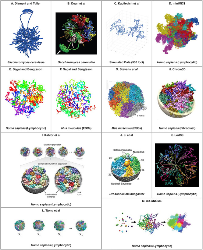
An example of a predicted 3D genome organization from each of the existing consensus (A–G) and ensemble (H–M) tools. Tool name or abbreviated reference can be found at the top of each panel and the organisms (and cell type, when applicable) are listed at the bottom of the panel. The abbreviation ESCs stands for embryonic stem cells. Permission was obtained to reprint these images where required¹.

Five of the seven consensus methods and three of the six ensemble methods that are listed in Table 2 provide access to the source code or a web interface. As mentioned in Table 2, the method developed by Stevens et al. only works with single-cell interaction data, while all other methods accept interaction data from a population of cells. Currently, none of the available, actively maintained ensemble methods are usable for solving the 3D-GRP in the general case. This is because they rely on hypothesized ‘hallmarks’ of genome organization such as TADs, the presence of binding motifs for proteins often found at TAD boundaries (such as CTCF) or require diploid, unphased datasets to make their predictions. This is problematic since these genomic ‘hallmarks’ have been shown to not exist in some organisms such as Arabidopsis thaliana [84, 85]. This could pose a major barrier going forward as investigations into the 3D genomic organization of nonmodel organisms continues.

Exemplar 3D-GRP tools

The following section provides a more detailed discussion of an exemplar consensus and an exemplar ensemble method for solving the 3D-GRP. These methods were chosen since they were the most recent additions to the set of tools presented in Table 2 that have been used by the community to predict 3D genome structure based on real (rather than simulated) HR-3C datasets.

Consensus: miniMDS

miniMDS [77] is a consensus method that combines metric MDS with a divide-and-conquer approach to solve the 3D-GRP. Briefly and in general terms, the local structure of each chromosome is solved and then fitted to a low-resolution global genome prediction. First, a hidden Markov model is used to locally partition each chromosome into a set of subproblems. This hidden Markov model is derived from the TAD-finding algorithm developed by Dixon et al. [47] to identify the local regions of a chromosome where edges of the region preferentially interact with the opposite side of the region. Each subproblem is then converted to a distance matrix based on Equation (4), and metric MDS is used to solve a high-resolution local structure. It should be noted that the zero-distances (typically unmappable genomic regions) are ignored by MDS. This step is then repeated for each complete chromosome at a lower resolution. High-resolution local structures are fitted to these lower resolution chromosome structures using the Kabsch algorithm [86]. Finally, this fitting is repeated at an even lower resolution using the whole dataset to generate a low-resolution global 3D structure. This global structure is then used as the final guide to position the chromosome structures resulting in a completed 3D genome prediction. An example of the output produced by miniMDS can be seen in Figure 1D. miniMDS should be used with caution in organisms where the existence of TADs or TAD-like structures has not been established since the hidden Markov model used for the initial division relies on the presence of TAD-like structures.

(4)

Ensemble: Li et al

The method developed by Li et al. [80] is an ensemble method that incorporates data from lamina-DamID experiments (which are able to detect interactions between the nuclear lamina and genomic regions) with HR-3C data to predict a 3D genomic organization at TAD-level resolution. The data from lamina-DamID experiments allow for the identification of which TAD regions interact with the nuclear envelope (the periphery of the nucleus; abbreviated NE). Briefly, this method uses MLE to find a set of 3D genome structures that have statistically consistent TAD-TAD and TAD-NE interactions. Specifically, this method uses a variant of expectation maximization described by Tjong et al. [81] to optimize this joint probability. It incorporates additional spatial constraints into the optimization based on the known features of the Drosophila melanogaster (fruit fly) genome. These Drosophila-specific constraints are based on microscopy imaging and include the nuclear radius, a maximum distance between chromosome copies, a maximum distance between adjacent TADs, links between heterochromatin regions, links between adjacent TADs and centromere anchoring to the nucleolus. Due to these additional constraints, this method should only be applied to datasets from D. melanogaster and would not be suitable for solving the 3D-GRP in the general case. An example of the output produced by this tool can be seen in Figure 1J. This method could potentially be applied to other organisms with TADs if the required organism-specific spatial constraints are available.

Predicting 3D structures for genomic regions or single chromosomes

There are significantly more tools available that can be used to predict 3D structure of a single genomic region or chromosome from HR-3C data. For the purpose of this manuscript, we will refer to this as 3D regional prediction. The increased number of available tools for 3D regional prediction is likely because it is a much simpler (and often smaller) problem than the 3D-GRP since it does not have to take trans-chromosomal interactions (interactions between genomic regions on different chromosomes) into account. In the majority of cases, it would be computationally infeasible to apply these tools to the 3D-GRP due to their underlying time complexities. It may be possible to overcome this problem by applying a divide-and-conquer approach similar to miniMDS [77]. Table 3 provides a list of the computational techniques that utilize HR-3C data to predict a 3D structure for a given genomic region instead of the whole genome. As described above, tools have been categorized in the following ways: DAAM (*), consensus and/or ensemble. An example of the output produced by each actively maintained consensus and ensemble tool can be found in Figures 2 and 3, respectively. In each case, the images were extracted from the corresponding original publication. Permission was obtained to reprint these images where required^2,3.

Table 3.

Existing computational tools for predicting 3D organization for a genomic region from HR-3C data. Tools are categorized as either consensus or ensemble and then listed in alphabetical order. Tools marked with an asterisk (*) did not appear to be actively maintained at the time of submission. Column headings are as follows: Name, the tool’s name or abbreviated reference (panel labels from Figures 2 and 3 are provided in parentheses); Technique, the general algorithmic strategy employed; CHR model, a description of the chromosome model utilized; Additional data, any additional biological datasets required; A priori constraints, a descriptor denoting whether a priori information is required and/or assumed; Language, the programming language used to implement the tool; Availability mode, a description of how the tool was deployed; Website, a link to the tool’s source code. Abbreviations are as follows: IMP, integrative modeling platform (https://integrativemodeling.org/). A dash indicates ‘not applicable’, ‘not available’ or ‘none’, as appropriate

	Name	Technique	CHR model	Additional data	A priori constraints	Language	Software availability	Website
A: Consensus Methods	AutoChrom3D* [88]	MLE	Beads-on-a-String	—	dataset-specific (must be from a haploid organism or pre-phased)	—	—	http://ibi.hzau.edu.cn/3dmodel/
	BACH (Figure 2A) [70]	MCMC	Beads-on-a-String	—	dataset-specific (must be from a haploid organism or pre-phased)	C++	—	http://www.fas.harvard.edu/∼junliu/BACH/
	Chiariello et al. (Figure 2B) [89]	Polymer Modeling (String & Binders Switch)	Beads-on-a-String	—	dataset-specific (must be from a haploid organism or pre-phased)	—	—	—
	ChromSDE (Figure 2C) [63]	Semi-Definite Programming	Graph	—	dataset-specific (must be from a haploid organism or pre-phased)	—	—	—
	5C3D* [90, 91]	Gradient Descen	Beads (Distributed in a Cube)	—	dataset-specific (must be from a haploid organism or pre-phased)	—	—	http://dostielab.biochem.mcgill.ca/
	HSA* [92]	Simulated Annealing with MCMC	Beads-on-a-String	—	dataset-specific (must be from a haploid organism or pre-phased)	—	—	http://ouyanglab.jax.org/hsa/
	PASTIS (MDS–Figure 2D) [71]	MDS	Beads	—	dataset-specific (must be from a haploid organism or pre-phased)	Python2	Source Code	http://projets.cbio.mines-paristech.fr/∼nvaroquaux/pastis/
	PASTIS (NMDS –Figure 2D) [71]	Non-Metric MDS	Beads	—	dataset-specific (must be from a haploid organism or pre-phased)	Python2	Source Code	http://projets.cbio.mines-paristech.fr/∼nvaroquaux/pastis/
	PASTIS (PM1–Figure 2D) [71]	MLE	Beads	—	dataset-specific (must be from a haploid organism or pre-phased)	Python2	Source Code	http://projets.cbio.mines-paristech.fr/∼nvaroquaux/pastis/
	PASTIS (PM2–Figure 2D) [71]	MLE	Beads	—	dataset-specific (must be from a haploid organism or pre-phased)	Python2	Source Code	http://projets.cbio.mines-paristech.fr/∼nvaroquaux/pastis/
	RPR (Figure 2E) [64]	MDS & Recurrence Plots	Beads	—	dataset-specifc (must be from a single-cell, must be from a haploid organism or pre-phased)	Matlab	Source Code (embedded in a PDF)	https://media.nature.com/original/nature-assets/srep/2016/161011/srep34982/extref/srep34982-s1.pdf
	ShRec3D (Figure 2F) [72, 93]	Shortest Path and MDS	Beads-on-a-Spring	—	organism-specific (nuclear radius), dataset-specific (must be from a haploid organism or pre-phased)	Matlab	Source Code	https://sites.google.com/site/julienmozziconacci/home/softwares
	ShRec3D+ (Figure 2G) [94]	Shortest Path and MDS	Beads-on-a-String	—	dataset-specific (must be from a haploid organism or pre-phased), user-specific (value of for alpha)	—	—	—
	SuperRec (Figure 2H) [37]	Shortest Path and MDS	Beads-on-a-String	—	dataset-specific (must be from a haploid organism or pre-phased)	Python and Linux Executable	Source Code	http://www.cs.cityu.edu.hk/∼shuaicli/SuperRec/
	3DChrom (Figure 2I) [87]	MDS	Beads	—	dataset-specific (must have TADs, must be from a haploid organism or pre-phased)	C++; requires IPOPT	Source Code or Web Server	http://dna.cs.miami.edu/3DChrom/
	tPAM (Figure 2J) [95]	MCMC	Beads	—	dataset-specific (must be from a haploid organism or pre-phased)	—	—	—
	tREX* [96]	Truncated Random Effect Expression Model	Beads	—	dataset-specific (must be from a haploid organism or pre-phased)	—	—	http://www.stat.osu.edu/∼statgen/Software/tRex
	Zhang et al. (Figure 2K) [97]	MCMC	Piecewise Curve (Helical)	—	dataset-specific (must be from a haploid organism or pre-phased)	C++	Source Code	https://rsquared1427.github.io/phm/
B: Ensemble Methods	BACH-MIX (Figure 3A) [70]	MCMC	Beads-on-a-String	—	dataset-specific (must be from a haploid organism or pre-phased)	C++	—	http://www.fas.harvard.edu/∼junliu/BACH/
	Caudai et al. (Figure 3B) [98]	Simulated Annealing and MCMC	Beads	—	dataset-specific (must contain TADs, must be from a haploid organism or pre-phased)	Python2	Source Code	https://bmcbioinformatics.biomedcentral.com/articles/10.1186/s12859-015-0667-0 (AdditionalFile2)
	Chromsome3D (Figure 3C) [99]	Simulated Annealing	Beads-on-a-String	—	dataset-specific (must be from a haploid organism or pre-phased)	Perl	Source Code of Web Server	http://sysbio.rnet.missouri.edu/chromosome3d/
	ChromStruct 4 (Figure 3D) [100]	Simulated Annealing and MCMC	Beads-on-a-String	—	dataset-specific (must be from a haploid organism or pre-phased)	—	—	—
	GEM (Figure 3E) [101]	Manifold Learning & Expectation Maximization	Graph	—	dataset-specific (must be from a haploid organism or pre-phased)	Matlab	Source Code	https://github.com/mlcb-thu/GEM
	Giorgetti et al. (Figure 3F) [102]	Polymer Modeling	Beads-on-a-String	—	dataset-specific (must be from a haploid organism or pre-phased)	—	—	—
	IMP (Figure 3G) [67, 69, 103]	Monte Carlo Optimization	Beads	—	dataset-specific (must be from a haploid organism or pre-phased)	C++ or Python	Binary or Source Code	https://integrativemodeling.org/
	InfMod3DGen (Figure 3H) [104]	Expectation Maximization	Polymer	—	dataset-specific (must be from a haploid organism or pre-phased)	Matlab	Source Code	https://github.com/wangsy11/InfMod3DGen
	ISD (Figure 3I) [105]	Hamiltonian Monte Carlo	Beads	—	dataset-specifc (must be from a single-cell, must be from a haploid or diploid organism)	Python	Source Code	https://github.com/michaelhabeck/isdhic
	MBO (Figure 3J) [106]	Shortest Path and MDS	Beads	—	dataset-specifc (must be from a single-cell, must be from a haploid or diploid organism)	Matlab	Source Code	http://folk.uio.no/jonaspau/mbo/
	MCMC5C (Figure 3K) [68]	MCMC	Piecewise Curve (Linear)	—	organism-specific (homologous chromosomes must make mutally exclusive contacts)	—	—	—
	Meluzzi and Arya (Figure 3L) [107]	Polymer Physics and Adaptive Filter Theory	Beads-on-a-Spring	—	dataset-specific (must be from a haploid organism or pre-phased)	—	—	—
	Nagano et al. (Figure 3M) [108]	Simulated Annealing	Beads-on-a-String	—	dataset-specifc (must be from a single-cell, must be from a haploid organism or pre-phased)	—	—	—
	TADbit (Figure 3O) [103, 109]	IMP	Beads	—	organisms-specific (must have TADs)	Python2	Source Code	https://github.com/3DGenomes/tadbit
	Trieu and Cheng (Figure 3N) [110]	Gradient Descent	Beads	—	organism-specific (only applicable to datasets from H. sapiens), dataset-specific (must be from a haploid organism or pre-phased)	—	—	—

Figure 2.

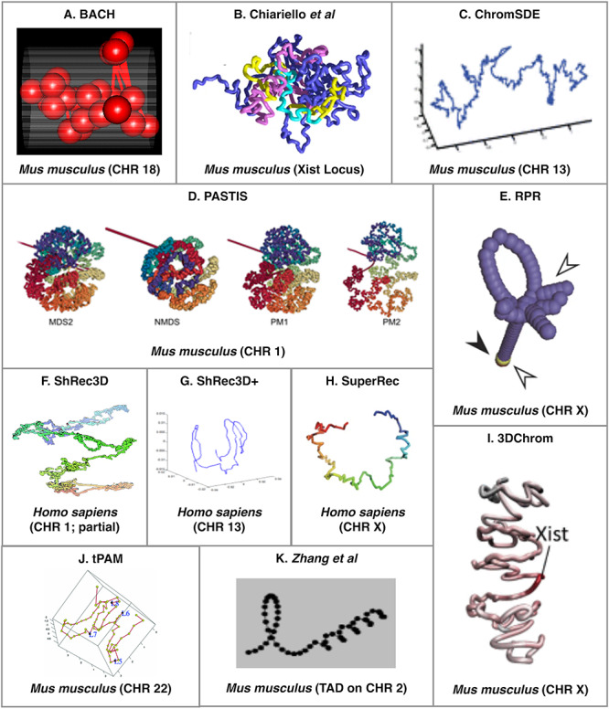
An example of a predicted region organization from each of the existing regional consensus tools. Tool name or abbreviated reference can be found at the top of each panel and the organisms (and specific region, when applicable) are listed at the bottom of the panel. The abbreviation CHR stands for chromosome. Permission was obtained to reprint these images where required².

Figure 3.

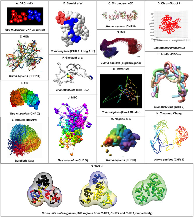
An example of a predicted region organization from each of the existing regional ensemble tools. Tool name or abbreviated reference can be found at the top of each panel and the organisms (and specific region, when applicable) are listed at the bottom of the panel. The abbreviation CHR stands for chromosome. Permission was obtained to reprint these images where required³.

Exemplar regional 3D prediction tools

The following section provides a more detailed discussion of an exemplar consensus and an exemplar ensemble method for predicting the 3D structure of a single genomic region or chromosome. ShRec3D+ was chosen as the exemplar consensus method since it is the most recent version of one of the popular and highly cited tools, ShRec3D [72, 93]. Chromosome3D was chosen as the exemplar ensemble method since it is the most recent addition to set of ensemble tools presented in Table 3 (Chromosome3D) that has been used by the community to predict 3D regional structures (beyond TAD-level resolution) from real population-based HR-3C data (rather than simulated data).

Consensus: ShRec3D+

ShRec3D+ [94] is a consensus method that is based on ShRec3D [72, 93] and ChromSDE [63]. An overview of the approach taken by ShRec3D+ is as follows. First, interactions are converted into a weighted graph where edge weight (which represents the distance between two vertices) is initially calculated with Equation (5), where α is a user-selected value between 0.0 and 2.0. Second, the Floyd–Warshall algorithm is applied to optimize the distances so that the vertices satisfy the triangle inequality. Finally, classical MDS is applied to calculate the (x, y, z) coordinates of each vertex in the graph. An example of the output produced by ShRec3D+ can be seen in Figure 2G⁴. ShRec3D+ does not optimize the value of α like its predecessor ShRec3D. This was done to improve runtime but adds a significant potential for user error in new applications because the user might unintentionally specify an inappropriate value.

(5)

Ensemble: Chromosome3D

Chromsome3D [99] is an ensemble method that models a genomic region as a string of beads. Interaction frequencies are converted to distances based on Equation (6), where K is a scaling constant and α is a tuneable parameter with the suggested values of 11 and 1/3, respectively. Simulated annealing is then used to find the (x, y, z) coordinates for each bead such that the absolute difference between the predicted distances [based on the (x, y, z) coordinates] and initial calculated distances (based on the interaction frequencies) are minimized. This is repeated 20 times to generate an ensemble of potential 3D genomic structures. This set of structures is ranked using Spearman’s rank correlation coefficient to determine which predicted structures best represent the initially distances calculated based on the interaction frequencies. An example of the output produced by Chromosome3D can be seen in Figure 3C. Chromsome3D has been shown to outperform ShRec3D when the input data set is noisy [99], which is a characteristic of HR-3C datasets.

(6)

Future directions

There is a lack of algorithmically diverse solutions to the 3D-GRP that could be applied to a wide-variety of organisms (we refer to this as generalizable for this manuscript). Five of the six consensus methods use an MDS as a part of their approach for solving the 3D-GRP. MDS presents many potential issues which are described in the section titled Increasing Algorithmic Diversity. The remaining method by Stevens et al. can only be used with single-cell HR-3C data. Additionally, none of the available ensemble methods are usable for solving the 3D-GRP in the general case. Only two of the five ensemble methods provide source code and are actively maintained. These two methods also require additional biological datasets (DamID and/or LAD) for 3D genome prediction. These types of datasets are not commonly gathered with HR-3C assays; therefore, these solutions are not applicable in the general case. Finally, the web application 3D-GNOME only works with the precomputed HR-3C datasets hosted on the website. As investigations into the 3D genome organization continue, it is possible that the existing tools cannot be utilized for applications in organisms with larger, more complicated genomes (when compared to Homo sapiens). The reasons and potential solutions are described in the subsections below.

Computational limitations

As mentioned previously, the current formulation of the 3D-GRP is a combinatorial optimization problem. Combinatorial optimization problems are known to be demanding in terms of computational resources such as memory. This is potentially problematic because it adds an upper bound on the number of genomic bins that can be input into existing tools based on available computational resources. This could render certain 3D-GRP solutions impractical for generating high-resolution predictions and/or predictions from organisms with genomes larger than H. sapiens. For instance, these computational limitations cause polymer models to have a genome size and/or resolution limit (i.e. number of ‘beads’). For these polymer modeling-based solutions, the current upper bound on the number of genomic regions that can be predicted has been reported to be 10 000 [111]. The majority of the existing tools have an O(N³) time complexity since they rely on MDS and/or the Floyd–Warshall algorithm. As the resolution of GR-3C data increases so does the value for N. This will necessitate investigations into more efficient approaches. Fortunately, combinatorial optimization problems have been extensively studied in computer science and many of the existing solutions for solving these types of problems could be leveraged in 3D-GRP solutions. Existing tools such as miniMDS have utilized a divide-and-conquer approach to overcome the computational limitations [77]. It is expected that approaches like this (as well as others that take advantage of parallelism or distributed algorithms) will become more common as advances in HR-3C assays continue to allow researchers to obtain finer genomic resolutions. Future research should focus on establishing solutions that are more computationally efficient and/or take advantage of parallel or distributed algorithms to overcome the current computational limitations.

Increasing algorithmic diversity

Algorithms for solving the 3D-GRP are far from maturity [97]. While there is some algorithmic diversity in the set of existing tools, the full breadth and depth of solutions in each category have yet to be explored. As mentioned above, five of the six consensus methods use an MDS as a part of their approach for solving the 3D-GRP. Many issues have been noted pertaining to the use of MDS as a part of solutions to the 3D-GRP. For instance, because HR-3C assays represent a heterogeneous population of genome organizations, there is often not a single unique solution. Therefore, the distances calculated by MDS often conflict and cannot be accurately or completely calculated [99]. Furthermore, it is known that standard MDS techniques are inaccurate for sparse high-resolution data [77]. t-Stochastic neighborhood embedding has been shown to be more accurate than MDS for datasets with these characteristics [112–115] and is a promising technique for new 3D-GRP solutions.

All of the existing methods utilize Euclidean distances in their solutions to the 3D-GRP, but the utility of other distance functions [such as relative Sorensen distances, Canberra distances and cosine (similarity) distances] could and should be investigated going forward to increase the accuracy of predicted models. This is especially pertinent in the case of solutions to the 3D-GRP since it is known that Euclidean distances are often not suitable for sparse, high-dimensional datasets [116] which is the case with many whole-genome contact maps. Finally, most of the existing tools model the chromosome as a set of beads or beads-on-a-string/spring. While this seems like a natural representation, the utility of other chromosome models should be investigated.

In general, there is a lack of algorithmic diversity in the existing set of tools for solving the 3D-GRP. Figure 4 provides a visual depiction of the different algorithmic strategies employed by 3D-GRP solutions (purple boxes), 3D regional prediction solutions (orange boxes) and both (green boxes). Additionally, we highlight a few algorithmic strategies that, to the best of our knowledge, have not yet been utilized for predicting 3D structures of the genome or genetic region (gray boxes). In our opinion, these represent promising areas of exploration for new tool development, but there are many other algorithms and algorithm types well-suited for combinatorial optimization problems that could also be investigated. While the community has made great strides in developing solutions to the 3D-GRP, a lot of work remains to be done as investigations into the 3D genome organization of nonmodel organisms begins.

Figure 4.

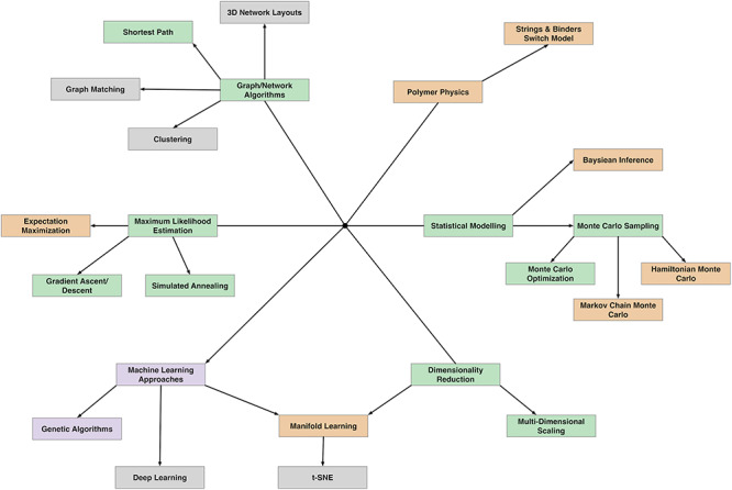
An overview of the algorithmic techniques used by existing tools for solving the 3D-GRP (purple boxes), 3D regional prediction (orange boxes), and both (green boxes). A small selection of unexplored algorithmic strategies is indicated with gray boxes. Lines originate at a black dot and represent the hierarchical relationship between each algorithmic approach (more general to more specific).

Applications to other organisms

An increase in algorithmic diversity is necessary to facilitate 3D genome analysis in nonmodel organisms. As mentioned previously, many methods rely on the presence of previously proposed ‘hallmarks’ of genomic organization such as TADs for prediction. This is troubling since the presence of these ‘hallmarks’ has not been verified in a wide variety of organisms. For instance, recently, it was found that TADs are not present in certain plant species such as A. thaliana [85] and are, therefore, not a conserved hallmark of genome organization. Methods such as miniMDS that rely on TADs or TAD-like structures for efficient computation would not be applicable to organisms such as A. thaliana.

Many of the existing tools have only been utilized with data generated from standard model organisms such as Saccharomyces cerevisiae, Mus musculus or H. sapiens. Table 4 presents an overview of the datasources that have been used by existing tools for solving the 3D-GRP. They are separated with black outlines into the following groups based on their origin: simulated data, parasite, virus, bacteria, yeast, insect, worm, fish, chicken, mice, primate, human and plant. Data sources used in the original manuscript are represented with a gray box. Applications of the tool were determined by reviewing all of the original publications citing articles. The exact number of articles reviewed for each tool is provided in the second column of Table 4. Valid applications of a tool in a different organism and/or dataset than the original paper are indicated with purple (successful) or orange (unsuccessful) boxes. There are many organisms that have Hi-C data available, but 3D genomic predictions have not been performed with any of it (Table 4; white boxes). Interestingly, at the time of publication, there were over 3200 Hi-C datasets deposited in the Gene Expression Omnibus dataset, but complete 3D genome prediction has only been applied to less than 10 unique datasets. This provides an interesting area of future exploration and application in the 3D genomics community.

Table 4.

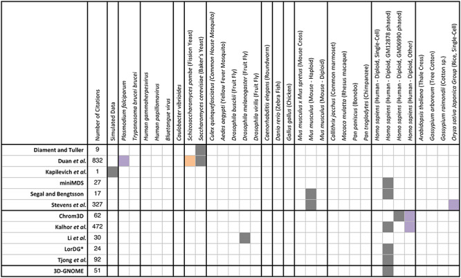
An overview of the data sources that have been used by existing tools for solving the 3D-GRP. Tool name is provided in the first column and follows the same ordering presented in Table 2. The number of citations that were examined is given in column 2. Data sources are listed in the first row and have been separated (black outlines) into the following groups based on their origin: simulated data, parasite, virus, bacteria, yeast, insect, worm, fish, chicken, mice, primate, human and plant. Gray boxes represent the datasource that was used in the original manuscript. Applications of the tool in other organisms are indicated with purple (successful) or orange (unsuccessful) boxes. Datasets that have not been applied to a tool are indicated with a white box.

None of the existing tools have been applied to organisms with a ploidy greater than 2. As such, it is not clear whether these tools can be effectively utilized for predicting 3D genome structure in organisms with higher ploidies such as Triticum aestivum (bread wheat; hexaploid) [117]. Additionally, many of the 3D regional tools do not effectively deal with datasets from polyploid organisms and, therefore, could not be applied to polyploid datasets (or extended to solve the 3D-GRP irregardless of computational complexity). This can be seen when looking at the applications presented in the original manuscripts of the regional tools where most chose to use either a haploid organism, prephased data or a genomic region from the X chromosome of male cells. How to effectively deconvolute interaction signals from distinct chromosome copies (the ploidy problem) still remains a large, unanswered question in the field. While it may be possible to address this problem during read mapping and/or preprocessing steps, solutions built-in to 3D-GRP tools should also be investigated.

Conclusion

There has been a great deal of success predicting 3D genome organizations from HR-3C data originating from model organisms such as S. cerevisiae and H. sapiens.

Addressing the challenges outlined in the Future Directions Section above will be crucial as the field continues to evolve and be extended to nonmodel organisms (especially ones with larger, nonstandard genomes). The set of existing tools for solving the 3D-GRP is far from mature and cannot be applied to analyze 3D genome organization across various species. A tool that can be used to predict 3D genome structure across organisms is urgently needed. Many of the existing solution approaches in computer science for overcoming the difficulties associated with optimization problems such as the 3D-GRP have not yet been explored. These types of solutions are likely to be an area of major development in the coming years within the 3D genome community. While a great deal of foundational work has been done, there is a clear lack of generalizable, algorithmically diverse computational tools for predicting the complete 3D genome organization from HR-3C data.

Key points

• Many computational solutions exist for predicting 3D genome organizations in a select few model organisms.

• These existing tools cannot necessarily be applied to nonmodel organisms due to inherent constraints imposed by the underlying techniques.

• New tools are required to facilitate 3D genome organization studies in nonmodel organisms.

• There are many promising algorithmic areas that have not yet been applied to the 3D-GRP.

• There are many existing Hi-C datasets that have not been used to predict 3D genomic organization with existing tools.

Appendix

• Permission to reprint the images in Figure 1.

  • Figure 1G from Diament and Tuller [74]: Creative Commons Attribution (CC BY) license.

  • A portion of Figure 5 from Duan et al. [65]:

    • License number: 4751560452148; issued on 17 January 2020

  • A portion of Figure 4 from Kapilevich et al. [76]:

    • License number: 4703250178326; issued on 6 November 2019

  • Figure 10 from miniMDS [77]: Creative Commons Attribution-NonCommercial (CC BY-NC 4.0) license.

  • Figures 1 and 2 from Segal and Bengtsson [50]: Creative Commons Attribution (CC BY) license.

  • A portion of Figure 1 from Stevens et al. [78]:

    • License number: 4751560316055; issued on 17 January 2020

  • Figure 3A from Chrom3D: License number: 4811001157261; issued on 16 April 2020

  • Figure 5D from Kalhor et al. [31]:

    • License number: 4703251132971; issued on 6 November 2019

  • A portion of Figure 1C from Li et al. [80]: Creative Commons Attribution (CC BY) license.

  • Figure 10 from LorDG [73]: Creative Commons Attribution-NonCommercial (CC BY-NC 4.0) license.

  • A portion of Figure 1A Tjong et al. [81]: Permission obtained from PNAS via e-mail correspondence on 1 April 2020.

  • Figure 1D from 3D-GNOME [83]: Creative Commons Attribution-NonCommercial (CC BY- NC 4.0) license.

• Permission to reprint the images in Figure 2.

  • Figure 1D from BACH [70]: Creative Commons Attribution (CC BY) license.

  • Figure 5C from Chiariello et al. [89]: Creative Commons Attribution 4.0 International (CC BY 4.0) license.

  • Figure 8 from ChromSDE [63]:

    • License number: 4810860519745; issued on 16 April 2020

  • Figure 3D from PASTIS [71]: Creative Commons Attribution-NonCommercial (CC BY-NC 4.0) license.

  • A portion of Figure 4C from RPR [64]: Creative Commons Attribution (CC BY) license.

  • Figure 3D from ShRec3D [72]:

    • License number: 4751560134989; issued on 17 January 2020

  • A portion of Figure 6B from ShRec3D+ [94]:

    • License number: 4703250567885; issued on 6 November 2019

  • A portion of Figure 8 from SuperRec [37]: Creative Commons Attribution 4.0 International (CC BY 4.0) license.

  • Figure 7A from 3DChrom [87]:

    • License number: 4757200895857; issued on 27 January 2020

  • Figure 5 from tPAM [95]:

    • License number: 4751551505582; issued on 17 January 2020

  • Figure 5B from Zhang et al. [97]:

    • License number: 4757201185227; issued on 27 January 2020

• Permission to reprint the images in Figure 3.

  • Figure 2C from BACH-MIX [70]: Creative Commons Attribution (CC BY) license.

  • A portion of Figure 4 from Caudai et al. [98]: Creative Commons Attribution (CC BY) license.

  • A portion of Figure 4 from Chromsome3D [99]: Creative Commons Attribution 4.0 International (CC BY 4.0) license.

  • A portion of Figure 9 from ChromStruct 4 [100]:

    • License number: 4757201469502; issued on 27 January 2020

  • A portion of Figure 3A from GEM [101]: Creative Commons Attribution-NonCommercial (CC BY-NC 4.0) license.

  • A portion of Figure 6A from Giorgetti et al. [102]:

    • License number: 4751550455329; issued on 17 January 2020.

  • Figure 3B from IMP [67]:

    • License number: 4751550598254; issued on 17 January 2020

  • Figure 6C from InfMod3DGen [104]: Creative Commons Attribution (CC BY) license.

  • A portion of Figure 4A from ISD [105]: Creative Commons Attribution (CC BY) license.

  • Figure 5D from MBO [106]: Creative Commons Attribution (CC BY) license.

  • Figure 7A from MCMC5C [68]: Creative Commons Attribution (CC BY) license.

  • A portion of Figure 9B from Meluzzi and Arya [107]: Creative Commons Attribution-NonCommercial (CC BY-NC 4.0) license.

  • A portion of Figure 3C from Nagano et al. [108]:

    • License number: 4751551203420; issued on 17 January 2020

  • A portion of Figure 4A from TADbit [109]: Creative Commons Attribution (CC BY) license.

  • Figure 11A from Trieu and Cheng [110]: Creative Commons Attribution (CC BY) license.

Kimberly MacKay is a Ph.D. candidate in the Department of Computer Science, University of Saskatchewan.

Anthony Kusalik is a Professor in the Department of Computer Science at the University of Saskatchewan. He also is also the Director of the Bioinformatics Program at the University of Saskatchewan.

Funding

This work was supported by the Natural Sciences and Engineering Research Council of Canada [RGPIN 37207 to AK, Vanier Canada Graduate Scholarship to KM].

References

- 1. Rasim Barutcu A, Fritz AJ, Zaidi SK, et al. C-ing the genome: a compendium of chromosome conformation capture methods to study higher-order chromatin organization. J Cell Physiol 2016;231(1):31–35. [DOI] [PMC free article] [PubMed] [Google Scholar]
- 2. Kuroda M, Tanabe H, Yoshida K, et al. Alteration of chromosome positioning during adipocyte differentiation. J Cell Sci 2004;117:5897–5903. [DOI] [PubMed] [Google Scholar]
- 3. Mehta IS, Amira M, Harvey AJ, et al. Rapid chromosome territory relocation by nuclear motor activity in response to serum removal in primary human fibroblasts. Genome Biol 2010;11(1):R5. [DOI] [PMC free article] [PubMed] [Google Scholar]
- 4. Mehta IS, Eskiw CH, Arican HD, et al. Farne- syltransferase inhibitor treatment restores chromosome territory positions and active chromosome dynamics in Hutchinson-Gilford progeria syndrome cells. Genome Biol 2011;12(8):R74. [DOI] [PMC free article] [PubMed] [Google Scholar]
- 5. Mehta IS, Kulashreshtha M, Chakraborty S, et al. Chromosome territories reposition during DNA damage-repair re-sponse. Genome Biol 2013;14(12):R135. [DOI] [PMC free article] [PubMed] [Google Scholar]
- 6. Ay F, Bunnik EM, Varoquaux N, et al. Three-dimensional modeling of the P. falciparum genome during the erythrocytic cycle re-veals a strong connection between genome architecture and gene expression. Genome Res 2014;24:974–988. [DOI] [PMC free article] [PubMed] [Google Scholar]
- 7. Dekker J. Regulation of gene expression through chromatin interaction networks. Blood Cells Mol Dis 2007;38(2):135. [Google Scholar]
- 8. Chakalova L, Debrand E, Mitchell JA, et al. Replication and transcription: shaping the landscape of the genome. Nat Rev Genet 2005;6(9):669–677. [DOI] [PubMed] [Google Scholar]
- 9. Li Y, Hu M, Shen Y. Gene regulation in the 3d genome. Hum Mol Genet 2018;R2:R228–R233. [DOI] [PMC free article] [PubMed] [Google Scholar]
- 10. Cook PR, Marenduzzo D. Transcription-driven genome organization: a model for chromosome structure and the regulation of gene expression tested through simulations. Nucleic Acids Res 2018;46(19):9896–9906. [DOI] [PMC free article] [PubMed] [Google Scholar]
- 11. Won H, Torre-Ubieta L, Stein JL, et al. Chromosome conformation elucidates regulatory relationships in developing human brain. Nature 2016;538(7626):523–527. [DOI] [PMC free article] [PubMed] [Google Scholar]
- 12. Taberlay PC, Achinger-Kawecka J, Lun ATL, et al. Three-dimensional disorganisation of the cancer genome occurs coincident with long range genetic and epigenetic alterations. Genome Res 2016;26(6):719–731. [DOI] [PMC free article] [PubMed] [Google Scholar]
- 13. Dong Q, Li N, Li X, et al. Genome-wide hi-C analysis reveals extensive hierarchical chromatin interactions in rice. Plant J 2018;94(6):1141–1156. [DOI] [PubMed] [Google Scholar]
- 14. Denker A, Laat W. The second decade of 3C technologies: detailed insights into nuclear organization. Genes Dev 2016;30(12):1357–1382. [DOI] [PMC free article] [PubMed] [Google Scholar]
- 15. Wit E, Laat W. A decade of 3C technologies: insights into nuclear organization. Genes Dev 2017;26:11–24. [DOI] [PMC free article] [PubMed] [Google Scholar]
- 16. Sati S, Cavalli G. Chromosome conformation capture technologies and their impact in understanding genome function. Chromosoma 2017;126(1):33–44. [DOI] [PubMed] [Google Scholar]
- 17. Dekker J, Rippe K, Dekker M, Kleckner N. Capturing chromosome conformation. Science 2002;295(5558):1306–1311. [DOI] [PubMed] [Google Scholar]
- 18. Fullwood MJ, Ruan Y. ChIP-based methods for the identification of long-range chromatin interactions. J Cell Biochem 2009;107(1):30–39. [DOI] [PMC free article] [PubMed] [Google Scholar]
- 19. Würtele H, Chartrand P. Genome-wide scanning of HoxB1-associated loci in mouse ES cells using an open-ended chromosome conformation capture methodology. Chromosome Res 2006;14(5):477–495. [DOI] [PubMed] [Google Scholar]
- 20. Zhao Z, Tavoosidana G, Sjölinder M, et al. Circular chromosome conformation capture (4C) uncovers extensive networks of epigenetically regulated intra- and interchromosomal interactions. Nat Genet 2006;38:1341–1347. [DOI] [PubMed] [Google Scholar]
- 21. Simonis M, Klous P, Splinter E, et al. Nuclear organization of active and inactive chromatin domains uncovered by chromosome conformation capture-on-chip (4C). Nat Genet 2006;38(11):1348–1354. [DOI] [PubMed] [Google Scholar]
- 22. Dostie J, Richmond TA, Arnaout RA, et al. Chromosome conformation capture carbon copy (5C): a massively parallel solution for mapping interactions between genomic elements. Genome Res 2006;16(10):1299–1309. [DOI] [PMC free article] [PubMed] [Google Scholar]
- 23. Hughes JR, Roberts N, McGowan S, et al. Analysis of hundreds of cis-regulatory landscapes at high resolution in a single, high-throughput experiment. Nat Genet 2014;46(2):205–212. [DOI] [PubMed] [Google Scholar]
- 24. Dryden NH, Broome LR, Dudbridge F, et al. Unbiased analysis of potential targets of breast cancer susceptibility loci by capture hi-C. Genome Res 2014;24(11):1854–1868. [DOI] [PMC free article] [PubMed] [Google Scholar]
- 25. Jäger R, Migliorini G, Henrion M, et al. Capture hi-C identifies the chromatin interactome of colorectal cancer risk loci. Nat Commun 2015;6:6178. [DOI] [PMC free article] [PubMed] [Google Scholar]
- 26. Sahlén P, Abdullayev I, Ramsköld D, et al. Genome-wide mapping of promoter-anchored interactions with close to single-enhancer resolution. Genome Biol 2015;16:156. [DOI] [PMC free article] [PubMed] [Google Scholar]
- 27. Kolovos P, Werken HJG, Kepper N, et al. Targeted chromatin capture (T2C): a novel high resolution high throughput method to detect genomic interactions and regulatory elements: a novel high resolution high through-put method to detect genomic interactions and regulatory elements. Epigenetics Chromatin 2014;7:10. [DOI] [PMC free article] [PubMed] [Google Scholar]
- 28. Mumbach MR, Rubin AJ, Flynn RA, et al. HiChIP: efficient and sensitive analysis of protein-directed genome architecture. Nat Methods 2016;13:919–922. [DOI] [PMC free article] [PubMed] [Google Scholar]
- 29. Lieberman-Aiden E, Berkum NL, Williams L, et al. Comprehensive mapping of long range interactions reveals folding principles of the human genome. Science 2009;326(5950):289–293. [DOI] [PMC free article] [PubMed] [Google Scholar]
- 30. Belton J-M, McCord RP, Gibcus JH, et al. Hi–C: a comprehensive technique to capture the conformation of genomes. Methods 2012;58:268–276. [DOI] [PMC free article] [PubMed] [Google Scholar]
- 31. Kalhor R, Tjong H, Jayathilaka N, et al. Genome architectures revealed by tethered chromosome conformation capture and population- based modeling. Nat Biotechnol 2012;30(1):90–98. [DOI] [PMC free article] [PubMed] [Google Scholar]
- 32. Imielinski lab (New York Genome Center) collaboration Pore-C: using nanopore reads to delineate long-range interactions between genomic loci in the human genome. Technical report, Oxford Nanoproe Technologies, (Poster), 2018. https://nanoporetech.com/resource-centre/pore-c-using-nanopore-reads-delineate-long-range-interactions-between-genomic-locikeys=MinION
- 33. Han J, Zhang Z, Wang K. 3C and 3C-based techniques: the powerful tools for spatial genome organization deciphering. Mol Cytogenet 2018;11:21. [DOI] [PMC free article] [PubMed] [Google Scholar]
- 34. Wingett S, Ewels P, Furlan-Magaril M, et al. HiCUP: pipeline for mapping and processing hi-C data. F1000Research 2015;4:1310. [DOI] [PMC free article] [PubMed] [Google Scholar]
- 35. Lajoie BR, Dekker J, Kaplan N. The hitchhiker’s guide to hi-C analysis: practical guidelines. Methods 2015;72:65–75. [DOI] [PMC free article] [PubMed] [Google Scholar]
- 36. MacKay K, Kusalik A, Eskiw CH. GrapHi-C: graph-based visualization of hi-C datasets. BMC Res Notes 2018;11(1):418. doi: 10.1186/s13104-018-3507-2. [DOI] [PMC free article] [PubMed] [Google Scholar]
- 37. Zhang Y, Liu W, Yu L, et al. Large-scale 3D chromatin reconstruction from chromosomal contacts. BMC Genomics 2019;20(Suppl 2):186. [DOI] [PMC free article] [PubMed] [Google Scholar]
- 38. Imakaev M, Fudenberg G, McCord RP, et al. Iterative correction of hi-C data reveals hallmarks of chromosome organization. Nat Methods 2012;9(10):999–1003. [DOI] [PMC free article] [PubMed] [Google Scholar]
- 39. Yaffe E, Tanay A. Probabilistic modeling of hi-C contact maps eliminates systematic biases to characterize global chromosomal architecture. Nat Genet 2011;43:1059–1065. [DOI] [PubMed] [Google Scholar]
- 40. Hu M, Deng K, Selvaraj S, et al. HiCNorm: removing biases in hi-C data via Poisson regression. Bioinformatics 2012;28(23):3131–3133. [DOI] [PMC free article] [PubMed] [Google Scholar]
- 41. Servant N, Varoquaux N, Heard E, et al. Effective normalization for copy number variation in hi-C data. BMC Bioinformatics 2018;19:313. [DOI] [PMC free article] [PubMed] [Google Scholar]
- 42. Knight PA, Ruiz D. A fast algorithm for matrix balancing. J Num Anal 2012;33(3):1029–1047. [Google Scholar]
- 43. Li W, Gong K, Li Q, et al. Hi-corrector: a fast, scalable and memory-efficient package for normalizing large-scale hi-C data. Bioinformatics 2015;31(6):960–962. [DOI] [PMC free article] [PubMed] [Google Scholar]
- 44. Cournac A, Marie-Nelly H, Marbouty M, et al. Normalization of a chromosomal contact map. BMC Genomics 2012;13:436. [DOI] [PMC free article] [PubMed] [Google Scholar]
- 45. Stansfield JC, Cresswell KG, Vladimirov VI, Dozmorov MG. HiCcompare: an R-package for joint normalization and comparison of hi-C datasets. BMC Bioinformatics 2018;19(1):279. [DOI] [PMC free article] [PubMed] [Google Scholar]
- 46. Lyu H, Liu E, Zhifang W. Comparison of normalization methods for hi-C data. Biotechniques 2020;68(2):56–64. [DOI] [PubMed] [Google Scholar]
- 47. Dixon JR, Selvaraj S, Yue F, et al. Topological domains in mammalian genomes identified by analysis of chromatin interactions. Nature 2012;485(7398):376–380. [DOI] [PMC free article] [PubMed] [Google Scholar]
- 48. Zhan Y, Mariani L, Barozzi I, et al. Reciprocal insulation analysis of hi-c data shows that TADs represent a functionally but not structurally privileged scale in the hierarchical folding of chromosomes. Genome Res 2017;27(3):479–490. [DOI] [PMC free article] [PubMed] [Google Scholar]
- 49. Wit E. TADs as the caller calls them. J Mol Biol 2020; 432(3):638–642. [DOI] [PubMed] [Google Scholar]
- 50. Segal MR, Bengtsson HL. Reconstruction of 3D genome architecture via a two-stage algorithm. BMC Bioinformatics 2015;16:373. [DOI] [PMC free article] [PubMed] [Google Scholar]
- 51. Kruskal JB. Multidimensional scaling by optimizing goodness of fit to a non-metric hypothesis. Psychometrika 1964;29(1):1–27. [Google Scholar]
- 52. Kruskal JB. Nonmetric multidimensional scaling: a numerical method. Psychometrika 1964;29(2):115–129. [Google Scholar]
- 53. Dijkstra EW. A note on two problems in connexion with graphs. Numerische Mathematik 1959;1(1):269–271. [Google Scholar]
- 54. Floyd RW. Algorithm 97: shortest path. Commun ACM 1962;5(6):345. [Google Scholar]
- 55. Warshall S. A theorem on boolean matrices. J ACM 1962;9(1):11–12. [Google Scholar]
- 56. Johnson DB. Efficient algorithms for shortest paths in sparse networks. J ACM 1977;24(1):1–13. [Google Scholar]
- 57. Dempster AP, Laird NM, Rubin DB. Maximum likelihood from incomplete data via the EM algorithm. J Royal Stat Soc, Series B 1977;39(1):1–38. [Google Scholar]
- 58. Srinivas M, Patnaik LM. Genetic algorithms: a survey. Computer 1994;27(6):17–26. [Google Scholar]
- 59. Barzilai J, Borwein JM. Two-point step size gradient methods. IMA J Numerical Anal 1988;8(1):141–148. [Google Scholar]
- 60. Kirkpatrick S, Gelatt CD, Vecchi MP. Optimization by simulated annealing. Science 1983;220(4598):671–680. [DOI] [PubMed] [Google Scholar]
- 61. Szu H, Hartley R. Fast simulated annealing. Phys Lett A 1987;122(3–4):157–162. [Google Scholar]
- 62. Hastings WK. Monte Carlo sampling methods using Markov chains and their applications. Biometrika 1970;57(1):97–109. [Google Scholar]
- 63. Zhang Z, Li G, Toh K-C, et al. 3D chromosome modeling with semi-definite programming and hi-C data. J Comput Biol 2013;20(11):831–846. [DOI] [PubMed] [Google Scholar]
- 64. Hirata Y, Oda A, Ohta K, et al. Three-dimensional reconstruction of single-cell chromosome structure using recurrence plots. Sci Rep 2016;6:34982. [DOI] [PMC free article] [PubMed] [Google Scholar]
- 65. Duan Z, Andronescu M, Schutz K, et al. A three-dimensional model of the yeast genome. Nature 2010;465:363–367. [DOI] [PMC free article] [PubMed] [Google Scholar]
- 66. Fraser James, Rousseau Mathieu, Blanchette Mathieu, et al. Computing chromosome conformation. Totowa, NJ: Humana Press, 2010, 251–68. ISBN 978-1-60761-854-6. doi: 10.1007/978-1-60761-854-6_16. [DOI] [PubMed] [Google Scholar]
- 67. Baù D, Marti-Renom MA. Genome structure determination via 3C-based data integration by the integrative Modeling platform. Methods 2012;58:300–306. [DOI] [PubMed] [Google Scholar]
- 68. Rousseau M, Fraser J, Ferraiuolo MA, et al. Three-dimensional modeling of chromatin structure from interaction frequency data using Markov chain Monte Carlo sampling. BMC Bioinformatics 2011;12:414. [DOI] [PMC free article] [PubMed] [Google Scholar]
- 69. Baù D, Marti-Renom MA. Structure determination of genomic domains by satisfaction of spatial restraints. Chromosome Res 2011;19:25–35. [DOI] [PubMed] [Google Scholar]
- 70. Hu M, Deng K, Qin Z, et al. Bayesian inference of spatial organizations of chromosomes. PLoS Comput Biol 2013;9(1):e1002893. [DOI] [PMC free article] [PubMed] [Google Scholar]
- 71. Varoquaux N, Ay F, Noble WS, et al. A sta-tistical approach for inferring the 3D structure of the genome. Bioinformatics 2014;30(12):i26–i33. [DOI] [PMC free article] [PubMed] [Google Scholar]
- 72. Lesne A, Riposo J, Roger P, et al. 3D genome reconstruction from chromosomal contacts. Nat Methods 2014;11:1141–1143. [DOI] [PubMed] [Google Scholar]
- 73. Trieu T, Cheng J. 3D genome structure modeling by Lorentzian objective function. Nucleic Acids Res 2017;45(3):1049–1058. [DOI] [PMC free article] [PubMed] [Google Scholar]
- 74. Diament A, Tuller T. Improving 3D genome reconstructions using orthologous and functional constraints. PLoS Comput Biol 2015;11(5):e1004298. [DOI] [PMC free article] [PubMed] [Google Scholar]
- 75. Tanizawa H, Iwasaki O, Tanaka A, et al. Mapping of long-range associations throughout the fission yeast genome reveals global genome organization linked to transcriptional regulation. Nucleic Acids Res 2010;38(22):8164–8177. [DOI] [PMC free article] [PubMed] [Google Scholar]
- 76. Kapilevich V, Seno S, Matsuda H, et al. Chromatin 3D reconstruction from chromosomal contacts using a genetic algorithm. IEEE/ACM Trans Comput Biol Bioinform 2018;16(5):1620–1626. [DOI] [PubMed] [Google Scholar]
- 77. Rieber L, Mahony S. miniMDS: 3D structural inference from high-resolution hi-C data. Bioinformatics 2017;33(14):i261–i266. [DOI] [PMC free article] [PubMed] [Google Scholar]
- 78. Stevens TJ, Lando D, Basu S, et al. 3D structures of individual mammalian genomes studied by single-cell hi-C. Nature 2017;544:59–64. [DOI] [PMC free article] [PubMed] [Google Scholar]
- 79. Paulsen J, Liyakat Ali TM, Philippe Collas. Computational 3D genome modeling using Chrom3D. Nat Protoc 2018;13:1137–1152. [DOI] [PubMed] [Google Scholar]
- 80. Li Q, Tjong H, Li X, et al. The three-dimensional genome organization of Drosophila melanogaster through data integration. Genome Biol 2017;18:145. [DOI] [PMC free article] [PubMed] [Google Scholar]
- 81. Tjong H, Li W, Kalhor R, et al. Population-based 3D genome structure analysis reveals driving forces in spatial genome organization. PNAS 2016;113(12):E1663–E1672. [DOI] [PMC free article] [PubMed] [Google Scholar]
- 82. Szalaj P, Michalski PJ, Wroblewski P, et al. 3D-GNOME: an integrated web service for structural modeling of the 3D genome. Nucleic Acids Res 2016;44:W288–W293. [DOI] [PMC free article] [PubMed] [Google Scholar]
- 83. Szałaj P, Tang Z, Michalski P, et al. An integrated 3-dimensional genome modeling engine for data-driven simulation of spatial genome organization. Genome Res 2016;26:1697–1709. [DOI] [PMC free article] [PubMed] [Google Scholar]
- 84. Sotelo-Silveira M, Chávez Montes RA, Sotelo-Silveira JR, et al. Entering the next dimension: plant genomes in 3D. Trends Plant Sci 2018;23(7):598–612. [DOI] [PubMed] [Google Scholar]
- 85. Dong P, Xiaoyu T, Chu P-Y, et al. 3D chromatin architecture of large plant genomes determined by local a/B compartments. Mol Plant 2017;10(12):1497–1509. [DOI] [PubMed] [Google Scholar]
- 86. Kabsch W. A solution for the best rotation to relate two sets of vectors. Acta Crystallogr A Found Adv 1976;32(5):922–923. [Google Scholar]
- 87. Liu T, Zheng W. Measuring the three-dimensional structural properties of topologically associating domains In: IEEE Proceedings, IEEE International Conference on Bioinformatics and Biomedicine (BIBM), 2018, 21–28.
- 88. Cheng P, Liang-Yu F, Dong P-F, et al. The sequencing bias relaxed characteristics of hi-C derived data and implications for chromatin 3D modeling. Nucleic Acids Res 2013;41(19):e183. [DOI] [PMC free article] [PubMed] [Google Scholar]
- 89. Chiariello AM, Annunziatella C, Bianco S, et al. Polymer physics of chromosome large-scale 3D organisation. Sci Rep 2016;6:29775. [DOI] [PMC free article] [PubMed] [Google Scholar]
- 90. Fraser J, Rousseau M, Shenker S, et al. Chromatin conformation signatures of cellular differentiation. Genome Biol 2009;10:R37. [DOI] [PMC free article] [PubMed] [Google Scholar]
- 91. Ferraiuolo MA, Rousseau M, Miyamoto C, et al. The three-dimensional architecture of hox cluster silencing. Nucleic Acids Res 2010;38(21):7472–7484. [DOI] [PMC free article] [PubMed] [Google Scholar]
- 92. Zou C, Zhang Y, Ouyang Z. HSA: integrating multi-track hi-C data for genome-scale reconstruction of 3D chromatin structure. Genome Biol 2016;14:40. [DOI] [PMC free article] [PubMed] [Google Scholar]
- 93. Morlot J-B, Mozziconacci J, Lesne A. Network concepts for analyzing 3D genome structure from chromosomal contact maps. EPJ Nonlinear Biomed Phys 2016;4:2. [Google Scholar]
- 94. Li J, Zhang W, Li X. 3D genome reconstruction with ShRec3D+ and hi-C data. IEEE/ACM Trans Comput Biol Bioinform 2018;15(2):460–467. [DOI] [PubMed] [Google Scholar]
- 95. Park J, Lin S. Statistical inference on three-dimensional structure of genome by truncated Poisson architecture model. Ordered Data Anal, Mod Health Res Methods 2015;149:245–261. [Google Scholar]
- 96. Park J, Lin S. Impact of data resolution on three-dimensional structure inference methods. BMC Bioinformatics 2016;17:70. [DOI] [PMC free article] [PubMed] [Google Scholar]
- 97. Zhang R, Hu M, Yu Z, et al. Inferring spatial organization of individual topologically associated domains via piecewise helical model. IEEE/ACM Trans Comput Biol Bioinform 2020;17(2):647–656. [DOI] [PMC free article] [PubMed] [Google Scholar]
- 98. Caudai C, Salerno E, Zoppè M, et al. Inferring 3D chromatin structure using a multiscale approach based on quaternions. BMC Bioinformatics 2015;16:234. [DOI] [PMC free article] [PubMed] [Google Scholar]
- 99. Adhikari B, Trieu T, Cheng J. Chromosome3D: reconstructing three-dimensional chromosomal structures from hi-C interaction frequency data using distance geometry simulated annealing. BMC Genomics 2016;17:3210–3214. [DOI] [PMC free article] [PubMed] [Google Scholar]
- 100. Caudai C, Salerno E, Zoppe M, et al. ChromStruct 4: a python code to estimate the chromatin structure from hi-C data. IEEE/ACM Trans Comput Biol Bioinform 2019;16(1):1867–1878. [DOI] [PubMed] [Google Scholar]
- 101. Zhu G, Deng W, Hu H, et al. Reconstructing spatial organizations of chromosomes through manifold learning. Nucleic Acids Res 2018;46(8):e50. [DOI] [PMC free article] [PubMed] [Google Scholar]
- 102. Giorgetti L, Galupa R, Nora EP, et al. Predictive polymer modeling reveals coupled fluctuations in chromosome conformation and transcription. Cell 2014;157:950–963. [DOI] [PMC free article] [PubMed] [Google Scholar]
- 103. Trussart M, Serra F, Baù D, et al. Nucleic Acids Res 2015;43(7):3465–3477. [DOI] [PMC free article] [PubMed] [Google Scholar]
- 104. Wang S, Xu J, Zeng J. Inferential modeling of 3D chromatin structure. Nucleic Acids Res 2015;43(8):e54. [DOI] [PMC free article] [PubMed] [Google Scholar]
- 105. Carstens S, Nilges M, Habeck M. Inferential structure determi- nation of chromosomes from single-cell hi-C data. PLoS Comput Biol 2016;12(12):e1005292. [DOI] [PMC free article] [PubMed] [Google Scholar]
- 106. Paulsen J, Gramstad O, Collas P. Manifold based optimization for single-cell 3D genome reconstruction. PLoS Comput Biol 2015;11(8):e1004396. [DOI] [PMC free article] [PubMed] [Google Scholar]
- 107. Meluzzi D, Arya G. Recovering ensembles of chromatin conformations from contact probabilities. Nucleic Acids Res 2012;41(1):63–75. [DOI] [PMC free article] [PubMed] [Google Scholar]
- 108. Nagano T, Lubling Y, Stevens TJ, et al. Single-cell hi-C reveals cell-to-cell variability in chromosome structure. Nature 2013;502:59–64. [DOI] [PMC free article] [PubMed] [Google Scholar]
- 109. Serra F, Baù D, Goodstadt M, et al. Automatic analysis and 3D-modelling of hi-C data using TADbit reveals structural features of the fly chromatin colors reveals structural features of the fly chromatin colors. PLoS Comput Biol 2017;13(7):e1005665. [DOI] [PMC free article] [PubMed] [Google Scholar]
- 110. Trieu T, Cheng J. Large-scale reconstruction of 3D structures of human chromosomes from chromosomal contact data. Nucleic Acids Res 2014;42(7):e52. [DOI] [PMC free article] [PubMed] [Google Scholar]
- 111. Tark-Dame M, Driel R, Heermann DW. Chromatin folding – from biology to polymer models and back. J Cell Sci 2011;124:839–845. [DOI] [PubMed] [Google Scholar]
- 112. Maaten L. Accelerating t-SNE using tree-based algorithms. J Mach Learn Res 2014;15:3321–3245. [Google Scholar]
- 113. Maaten L, Hinton G. Visualizing non-metric similarities in multiple maps. Mach Learn 2012;87(1):33–55. [Google Scholar]
- 114. Maaten L. Learning a parametric embedding by preserving local structure In: Proceedings, Twelfth International Conference on Artificial Intelligence & Statistics (AI-STATS). Clearwater, FL, USA: PMLR, 2009, 384–391. [Google Scholar]
- 115. Maaten L, Hinton G. Visualizing high-dimensional data using t-SNE. J Mach Learn Res 2008;9:2579–2605. [Google Scholar]
- 116. Aggarwal CC, Hinneburg A, Keim DA. On the surprising behavior of distance metrics in high dimensional space In: Van den Bussche Jan and Vianu Victor, editors, Database Theory — International Conference on Database Theory 2001, Berlin, Heidelberg: Springer Berlin Heidelberg, 2001, 420–34. [Google Scholar]
- 117. Zimin AV, Puiu D, Hall R, et al. The first near-complete assembly of the hexaploid bread wheat genome, Triticum aestivum. Giga-Science 2017;6(11):1–7. [DOI] [PMC free article] [PubMed] [Google Scholar]
Associated Data
This section collects any data citations, data availability statements, or supplementary materials included in this article.