A novel numerical representation for proteins: Three-dimensional Chaos Game Representation and its Extended Natural Vector

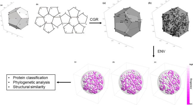
Graphical abstract

Highlights

• •This method is a novel numerical representation for proteins.
• •It includes 3-dimensional Chaos Game Representation and Extended Natural Vector.
• •The new method performs well on protein classification and phylogenetic analysis.
• •The method can reflect the differences of protein structure.

Abstract

Chaos Game Representation (CGR) was first proposed to be an image representation method of DNA and have been extended to the case of other biological macromolecules. Compared with the CGR images of DNA, where DNA sequences are converted into a series of points in the unit square, the existing CGR images of protein are not so elegant in geometry and the implications of the distribution of points in the CGR image are not so obvious. In this study, by naturally distributing the twenty amino acids on the vertices of a regular dodecahedron, we introduce a novel three-dimensional image representation of protein sequences with CGR method. We also associate each CGR image with a vector in high dimensional Euclidean space, called the extended natural vector (ENV), in order to analyze the information contained in the CGR images. Based on the results of protein classification and phylogenetic analysis, our method could serve as a precise method to discover biological relationships between proteins.

1. Introduction

The study of protein is always one of the core subjects in biology, because of the central role that proteins play in almost all biological processes. Considering the great variety of proteins and the huge expense of experimental study of molecular structure and function, it is unrealistic to analyze the biological function of every protein in the lab. Therefore, it is significant to obtain the similarity of proteins in structure and function from protein sequence analysis and predict functions based on the similarity [1]. As a foundation of protein sequence analysis, a proper numerical representation makes it more convenient to find and analyze the characteristics of those sequences. In recent years, many numerical representation methods have been proposed and then applied in protein classification, protein function prediction and search for target proteins with certain structures or biological functions [2], [3], [4].

With the huge increase of biological sequence data in recent years, numerical encoding methods are more demanding in computational efficiency. Among the methods proposed recently, natural vector method, which is proposed in [5], [6], is an efficient, alignment-free numerical encoding method of molecular sequences. With this method, every molecular sequence is associated with a vector in high dimensional space and the correspondence has been proved to be strictly one-to-one.

Apart from representing molecular sequences into numerical expression directly, many other numerical representations are constructed by first giving the sequence a graphical representation and then studying the image numerically [7]. Chaos game representation (CGR) was originally applied to bioinformatics as an image representation of DNA sequences by Jeffrey [8]. The four nucleotides (A, T, G, C) were put on the 4 vertices of the unit square, and every DNA sequence was mapped to a series of points inside the unit square in 2-dimensional space. While DNAs are composed of four kinds of nucleotides, proteins are made up of twenty kinds of amino acids. Thus, it remains to decide the distribution of the 20 amino acids when promoting CGR to the image representation of proteins.

Fisher et al. [9] first distributed the 20 amino acids on the vertices of a regular 20-sided polygon and then every protein was represented by a series of points inside the unit circle. Considering the limitation that a 20-vertex CGR cannot be used to demonstrate the similarity of homologous protein sequences with conservative substitutions, Basu et al. [10] proposed a 12-vertex CGR, with each vertex of a regular 12-sided polygon representing an amino acid with its conservative substitutions. The number of the vertices in CGR was then reduced to four [11], [12], with each vertex of a square representing one of the four groups of amino acids, that is, the non-polar, uncharged polar, negative polar and positive polar groups. The reduction in the vertices of CGR image can help represent the similarity in homologous protein sequences, however, these kinds of CGR is not a strictly one-to-one representation of protein sequence as in the case of DNA [8].

With the chaos game representation method, the study of molecular sequences is converted into the study of their CGR images. Since the frequency of points in a certain area in a CGR image represents the frequency of a certain string in the molecular sequence, Basu et al. [10] employed the grid-counting algorithm to compare different protein families. In order to study the frequency of points in a CGR image more intuitively, Almeida et al. [13] proposed the frequency matrices extracted from the CGR image of DNA, called the FCGR. The characteristic of a CGR image is then illustrated by a gray-scale image and has been studied by means of deep-learning in recent years [14]. Moreover, Pei et al. [16] associated each gray-scale image with a vector in high-dimensional Euclidean space, called the extended natural vector (ENV). The method combining FCGR and ENV performs well in entire genome comparison.

In this study, considering that the regular dodecahedron is one of the five known regular polyhedrons in three-dimensional Euclidean space and there are exactly 20 vertices on a regular dodecahedron. we choose to distribute the 20 amino acids on the vertices of a regular dodecahedron and obtain a novel three-dimensional CGR image for proteins, in which every protein sequence is mapped to a series of points in the regular dodecahedron in three-dimensional space. We have proved that each CGR image can only represent at most one protein sequence, which improved the limitation of previous CGR methods.

In the meanwhile, inspired by Pei et al.’s work [16], we construct a 160-dimensional vector, also called ENV, for each three-dimensional CGR image as well. With the help of ENV, the similarity of homologous protein sequences can also be illustrated by arranging the amino acids with similar properties next to each other on the vertices of the regular dodecahedron. In this way, homologous proteins will have similar CGR images in the sense that the ENVs of homologous proteins are closed to each other in the vector space.

Our method is first tested on several big families of proteins in the human proteome. The property that ENVs of proteins with similar amino acid sequences will cluster together in the vector space is confirmed by the fact that convex hulls of ENVs of different protein families do not intersect with each other. Then the Euclidean distance between ENVs is used to measure the biological distance between protein sequences. The distance between ENVs not only performs well on phylogenetic analysis, but is also positively correlated with the root mean square deviation (RMSD) of protein structures. The results show that our representation method is a more precise method to discover biological relationships between proteins than other methods on sequence comparison.

2. Methods

2.1. Three-dimensional Chaos Game Representation image

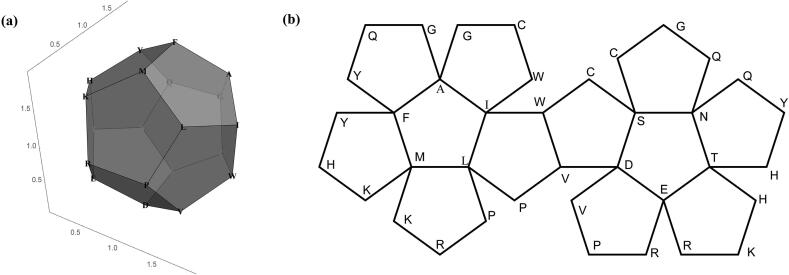
In mathematics, it was beautifully shown that there are only 5 regular polygons in $R^3$. They are the tetrahedron, cube, octahedron, dodecahedron, and icosahedron, the so-called the Platonic solids. The naturally given dodecahedron has exactly 20 vertices which coincide the number of amino acids for forming protein sequences. So it is natural to investigate the 3-dimensional representation of protein sequences by means of a dodecahedron. The first step to obtaining the three-dimensional CGR images of proteins is to decide the distribution of the 20 amino acids on the vertices of a dodecahedron. In this paper, we will use the abbreviation for the amino acids, that is, $\mathrm{\Omega }=(A,R,K,H,Y,T,S,G,Q,C,N,E,D,V,W,P,F,M,L,I)$, to represent both the amino acids and the corresponding vertices. We tried to put amino acids with similar properties together, so that ENVs of homologous proteins constructed later will cluster together in the vector space. The 20 amino acids can be naturally divided into 4 groups according to [12], (non-polar, positive polar, uncharged polar and negative polar). We put amino acids of non-polar ($A,I,L,M,F,P,W,V$). and uncharged polar group ($N,C,Q,G,S,T,Y$) on two adjacent faces respectively and amino acids from the other two groups, positive polar group ($R,H,K$) and negative polar group ($D,E$) are also distributed next to each other. Fig. 1 (a) shows the 3-dimensional images of the regular dodecahedron and the coordinates of each vertex are summarized in Table 1. Fig. 1 (b) shows the expanded image of a regular dodecahedron and the distribution of amino acids on the vertices is also marked on it.

Fig. 1.

Vertices with identical letters will coincide when folding into a regular dodecahedron. (a) Distribution of amino acids on the vertices of a regular dodecahedron (3-dimensional view). (b) Distribution of amino acids on the vertices of a regular dodecahedron (extended image).

Table 1.

Coordinates of the 20 amino acids on the vertices of a regular dodecahedron.

Amino acid	Coordinates
G	(1.3568,  1.9342,  1.0000)
Q	(0.6432,  1.9342,  1.0000)
P	(1.3568,  0.0658,  1.0000)
R	(0.6432,  0.0658,  1.0000)
I	(1.9342,  1.0000,  1.3568)
H	(0.0658,  1.0000,  1.3568)
W	(1.9342,  1.0000,  0.6432)
T	(0.0658,  1.0000,  0.6432)
F	(1.0000,  1.3568,  1.9342)
M	(1.0000,  0.6432,  1.9342)
S	(1.0000,  1.3568,  0.0658)
D	(1.0000,  0.6432,  0.0658)
A	(1.5774,  1.5774,  1.5774)
L	(1.5774,  0.4226,  1.5774)
C	(1.5774,  1.5774,  0.4226)
Y	(0.4226,  1.5774,  1.5774)
K	(0.4226,  0.4226,  1.5774)
N	(0.4226,  1.5774,  0.4226)
E	(0.4226,  0.4226,  0.4226)
V	(1.5774,  0.4226,  0.4226)

The three-dimensional CGR image of a protein is a series of points inside the regular dodecahedron inscribed to ball $\mathcal{B}$, which is centered at $(1,1,1)$ with radius $r=1$, where the points are iteratively generated by:

$$X_0=\left(1,1,1\right),X_n=\left(1-u\right)*{\omega }_n+u*X_{n-1},n⩾1$$ (1)

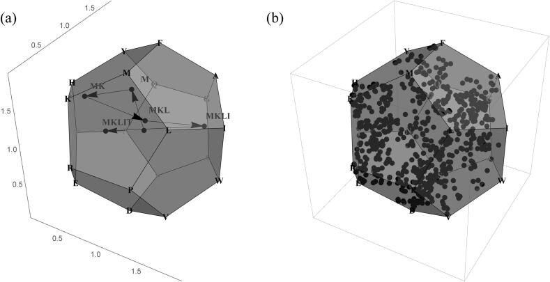
where u is a parameter to be determined, (although $u=\frac{1}{2}$ in the original two-dimensional CGR image for DNA), and ${\omega }_n\in \mathrm{\Omega },\left(n⩾1\right)$ is the nth amino acid in the protein sequence. Fig. 2 shows the process.

Fig. 2.

(a) Three dimensional Chaos Game Representation (CGR) of the first five amino acids of KNG1_HUMAN (P01042), “MKLIT”. (b) Three dimensional Chaos Game Representation (CGR) of KNG1_HUMAN (P01042).

Based on the iterative formula (1), the CGR image of a protein is determined by its amino acid sequence. In the meanwhile, with the parameter u chosen properly, the nth amino acid in a protein can also be deduced from the location of the nth point in a CGR image. In fact, if the parameter u is chosen so that with different nth amino acids, the areas that the nth point can be located in are separated from each other, then the nth point also determines the nth amino acid in a protein. This property of CGR image and its generalization are summarized and expressed mathematically in Theorem 1 below. For ease of theorem statement, we first introduce the following concept to denote the area that each point in CGR can be located in.

Definition 1

For each $\omega \in \mathrm{\Omega }$, one of the vertices of the regular dodecahedron, the ball centered at $X_{\omega }=u*(1,1,1)+(1-u)*\omega$ with radius u is called the ball controlled by amino acid $\omega$, and is denoted by ${\mathcal{B}}_{\omega }$.

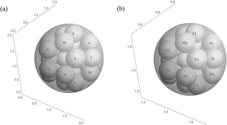
We can prove that the nth point in the CGR image $X_n$ will be located inside the ball controlled by ${\omega }_n$ and in the meanwhile, through rigorous mathematical calculation, with the parameter u chosen to be $u=\frac{\sqrt{5}-1}{\sqrt{5}+2\sqrt{3}-1}$, the balls controlled by different amino acids do not intersect with each other. More precisely, with u chosen above, the balls controlled by different amino acids are tangent to each other. (This property is also asserted in Theorem 1. (5) and the mathematical deduction is shown in supplementary files.) As a generalization of the above definition, we can also define the balls controlled by dipeptides which enjoy similar properties. The radius of ball is changed into $u^2$ in order to guarantee the non-intersection of balls controlled by different dipeptides.

Definition 2

For each dipeptide ${\omega }_1{\omega }_2,{\omega }_1,{\omega }_2\in \mathrm{\Omega }$, the ball centered at $X_{{\omega }_1{\omega }_2}=u*(1-u)*({\omega }_1-X_0)+X_{{\omega }_2}$with radius $u^2$ is called the ball controlled by dipeptide ${\omega }_1{\omega }_2$, and is denoted by ${\mathcal{B}}_{{\omega }_1{\omega }_2}$.

Fig. 3 shows an example of the above definition. The small balls in Fig. 3 (a) are the balls controlled by the 20 amino acids, and Fig. 3 (b) is an enlargement of ball ${\mathcal{B}}_L$. The small balls in Fig. 3 (b) are balls controlled by dipeptides ‘$\omega L$’.

Fig. 3.

(a) The ball controlled by 20 amino acids. (b) The ball ${\mathcal{B}}_L$ and the balls controlled by dipeptides ‘$\omega L$’.

With the two definitions above, we have the following theorem and the proof is shown in the supplementary files.

Theorem 1

For an amino acid sequence of length N, with $\{X_n:0⩽n⩽N\}$ and u defined above, CGR images have the following properties:

• (1) ${\mathcal{B}}_{\omega }$ is inscribed to the ball $\mathcal{B}$ at $\omega ,\forall \omega \in \mathrm{\Omega }$;

• (2) ${\mathcal{B}}_{{\omega }_1{\omega }_2}$ is inscribed to ${\mathcal{B}}_{{\omega }_2},\forall {\omega }_1,{\omega }_2\in \mathrm{\Omega }$;

• (3) $X_n\in {\mathcal{B}}_{{\omega }_n},\forall 1⩽n⩽N$;

• (4) $X_n\in {\mathcal{B}}_{{\omega }_{n-1}{\omega }_n},\forall 2⩽n⩽N$;

• (5) ${\mathcal{B}}_{{\omega }_1}\cap {\mathcal{B}}_{{\omega }_2}=\varnothing$, if ${\omega }_1\ne {\omega }_2$. More precisely, if ${\omega }_1$ and ${\omega }_2$ are adjacent vertices, then ${\mathcal{B}}_{{\omega }_1}$ and ${\mathcal{B}}_{{\omega }_2}$ are tangent to each other.

• (6) For a certain amino acid $\omega$, the number of $\omega$ in a protein is equal to the number of points in ${\mathcal{B}}_{\omega }$. Besides, for a certain dipeptide ${\omega }_1{\omega }_2$, the number of ${\omega }_1{\omega }_2$ in a protein is equal to the number of points in ${\mathcal{B}}_{{\omega }_1{\omega }_2}$.

• (7) For each $n\in \mathbb{N},1⩽n⩽N$, the first n amino acid in the protein is determined by $X_n$, that is, given the coordinates of $X_n$ in a CGR image, we can obtain the first n amino acids in the protein.

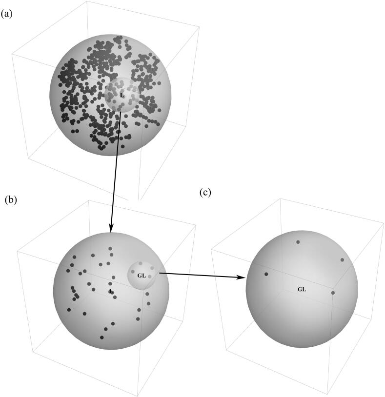
As an example, Fig. 4 shows the three-dimensional CGR image of Kininogen-1 (KNG1_HUMAN, entry number P01042 in Uniprot), a protein in human kidney with 644 amino acids. Fig. 4 (a) shows the location of points in the unit ball, (b) is an enlargement of ${\mathcal{B}}_L$, the ball controlled by amino acid L and (c) is an enlargement of ${\mathcal{B}}_{\mathit{GL}}$, the ball controlled by dipeptide GL. In Fig. 4 (c), there are four points contained in ${\mathcal{B}}_{\mathit{GL}}$ , which means that the dipeptide GL exists four times in the protein KNG1_HUMAN.

Fig. 4.

Three-dimensional CGR image of KNG1_HUMAN. (a) shows the location of points in the ball $\mathcal{B}$, (b) is an enlargement of ${\mathcal{B}}_L$, and (c) is an enlargement of ${\mathcal{B}}_{\mathit{GL}}$.

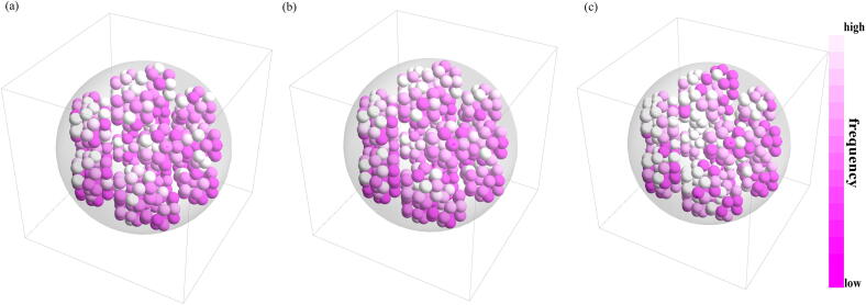
With the help of three-dimensional CGR images, we can intuitively count the number of occurrence of a certain amino acid or dipeptide in a protein and compare the frequency of different amino acids or dipeptides qualitatively. Fig. 5 shows the three-dimensional CGR image of three different KNG1_HUMAN (P01042), KNG2_BOVIN (P01045) and UROM_HUMAN (P07911). From Fig. 5, we can see that the three-dimensional CGR images of KNG1_HUMAN (P01042) and KNG2_BOVIN (P01045), which are both a kind of kininogen serving to be an inhibitor of thiol proteases, are more similar; while the three-dimensional CGR image of UROM_HUMAN (P07911) is different from others, and the biological function of this protein is promoting the formation of complex filamentous gel-like structure of the apical membrane of certain cells, which is also different from the other two proteins.

Fig. 5.

Three-dimensional CGR image of (a) KNG1_HUMAN (P01042), (b) KNG2_BOVIN (P01045) and (c) UROM_HUMAN (P07911).

Nevertheless, in order to analyze the CGR image quantitatively and mine more information about proteins from their CGR images, we need to associate each CGR image with an ENV that can summarize the information contained in the CGR image.

2.2. Construction of the Extended Natural Vector

The ENV we constructed in this study is a vector obtained by integrating information of dipeptides contained in a CGR image. It can help summarize the properties of a CGR image and reflect the characteristics of the amino acid sequence represented by the image. The ENV corresponding to a CGR image can be built with the following steps.

• 1.For a given three-dimensional CGR image, we count the frequency of points in each of the ball controlled by the 400 dipeptides, and thus, according to Theorem 1. (6), we get the frequency of each dipeptide in the amino acid sequence.
• 2.Divide the 400 kinds of dipeptides into at most 16 groups according to the frequency. Dipeptide occurring least is assigned to group 1, while the most frequent dipeptide is assigned to group 16. The group of other dipeptides is linearly correlated to their frequency.
  More precisely, the frequency of dipeptide ${\omega }_1{\omega }_2$ is recorded as $a_{{\omega }_1{\omega }_2},{\omega }_1,{\omega }_2\in \mathrm{\Omega }$. Denote $M=\max \{a_{{\omega }_1{\omega }_2}:{\omega }_1,{\omega }_2\in \mathrm{\Omega }\}$ and $m=\min \{a_{{\omega }_1{\omega }_2}:{\omega }_1,{\omega }_2\in \mathrm{\Omega }\}$. Then the group number k ($1⩽k⩽16$) of ${\omega }_1{\omega }_2$ is determined by the following formula:

  $$k=\mathit{round}\left(\frac{15}{M-m}\right(a_{{\omega }_1{\omega }_2}-m)+1)$$ (2)

  where $\mathit{round}\left(x\right)$ means the integer nearest to x.

  In our example of protein KNG1_HUMAN, dipeptide ‘HW‘ exists most often (15 times) and thus, is assigned to group 16, while 127 dipeptides do not exist in the protein. Therefore, for KNG1_HUMAN, $M=15$ and $m=0$. Because dipeptide ’GL’ exists 4 times, it is assigned to group 5. The number of dipeptides in each group is summarized in Table 2.

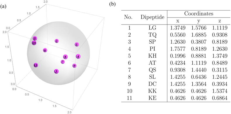
  Eleven dipeptides (‘LG‘, ‘TQ’, ‘SP’, ‘PI’, ‘KH’, ‘AT’, ‘QS’, ‘SL’, ‘DC’, ‘KK’, ‘KE’) are assigned to group 7 and Fig. 6 shows the 11 balls controlled by dipeptides in group 7 of KNG1_HUMAN (P01042). The coordinates of the center of the each ball are also summarized in Fig. 6.

• 3.The first group of components in the ENV are $f_1,f_2,\dots ,f_{16}$, where $f_i=\frac{n_i}{400},1⩽i⩽16$ and $n_i$ is the number of dipeptides in group i. Some of $n_i,(i=1,2,\dots ,16)$, could be 0. In our example, we have $n_1=0.3175,n_2=0.2650,\dots ,n_7=0.0275,\dots ,n_{16}=0.0025$.
• 4.
  The second group of components in the ENV are mean locations ${\mu }_{1,i},{\mu }_{2,i},\dots ,{\mu }_{3,i},i=1,2,\dots ,16$ of each group.

  $$\begin{array}{c}{\mu }_{1,i}=\frac{1}{n_i}\sum _{s\in \mathrm{Group}i}{x}_{s,i},{\mu }_{2,i}=\frac{1}{n_i}\sum _{s\in \mathrm{Group}i}{y}_{s,i},{\mu }_{3,i}=\frac{1}{n_i}\sum _{s\in \mathrm{Group}i}{z}_{s,i}\end{array}$$ (3)

  where $(x_{s,i},y_{s,i},z_{s,i})$ is the coordinates of the center of the ball controlled by dipeptide s. Define $({\mu }_{1,i},{\mu }_{2,i},{\mu }_{3,i})=(0,0,0)$ if $n_i=0$. In the example of protein KNG1_HUMAN, according to Fig. 6, we have

  $$({\mu }_{1,7},{\mu }_{2,7},{\mu }_{3,7})=(0.9347,0.9849,0.9565)$$ (4)
• 5.
  The third group of components in the ENV are the normalized second order central moments.

  $$D_{i,r,s,u}=\sum _{t\in \mathrm{Group}i}\frac{{\left(x_{t,i}-{\mu }_{1,i}\right)}^r{\left(y_{t,i}-{\mu }_{2,i}\right)}^s{\left(z_{t,i}-{\mu }_{3,i}\right)}^u}{n_i}$$ (5)

  where $i=0,1,2,\dots ,15,\left(r,s,u\right)$ = (2, 0, 0), (0, 2, 0), (0, 0, 2), (1, 1, 0), (1, 0, 1), (0, 1, 1).
  In the example of protein KNG1_HUMAN, according to Fig. 6. again, we have

  $$\begin{array}{cc}\hfill & (D_{7,2,0,0},D_{7,0,2,0},D_{7,0,0,2},D_{7,1,1,0},D_{7,1,0,1},D_{7,0,1,1})=\hfill \\ \hfill & (0.2592,0.2067,0.1410,0.0156,-0.0224,-0.0649)\hfill \end{array}$$ (6)
  Now, we get the 160-dimensional ENV of a three-dimensional CGR image,

  $$\begin{gathered} (f_1,f_2,\dots ,f_{16};{\mu }_{1,1},{\mu }_{1,2},\dots ,{\mu }_{1,16}; \\ {\mu }_{2,1},{\mu }_{2,2},\dots ,{\mu }_{2,16};{\mu }_{3,1},{\mu }_{3,2},\dots ,{\mu }_{3,16}; \\ {D}_{1,2,0,0},D_{2,2,0,0},\dots ,D_{16,2,0,0};D_{1,0,2,0},D_{2,0,2,0},\dots ,D_{16,0,2,0}; \\ {D}_{1,0,0,2},D_{2,0,0,2},\dots ,D_{16,0,0,2};D_{1,1,1,0},D_{2,1,1,0},\dots ,D_{16,1,1,0}; \\ {D}_{1,1,0,1},D_{2,1,0,1},\dots ,D_{16,1,0,1};D_{1,0,1,1},D_{2,0,1,1},\dots ,D_{16,0,1,1}) \end{gathered}$$ (7)

Table 2.

The number of dipeptides in each group of KNG1_HUMAN (P01042).

Group	1	2	3	4	5	6	7	8
Number of dipeptides	127	106	75	38	27	13	11	0
Group	9	10	11	12	13	14	15	16
Number of dipeptides	1	0	0	1	0	0	0	1

Fig. 6.

Balls controlled by dipeptides in group 7 of KNG1_HUMAN (P01042).

2.3. Distance measure

For two different amino acid sequences,we can construct their 160- dimensional ENV $V_1=(p_1,p_2,\dots ,p_{160})$ and $V_2=(q_1,q_2,\dots ,q_{160})$, where $p_i$ and $q_i$ are defined in (7). The biological distance of the two amino acid sequences is represented by the 160-dimensional Euclidean distance of their ENVs.

2.4. Convex hull analysis

The distance from a vector to a convex hull can be calculated by a quadratic optimization solution:

$$D^2=\min |Y-{\displaystyle \sum _{i=1}^n}{\lambda }_i{X}_i{|}^2,0⩽{\lambda }_i⩽1,{\displaystyle \sum _{i=1}^n}{\lambda }_i=1$$ (8)

where Y denotes a vector in the space, $X_i,i=1,2,\dots ,n$ are members in a vector set, and n is the size of the vector set.

The distance of two convex hulls can also be calculated by a quadratic optimization solution:

$$\begin{gathered} D^2=min|\sum _{i=1}^m{\lambda }_i{X}_i-\sum _{j=1}^n{\mu }_j{Y}_j{|}^2,0⩽{\lambda }_i,{\mu }_j⩽1, \\ s.t.\sum _{i=1}^m\lambda =\sum _{j=1}^n{\mu }_j=1 \end{gathered}$$ (9)

where $X_i,i=1,2,\dots ,m,Y_j,j=1,2,\dots ,n$, are members in two vector sets, and $n,m$ are the size of the vector sets.

2.5. Other methods

When applying our methods into phylogeny analysis, we use the principle of UPGMA to construct the phylogenetic tree. We also make a comparison between our methods and the Natural Vector method.

2.5.1. Natural vector (NV) method

Let $S=s_1{s}_2\dots s_n$ be an amino acid sequence of length n and $s_i\in \mathrm{\Omega },i=1,2,\dots ,n$. For $K\in \mathrm{\Omega }$, we define $w_K:\mathrm{\Omega }\to \{0,1\}$,

$$w_K\left(s_i\right)=\left\{\begin{array}{cc}1\hfill & s_i=K\hfill \\ 0\hfill & s_i\ne K\hfill \end{array}\right)$$ (10)

• 1.The first group of components in NV contains the number of amino acid K in the amino acid sequence $S:n_K={\sum }_{i=1}^n{w}_K\left(s_i\right)$.
• 2.The second group of components in NV contains the mean position of amino acid $K:{\mu }_K={\sum }_{i=1}^n\frac{i*w_K\left(s_i\right)}{n_K}$.
• 3.The third group of components in NV contains the scaled variance of positions of amino acid $K:D_2^K={\sum }_{i=1}^n\frac{{(i-{\mu }_K)}^2{w}_K\left(s_i\right)}{n*n_K}$

The 60-dimensional NV of an amino acid sequence S is defined by $(n_A,n_R,\cdots ,n_I,{\mu }_A,{\mu }_R,\cdots ,{\mu }_I,D_2^A,D_2^R,\cdots ,D_2^I)$.

3. Results

3.1. Application in protein classification

According to Fig. 5, proteins with similar biological functions and similar amino acid sequences have similar CGR images. Based on the construction of ENV, the distance between these proteins are also relatively short. Since homologous proteins (proteins in the same protein family, superfamily or class) enjoy similar amino acid sequences, we can classify proteins without family information by the following steps:

• Step 1. For a protein without family information, we can first find all the families that the protein can possibly belong to. In order to improve the accuracy of the classification, the alternative families are supposed to be as few as possible.

• Step 2. Collect all the proteins in the alternative families and construct the CGR image and the corresponding ENV of each protein.

• Step 3. Calculate the distance between the ENV of the protein to be classified and the convex hull of each alternative family by solving the quadratic optimization problem (8). The protein without family information can be regarded as a member of the family with the shortest distance.

3.1.1. Classification results of human protein groups

Human proteome dataset in UniprotKB contains 74,034 proteins. Among them, 20,350 proteins in SwissProt have been manually annotated. Except for proteins without family information, 14,303 proteins are divided into 5048 classes, superfamilies, families and subfamilies. While 2832 groups contain only one protein and 925 groups contain only two proteins, big groups are composed of more than 50 proteins and there are 671 proteins in the biggest group, G-protein coupled receptor 1 family.

To evaluate the accuracy of this protein classification method, we applied it on some groups of proteins from human proteome. Each group contains proteins from a certain protein family, superfamily or class, and thus proteins in each group have similar amino acid sequences. The number of proteins in each group is summarized in Table 3.

Table 3.

Ten groups of proteins analyzed in this study and the number of proteins in each group.

No.	Protein group	Number of proteins
1	G-protein coupled receptor 1 family	671
2	Protein-tyrosine phosphatase family	93
3	Krueppel C2H2-type zinc-finger protein family	537
4	TRAFAC class	175
5	Small GTPase superfamily	162
6	Immunoglobulin superfamily	130
7	Protein kinase superfamily	490
8	Peptidase S1 family	119
9	Major facilitator (TC 2.A.1) superfamily	99
10	Glycosyltransferase 10 family	159

For two different protein groups, we keep about 10% retained proteins in each group as proteins without family information and use the rest to construct the convex hull of each protein family. We first calculate the distance between convex hulls of the two protein groups by solving the quadratic optimization in (9). The results in Table 4 shows that each two convex hulls have strictly positive distance and thus do not intersect with each other. The retained proteins are assigned to one of the protein families according to the above protein classification method. To evaluate the performance of this classification method, we calculate the accuracy and AUC (area under the curve) of each classification. In order to compare our 3D-CGR with the existing 2D-CGR images, we apply SVM (support vector machine) to the existing 2D-CGR images proposed by Lochel et al. [14] and use this method to classify the proteins again. The results are summarized in Tables 4 and 5. The confusion matrices of these classifications are shown in supplementary files.

Table 4.

The classification accuracy of 5 selected pairs of protein groups.

Protein group	Number of Proteins	Number of Retained Proteins	AUC	Convex hull Distance
Classification 1
G-protein coupled receptor 1 family	671	67	0.7960	0.0481
Protein-tyrosine phosphatase family	93	9
Classification 2
Krueppel C2H2-type zinc-finger protein family	537	54	0.9198	0.0249
TRAFAC class	175	18
Classification 3
Small GTPase superfamily	162	16	0.9231	0.0211
Immunoglobulin superfamily	130	13
Classification 4
Protein kinase superfamily	490	49	0.8622	0.0112
Peptidase S1 family	119	12
Classification 5
Major facilitator (TC 2.A.1) superfamily	99	9	0.8741	0.0835
Glycosyltransferase 10 family	159	15

Table 5.

Accuracy of classifications using 2D-CGR & SVM and 3D-CGR & ENV (our method).

Classification No.	Accuracy
	2D-CGR & SVM	3D-CGR & ENV (our method)
Classification 1	100%	96.05%
Classification 2	94.44%	95.83%
Classification 3	93.10%	100%
Classification 4	96.72%	91.80%
Classification 5	88.46%	91.67%
Mean accuracy	94.54%	95.07%

As another comparison, instead of considering the convex hull, we also try k-nearest neighborhood (KNN) method in protein classification. The performance of KNN method is not better than the method considering the convex hull and the detailed classification results are also shown in supplementary files.

Tables 4 and 5 show that the mean accuracy of the five classifications using our method is higher than the result using 2D-CGR method. Besides, if the number of alternative families that a protein can possibly belongs to can be sufficiently narrowed down in advance, we can use our method to complete the classification with high accuracy. In practice, further classification information of proteins in a certain family can also be obtained with our method.

3.1.2. Classification of protein kinase C family

In order to further apply and test our protein classification method, we classified protein kinase C (PKC) family by our method. PKC is a family of enzymes, which can regulate protein activities and cellular responses [15]. The PKC family can be biologically divided into 3 groups, that is atypical protein kinase C (aPKC), novel protein kinase C (nPKC) and conventional protein kinase C (cPKC). In our dataset, there are 257 aPKCs, 297 cPKCs and 190 nPKCs. We also retained about 10% PKCs in each group as PKCs with unknown classification and use the rest to construct the convex hull of aPKC, cPKC and nPKC subfamilies. The classification result is shown in Table 6.

Table 6.

The classification accuracy result of Protein Kinase C family.

PKC group	Number of PKCs	Number of retained PKCs	Classification accuracy	Average accuracy
aPKC	257	26	100%	98.67%
cPKC	297	30	100%
nPKC	190	19	94.74%

3.2. Phylogeny analysis

Influenza A viruses are negative-sense, single-stranded, segmented RNA viruses. They are a constant threat to the health of human and animal because of their high mutation rate [17]. In this study, according to the taxonomy information in Uniprot, we collect all the manually reviewed proteins of 22 Influenza A viruses from 5 subtypes in Swiss-prot database. In order to use the information from the entire proteome of viruses from each subtype, we connect all the proteins from one kind of virus into a single amino acid sequence, called the connected amino acid sequence. Because the ENV is determined by the frequency of each dipeptide, the order of the connection makes little difference in the ENV of each subtype. In the meanwhile, we can obtain the NV of the connected amino acid sequence.

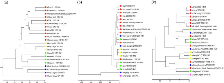
We calculate the distance matrices of ENV method and NV method and use the principle of UPGMA to construct the phylogenetic tree of the 22 Influenza A viruses. In the meanwhile, we also apply the Clustal W method on the connected amino acid sequences, in order to make a comparison with traditional alignment-based methods. As is shown in Fig. 7, the phylogenetic tree constructed by our ENV method can demonstrate the phylogeny process more accurately, since it can properly classify each subtype.

Fig. 7.

Phylogenetic tree constructed by our method, NV method and traditional alignment method. (a) is the tree of our method, (b) is the tree of NV method and (c) is the tree of Clustal W method.

The result of phylogeny analysis shows that as an alignment-free method, our method can deal with the information of several sequences simultaneously. Therefore, our method may have application prospect in comparison among protein families or proteome.

3.3. Relationship between structural similarity and ENV distance

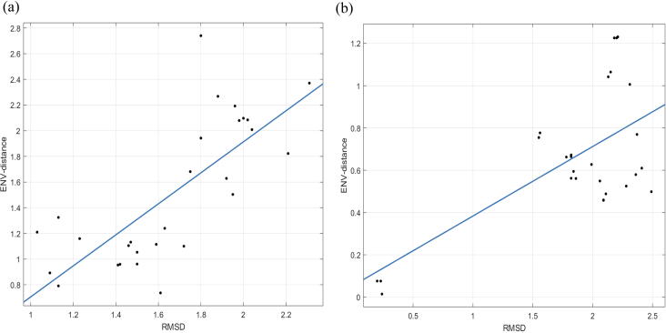
According to the research above, the distance between ENVs can reflect the similarity of protein sequences. The less similar the two protein sequences are, the greater the pairwise distance between the corresponding ENVs is. And the root mean square deviation (RMSD) of protein structure is often used to measure the protein structural similarity, and higher values represent more different structures [18]. Based on the principle that the protein structure is closely related to its sequence, the RMSD and the ENV-distance should be positively correlated.

First, we calculate the ENV-distance matrix X of protein sequences and the RMSD matrix Y of protein structures. The pairwise similarity matrix by Clustal W is calculated for comparison [19]. The Pearson correlation cor of two distance matrices is calculated to measure the relationship as follows.

$$\mathit{cor}=\frac{{\displaystyle \sum _{i=1}^n}(X_i-\bar{X})(Y_i-\bar{Y})}{\sqrt{{\displaystyle \sum _{i=1}^n}{(X_i-\bar{X})}^2}\sqrt{{\displaystyle \sum _{i=1}^n}{(Y_i-\bar{Y})}^2}}$$ (11)

where n is the number of elements of the upper triangular of the distance matrices, $\bar{X}$ and $\bar{Y}$ are means of X and Y, respectively.

Two datasets with different sequence lengths are used to analyze the relationship. The first dataset includes 8 serine hydroxymethyltransferase proteins with the lengths of about 420 amino acids, and the second dataset includes 8 response regulator proteins with the lengths of about 100 amino acids. For the first dataset, the Pearson correlation between the matrices of the ENV-distance and the RMSD is 0.752, while that between the matrices of the sequence similarity by Clustal W and the RMSD is 0.183. For the second dataset, the Pearson correlation between the matrices of the ENV-distance and the RMSD is 0.648, while that between the matrices of the sequence similarity by Clustal W and the RMSD is 0.146. The Pearson correlation between the matrices of the ENV-distance and the RMSD is larger than the matrices of the sequence similarity by Clustal W and the RMSD for both datasets. So the RMSD and the ENV-distance are correlated more significantly than the RMSD and the sequence similarity by Clustal W.

We take the RMSD as the x-axis and the ENV-distance as the y-axis to perform linear regression. As shown in Fig. 8, the linear correlation between the ENV-distance and RMSD clearly provides evidence of the positive correlation between RMSD and ENV distance.

Fig. 8.

Linear regression of RMSD of a pair of protein structures and ENV distance of the corresponding protein sequences; the RMSD as the x-axis and the ENV-distance as the y-axis (a) dataset 1: 8 serine hydroxymethyltransferase proteins (b) dataset 2: 8 response regulator proteins.

4. Discussion

In this study, we propose a novel numerical representation method for proteins. Firstly, amino acid sequences are transformed into a CGR image in three-dimensional space. Since proteins are made up of twenty kinds of amino acids and coincidentally, a regular dodecahedron consists of twenty vertices, we decide to distribute each amino acid on a vertex of regular dodecahedron and transform the protein into a sequence of points inside the regular dodecahedron. We have proved that the sequence of points is uniquely determined by the protein, and thus, the study of amino acid sequence can be converted to the study of its three-dimensional CGR image.

Next, in order to quantitatively analyze the information contained in the CGR images, we construct the ENV for each image. With the help of CGR images and ENV, the information of protein sequences is converted to a 160-dimensional vector in Euclidean space, and thus, the features of proteins can be studied with mathematical instruments.

We try our method on several datasets and the results show that the ENVs of homologous proteins tend to cluster together in the 160-dimensional Euclidean space. This property can be applied to the classification of proteins without family information. We design a method of protein classification based on the above property and obtain classification results with high accuracy.

Besides, our method can also be used in phylogeny analysis. Rather than analyzing the distance among a certain protein from different species, our method can analyze a group of proteins simultaneously by connecting the proteins into a long sequence. The construction of ENV guarantees that the ENV won’t change much if we change the order of the connection.

We also analyze the relationship of RMSD of protein structures and ENV-distance of protein sequences. It indicates that to a certain extent the RMSD of protein structures is positively correlated with ENV-distance of protein sequences.

We compare the results of protein classification and phylogeny analysis with those of NV method. In the case of a single amino acid sequence, the NV method performs equally well with our method. However, when it comes to the case of a group of proteins, the NV method did not gather complete information from the sequences, because it only measures the single amino acid’s number and position but ignores the information of dipeptides.

For the data we analyze in this study, the length of most single amino acid sequence is less than 1000 and the connected sequence we analyze for phylogeny analysis is about 4000. Since 20 amino acids can form at most 400 dipeptides, it is suitable in our study to consider the frequency of dipeptides in a sequence. Nevertheless, when analyzing longer connected amino acid sequences, our method can also be applied. The only change we need to do is to consider the frequency of other short peptide, say tripeptide or tetrapeptide when constructing the ENV of the CGR images.

5. Data access

We constructed the CGR images and ENVs of proteins from three datasets in Uniprot. The ENVs are then used in protein family classification as well as phylogeny reconstruction.

Dataset 1 is composed of 5 families (G-protein coupled receptor 1, Krueppel C2H2-type zinc-finger, Protein-tyrosine phosphatase, Glycosyltransferase 10 and Peptidase S1), 4 superfamilies (Small GTPase, Protein kinase, Major facilitator (TC 2.A.1) and Immunoglobulin) and 1 class (TRAFAC) of proteins from human proteome. There are 2635 proteins in total and the number in each group is at least 93.

Dataset 2 contains proteins from a protein family, Protein Kinase C (PKC), which can be divided into three subfamilies, that is atypical protein kinase C (aPKC), nPKC and cPKC. In our dataset, there are 257 aPKCs, 297 cPKCs and 190 nPKCs.

Dataset 3 contains proteins of 22 Influenza A viruses. They are composed of 5 subtypes (11 H1N1, 4 H2N2, 3 H3N2, 3 H5N1 and 1 H7N3), according to the taxonomy in Uniprot.

Dataset 4 contains 8 serine hydroxymethyltransferase proteins and 8 response regulator proteins. The structures and sequences of these proteins are from RCSB dataset (https://www.rcsb.org/).

All the accession numbers of the dataset mentioned above are in supplementary files.

Declaration of Competing Interest

The authors declare that they have no known competing financial interests or personal relationships that could have appeared to influence the work reported in this paper.

CRediT authorship contribution statement

Zeju Sun: Methodology, Software, Data curation, Writing - original draft. Shaojun Pei: Methodology, Software, Visualization, Writing - review & editing. Rong Lucy He: Project administration, Validation. Stephen S.-T. Yau: Conceptualization, Supervision, Project administration, Funding acquisition.

Supplementary data

The following are the Supplementary data to this article:

References

- 1.Rigden D.J. Springer; Netherlands: 2017. From protein structure to function with bioinformatics. [Google Scholar]
- 2.Jurtz V.I., Johansen A.R., Nielsen M., Armenteros J.J.A., Nielsen H., Sonderby C.K., Winther O., Sonderby S.K. An introduction to deep learning on biological sequence data: examples and solutions. Bioinformatics. 2017;33:3685–3690. doi: 10.1093/bioinformatics/btx531. [DOI] [PMC free article] [PubMed] [Google Scholar]
- 3.Li J., Koehl P. 3D representations of amino acids applications to protein sequence comparison and classification. Comput Struct Biotechnol J. 2014;11:47–58. doi: 10.1016/j.csbj.2014.09.001. [DOI] [PMC free article] [PubMed] [Google Scholar]
- 4.Li B., Cai L., Liao B., Fu X., Bing P., Yang J. Prediction of protein subcellular localization based on fusion of multi-view features. Molecules. 2019;24:919. doi: 10.3390/molecules24050919. [DOI] [PMC free article] [PubMed] [Google Scholar]
- 5.Deng M., Yu C., Liang Q., He R.L., Yau S.S.T. A novel method of characterizing genetic sequences: genome space with biological distance and applications. PloS One. 2011;6 doi: 10.1371/journal.pone.0017293. [DOI] [PMC free article] [PubMed] [Google Scholar]
- 6.Yu C., Deng M., Cheng S.Y., Yau S.C., He R.L., Yau S.S.T. Protein space: a natural method for realizing the nature of protein universe. J Theor Biol. 2013;318:197–204. doi: 10.1016/j.jtbi.2012.11.005. [DOI] [PubMed] [Google Scholar]
- 7.Almeida J.S. Sequence analysis by iterated maps, a review. Brief Bioinf. 2014;15:369–375. doi: 10.1093/bib/bbt072. [DOI] [PMC free article] [PubMed] [Google Scholar]
- 8.Jeffrey H.J. Chaos game representation of gene structure. Nucl Acids Res. 1990;18:2163–2170. doi: 10.1093/nar/18.8.2163. [DOI] [PMC free article] [PubMed] [Google Scholar]
- 9.Fiser A., Tusnady G.E., Simon I. Chaos game representation of protein structures. J Mol Graph. 1994;12:302–304. doi: 10.1016/0263-7855(94)80109-6. [DOI] [PubMed] [Google Scholar]
- 10.Basu S., Pan A., Dutta C., Das J. Chaos game representation of proteins. J Mol Graph Model. 1997;15:279–289. doi: 10.1016/s1093-3263(97)00106-x. [DOI] [PubMed] [Google Scholar]
- 11.Yu Z., Anh V., Lau K. Chaos game representation of protein sequences based on the detailed HP model and their multifractal and correlation analyses. J Theor Biol. 2004;226:341–348. doi: 10.1016/j.jtbi.2003.09.009. [DOI] [PubMed] [Google Scholar]
- 12.Gao J. Early-warning model of influenza a virus pandemic based on principal component analysis. Appl Ecol Environ Res. 2017;15:891–899. [Google Scholar]
- 13.Almeida J.S., Carrico J.A., Maretzek A., Noble P.A., Fletcher M. Analysis of genomic sequences by Chaos Game Representation. Bioinformatics. 2001;17:429–437. doi: 10.1093/bioinformatics/17.5.429. [DOI] [PubMed] [Google Scholar]
- 14.Loechel H.F., Eger D., Sperlea T., Heider D. Deep learning on Chaos Game Representation for proteins. Bioinformatics. 2020;36:272–279. doi: 10.1093/bioinformatics/btz493. [DOI] [PubMed] [Google Scholar]
- 15.Wang Y., Tian K., Yau S.S.T. Protein sequence classification using natural vector and convex Hull method. J Comput Biol. 2019;26:315–321. doi: 10.1089/cmb.2018.0216. [DOI] [PubMed] [Google Scholar]
- 16.Pei S., Dong W., Chen X., He R.L., Yau S.S.T. Fast and accurate genome comparison using genome images: the extended natural vector method. Mol Phylogen Evol. 2019;141 doi: 10.1016/j.ympev.2019.106633. 106633. [DOI] [PubMed] [Google Scholar]
- 17.Pei S., Dong R., He R.L., Yau S.S.T. Large-scale genome comparison based on cumulative fourier power and phase spectra: central moment and covariance vector. Comput Struct Biotechnol J. 2019;17:982–994. doi: 10.1016/j.csbj.2019.07.003. [DOI] [PMC free article] [PubMed] [Google Scholar]
- 18.Taylor W.R., Orengo C.A. Protein structure alignment. J Mol Biol. 1989;208(1):1–22. doi: 10.1016/0022-2836(89)90084-3. [DOI] [PubMed] [Google Scholar]
- 19.Larkin MA., Blackshields G, Brown NP, Chenna R, Mcgettigan PA, Mcwilliam H, et al. Clustal W and clustal X version 2.0. Bioinformatics 23(21): 2007; 2947–2948. [DOI] [PubMed]
Associated Data
This section collects any data citations, data availability statements, or supplementary materials included in this article.