Probabilistic approximation of effective reproduction number of COVID-19 using daily death statistics

Abstract

The effective reproduction number (R) which signifies the number of secondary cases infected by one infectious individual, is an important measure of the spread of an infectious disease. Due to the dynamics of COVID-19 where many infected people are not showing symptoms or showing mild symptoms, and where different countries are employing different testing strategies, it is quite difficult to calculate the R, while the pandemic is still widespread. This paper presents a probabilistic methodology to evaluate the effective reproduction number by considering only the daily death statistics of a given country. The methodology utilizes a linearly constrained Quadratic Programming scheme to estimate the daily new infection cases from the daily death statistics, based on the probability distribution of delays associated with symptom onset and to reporting a death. The proposed methodology is validated in-silico by simulating an infectious disease through a Susceptible-Infectious-Recovered (SIR) model. The results suggest that with a reasonable estimate of distribution of delay to death from the onset of symptoms, the model can provide accurate estimates of R. The proposed method is then used to estimate the R values for two countries.

1. Introduction

The basic reproduction number R₀, which is the mean number of secondary cases generated by a typical infectious individual in a fully susceptible environment [1], is an established measure within the circles of epidemiology. The effective reproduction number (R), on the other hand, is the average number of secondary cases per infectious case in a population made up of both susceptible and non-susceptible (immune) hosts [2]. Meta-analysis of existing estimates of basic reproduction number for COVID-19 ranges from 1.9 to 6.5, with most studies agreeing of a value between 2 and 3 [3]. The knowledge of R₀ or R, provides the basis for further inference of different dynamics such as the effects of suppression policies adapted by different governments. This measure is often associated with compartmental models that simulate the outbreaks and spread of diseases. These models are commonly referred to as Susceptible-Infectious-Recovery (SIR) or Susceptible-Exposed-Infectious-Recovery (SEIR) models. Such models have been extensively used to model the current pandemic on COVID-19 [4,5].

Using COVID-19 data on cases in Wuhan and international cases that originated from Wuhan, Kucharski et al. [4] estimated median daily reproduction number (R) using astochastic transmission dynamic model (using SEIR compartments). Delays from symptom onset to reporting and uncertainty in case observation were accounted for in the model. Disease transmission was modelled as a geometric random walk process and sequential Monte Carlo simulation estimated the transmission rate over time, number of cases and the time-varying R. Zhang et al. [6] estimated R₀ in the early stage of COVID-19 outbreak on the Diamond Princess cruise ship. The R0 distribution was attained from the Maximum Likelihood estimation using a function in R and a bootstrap strategy was used to get a set of plausible R₀ values. A case-specific model for COVID-19 called θ-SEIHRD was proposed by Ivorra et al. [7], which is a deterministic model expanding on an existing SEIR model by including the additional new components: infectious but undetected; hospitalized or in quarantine at home that will recover; hospitalized that will die; and dead by COVID-19. The model also divides the recovered component into two: recovered after previously being detected as infectious and recovered after previously being infectious but undetected.

There are few studies that use other mathematical approaches than SIR or SEIR to estimate R or R₀. Diekmann et al. [8] defined R₀ as the dominant eigenvalue of Next Generation Matrices (NGM) for compartmental systems. The paper concluded that R₀>1 if and only if the real time exponential growth rate in the early stage of outbreak (r) > 0 and R₀=1 if r = 0. A graph theoretic form of gaussian elimination model was proposed in [9] to calculate the basic reproduction number. Using mortality data to calculate R values is also an interesting approach, which was demonstrated in application to the 1918 influenza pandemic in [10].

The objective of this study is to approximate the effective reproduction number (R) of an infectious disease, such as COVID-19 in a population, given the daily statistics released by authorities, as well as considering various studies that have been published on the early dynamics of COVID-19. This paper proposes a data-driven probabilistic method to approximate the R value of COVID-19, by utilizing the daily death statistics, and utilizing statistical studies on early dynamics of Covid-19.

2. The methodology

The objective of the proposed methodology is to approximate the effective reproduction number of any mortal infectious disease such as COVID-19, during the course of the pandemic, by utilizing the daily death statistics. The proposed model predicated on the basis that when the healthcare capacity is not reached in a country, the death rate (or the case-fatality ratio) from Covid-19 is a constant.

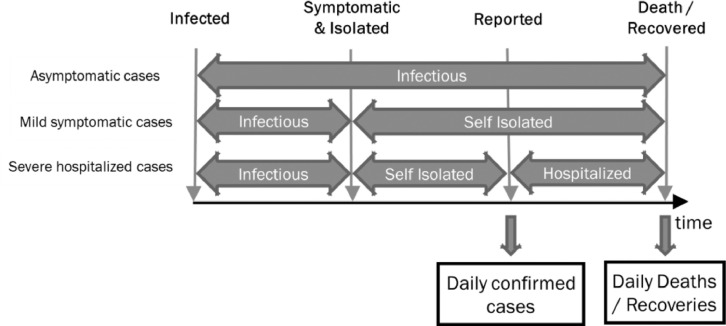
The proposed model considers the patient journey, and different patient types who are infected by the COVID-19 virus as depicted in the Fig. 1 . A person can be infected with the virus but show no symptoms at all. There is a delay between some person becoming infectious till the onset of symptoms. At this point, the person is expected to be isolated and not infect any more people. Furthermore, there is a delay between an isolated person that has been reported, and the death of a person. The process that a person goes through from infection to recovery from Covid-19 is illustrated in Fig. 1.

Fig. 1.

Different categories of COVID-19 patients. Depending on the testing strategy of a country, only certain categories of patients may be tested.

There are two main components of the proposed methodology to calculate the effective reproduction number. Firstly, the estimation of number of cases infected in a given day, to include those who are reported/confirmed with COVID-19, those who have symptoms and isolate, and those who do not have symptoms. Secondly, the calculation of effective reproduction number for each day from the number of people infected per day. The following subsections explain these components in detail.

The proposed measure to approximate effective reproduction number, denoted as R, is explained in the following sections. The effective reproduction number is defined as the average number of secondary cases infected by one person. In the following sections we derive the formulae for calculating the R for any given day.

The derivations in the proceeding subsections are based on the following definition of terms.

• • N(t): number of newly infected cases on day t
• • D(t): daily reported death numbers in a country
• • N _cum(t): number of total infected cases up to day t
• • d _iso: delay from infection to isolation, represented as a gamma distribution, $\Gamma \left(\alpha =1.35,\beta =\frac{1}{0.27}\right)$, where α and β are the shape, and scale parameters, respectively [11].
• • ${\mathit{d}}_{\mathit{iso}-\mathit{death}}$: delay from isolated with symptoms to death, is represented as a gamma distribution, $\Gamma \left(\alpha =4.9,\beta =\frac{1}{0.26}\right)$ [11].
• • d _death: delay from infected to death is the total delay from infected to isolation, and from isolation to death.

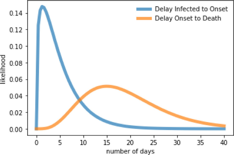
The delay to isolation (or onset of symptoms) d_iso and delay to death from isolation $d_{iso-death}$ distributions that are used in this study are illustrated in Fig. 2 .

Fig. 2.

Illustration of probability density functions for d_iso and $d_{iso-death}$ used in the current study. The parameters of the distributions are used from [11].

P _d(t): probability that a person infected with the Covid-19 virus will die. This is commonly referred to as the mortality rate of the disease or the case-to-fatality rate. The mortality rate (death rate / case-fatality ratio) can be considered fixed when the healthcare capacity is not reached in a given region. The current values reported in literature varies significantly from around 0.001 to 0.12, with a bias towards lower estimates. In our experiments, we used death rates (Case-fatality ratio) of 0.0025, 0.03 and 0.1.

t _fd: the first day that new deaths reported is >10.

2.1. Estimation of number of cases infected in a day

Based on the delay to death distribution d_death, the minimum death delay (min [d_death]) and maximum death delay (max [d_death]) are assumed to be the 1% quantile and 95% quantile of d_death respectively. The expected deaths for the t^th day, denoted as E[D(t)] for t ≥ max [d_death] can be calculated by

$$E\left[D\left(t\right)\right]=\begin{array}{c}\sum _{i=t-\max \left[d_{death}\right]+1}^{t-\min \left[d_{death}\right]}{P}_d\left(i\right)·N\left(i\right)·\mathrm{Pr}\left(t-i<d_{death}\le t-i+1\right)\end{array}$$ (1)

In matrix form this corresponds to:

$$\overrightarrow{E}\left[D\left(t\right)\right]=M·\overrightarrow{N}\left(t\right)$$ (2)

Where M is made up of Pd and Pr values of Eq. (1).

The above equation suggests that, of those who contract the virus on a day i, a certain fraction P _d(i), eventually die after a delay of several days. The delay is governed by the distribution d _death.

To further explain the application of equation Eq. (2), we assume that $\min \left[d_{death}\right]=7$, $\max \left[d_{death}\right]=41$, and the daily death data is available from 41st day to 103rd day. Using the equation above, $\overrightarrow{E}\left[D\left(t\right)\right]$ is a vector of length 63, M is a 63 × 96 matrix and $\overrightarrow{N}\left(t\right)$ is a vector of length 96. E[D(t)] for $t=41,\dots ,103$ can be calculated by:

$$\begin{array}{ccc}\hfill E\left[D\left(41\right)\right]& =& p_d\left(1\right)·N\left(1\right)·P\left(41\right)+p_d\left(2\right)·N\left(2\right)·P\left(40\right)\hfill \\ & & +\cdots +p_d\left(34\right)·N\left(34\right)·P\left(8\right)\hfill \\ \hfill E\left[D\left(42\right)\right]& =& p_d\left(2\right)·N\left(2\right)·P\left(41\right)+p_d\left(3\right)·N\left(3\right)·P\left(40\right)\hfill \\ & & +\cdots +p_d\left(35\right)·N\left(35\right)·P\left(8\right)\hfill \\ & & ⋮\hfill \\ \hfill E\left[D\left(103\right)\right]& =& p_d\left(63\right)·N\left(63\right)·P\left(41\right)+p_d\left(64\right)·N\left(64\right)·P\left(40\right)\hfill \\ & & +\cdots +p_d\left(96\right)·N\left(96\right)·P\left(8\right)\hfill \end{array}$$

Given deaths data D(t) for $t=t_1,\dots ,t_{current}$, the estimation of daily new infection $\tilde{N}\left(t\right)$ for $t=t_1-\max \left[d_{death}\right]+1,\dots ,t_{current}-\min \left[d_{death}\right]$ can be found by minimizing the difference between model prediction E[D(t)] and the real daily death numbers D(t):

$$\tilde{N}=arg\underset{\tilde{N}}{min}{\left(E\left[D\left(t\right)\right]-D\left(t\right)\right)}^2$$ (3)

This is a quadratic optimization problem, which can be solved by using Quadratic Programming [12]. In our model, a linearly constrained Quadratic Programming was used to find the estimation of daily new infection. To get a realistic estimation, several linear constraints for $\tilde{N}\left(t\right)$ were added to the model, including boundaries for the ratio $\tilde{N}\left(t+1\right)/\tilde{N}\left(t\right)$, the ratio $\tilde{N}\left(t+m\right)/\tilde{N}\left(t\right)$ and cumulative growth rate $N_{cum}\left(t+1\right)/N_{cum}\left(t\right)$ for each day.

Ideally, adding constraints on the dynamic of growth rate could help us find $\tilde{N}\left(t\right)$ with less oscillation and smoother in the long term. Therefore, none-convex quadratically constrained Quadratic Programming could potentially improve our estimation of daily new infection.

2.2. Calculation of effective reproduction number

The expected value of effective reproduction number for the day t, denoted by E[R(t)], is estimated by the following equation:

$$E\left[R\left(t\right)\right]=\mathit{No}.\mathit{of}\mathit{Cases}\mathit{Infe}\mathit{cted}\mathit{by}N\left(t\right)/N\left(t\right)$$ (4)

The R estimation in the method is performed daily according to the Eq. (4). The calculation of the numerator on Eq. (4) is not straightforward. The newly infected patients on day t, denoted by N(t) in the denominator of Eq. (4), will be continuously infectious on future days until they are isolated or recovered. Consequently, the number of newly infected cases on a given future date, would have been infected by all the people who are infectious on the previous days. However, the people who are infectious on the previous days, were first infected on different days in the past. Therefore, the method should consider the proportion of people who are exclusively infected by those who were first infected on a given date (N(t)).

For this purpose, it is required to calculate the number of people infected in the previous days, and also account for those of whom are no longer infectious due to self-isolation/hospitalization or recovery.

The following paragraphs explain how this is calculated.

Assuming N(t) is available for $t=1,..,n$, we define $\overrightarrow{N_0}=[N\left(1\right),\cdots ,N(n-1)]$ and $\overrightarrow{N}=[N\left(2\right),\cdots ,N\left(n\right)]$.

The cumulative Infections matrix I, is defined to collate the number of infectious cases on day $i+1$, who were infected on the previous days. I is a lower triangular matrix of size $n-1$ x $n-1$, where I[i, j] is the number of infectious cases on day $i+1$, who were first infected on day j. We assumed that each infected case becomes infectious on the next day.

$$I[i,i]=N\left(i\right)\mathit{f}\mathit{or}i=1,\cdots ,n-1$$ (5)

The rows of column j of the matrix I is defined by spreading the infectious cases first infected on day j by using the gamma distribution representing the d_iso.

The process for finding the values for I[i, j], where  i > j is as follows.

For each $j=1,\dots ,n-1$, sample from d_iso for N(j) times. The samples from d_iso are denoted by $S=\left(s_1,s_2,\dots ..,s_{N\left(j\right)}\right)$.

$$s_k\sim \Gamma \left(\alpha =1.35,\beta =\frac{1}{0.27}\right)$$ (6)

where α is the shape parameter, and the β is the scale parameter of the gamma distribution.

If a sample s_k from S is $m-1<s_k<m$, this indicates that it took m days for this infected case to isolate.

$$I\left[i,j\right]=I\left[j,j\right]-S{C}_{i-j}$$ (7)

Where SC_ris the number of $s_k\in S,suchthatr-1<s_k<r$

The above sampling process is evaluated for 100 times and the average I is considered to calculate the effective reproduction number.

From the cumulative infectious matrix I, a weighting matrix W is defined as below, where each element of the matrix W, W[i, j] is defined as:

$$W\left[i,j\right]=\frac{I\left[i,j\right]}{{\sum }_{k=1}^{n-1}I\left[i,k\right]}$$ (8)

$$E\left[R\right]=\frac{\overrightarrow{N}·W}{\overrightarrow{N_0}}$$ (9)

The E[R] is a $1\times \left(n-1\right)$ array, representing the approximated effective reproduction number on days 1 to ($n-1$). The estimated effective reproduction number is denoted as R in the proceeding discussions.

A Python implementation of the methodology is provided through GitHub (https://github.com/JJJJJamie/r_estimation).

3. Experimental results

The results section is mainly organised in two parts. Firstly, proposed model is validated against an SIR simulation and secondly, we present results for reproduction number predictions for 2 selected countries.

3.1. Model validation

For the purpose of model validation, we simulate a disease outbreak with an SIR model [13], to estimate the number of infected populations under a varying R value over time. A certain fraction of the infected population is simulated to die. Those who die, will die after a certain number of days, and this number of days of delay to death from the moment of removed (isolation) is governed by the distribution $d_{iso-death}$. The parameters of $d_{iso-death}$ are defined same as in section 2.

The objective of this experiment is to validate the proposed probabilistic model. The proposed methodology utilizes the daily death data D(t), to estimate the number of infected cases N(t). Then estimates the R(t) from the estimated N(t). We assume we have perfect knowledge of the delay to death distribution, hence use the same parameters as the simulation, for R(t) estimation. The sensitivity of this assumption is analysed in the proceeding subsection.

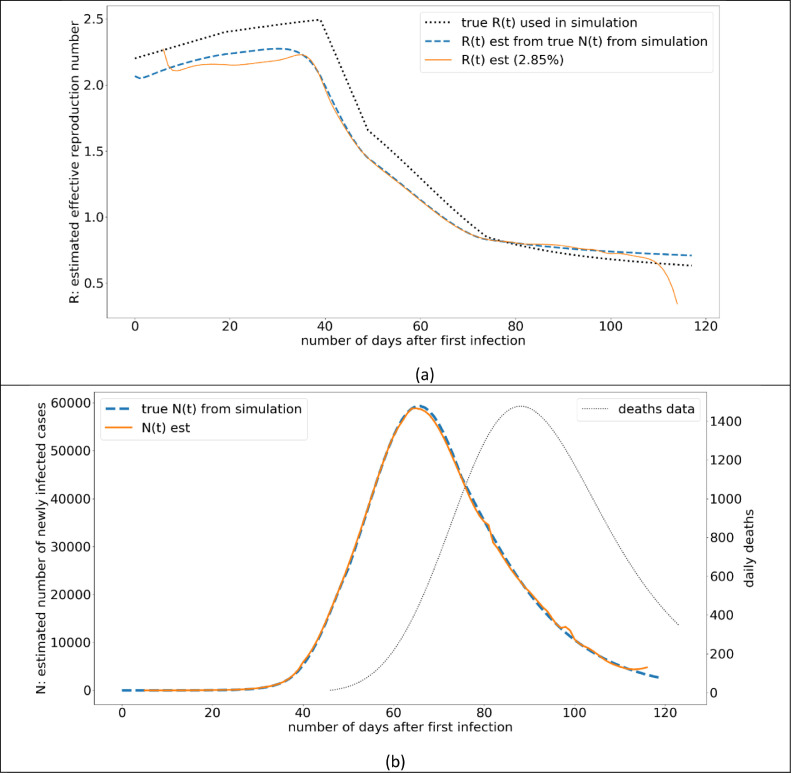
The results of this experiment are illustrated in Fig. 3 . In Fig. 3(b), the simulated death data and the number of infections are illustrated. Estimation of N(t) from death data is an important part of the proposed method (As in the case of COVID-19 this is an unknown because not everyone in the population is tested, nor everyone shows symptoms when infected). The N(t) values from the model, closely agrees with the true N(t) values (from simulation). The R(t) estimation from N(t) is illustrated in Fig. 3(a). The estimated R(t) follows a similar pattern to the true R(t) that is simulated, however, there is a consistent under estimation of around 0.25 points of R. Furthermore, the R(t) estimation, when done utilizing the true N(t) values from the simulation, agrees very much with overall model.

Fig. 3.

Model Validation: (a) The variation of simulated R(t) value, and the R(t) value estimated from the proposed model, (b).

3.2. Sensitivity analysis

The sensitivity of the model is assessed across 3 attributes of the proposed model: the distribution of delay to death from removed (isolation), the mortality rate and the noise level on the death statistics. Furthermore, since the proposed model is dependent on the delay to death, we also assess the ability of the model to estimate the R, in the case of limited death data.

3.2.1. Model predictions under different death delay distributions

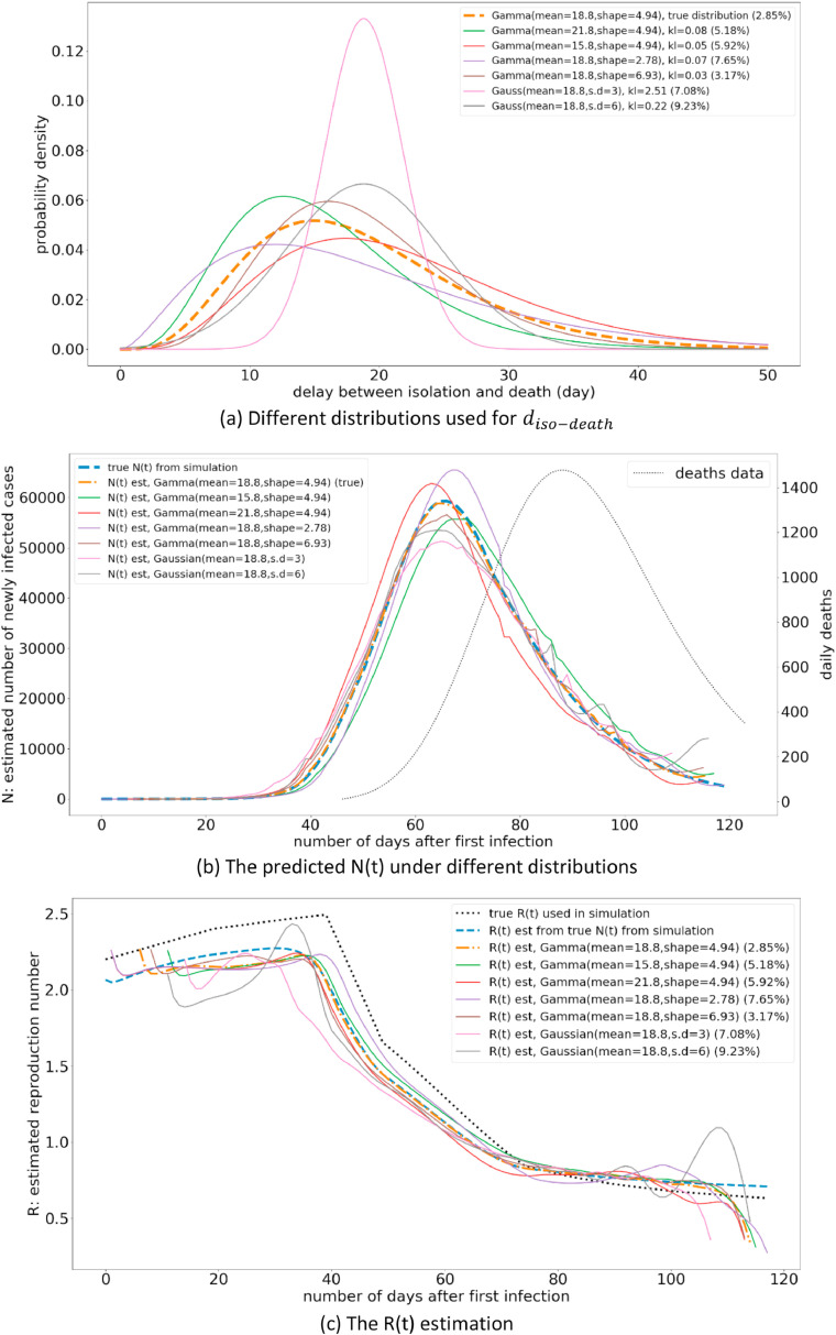
In Section 3.1, we assumed the perfect knowledge of the $d_{iso-death}$distribution. However, this is a very unlikely assumption, and the knowledge of this distribution would not be available until a country has gone through an adequate period of the pandemic. Therefore, this experiment analyses the sensitivity of the prediction from the proposed model under different $d_{iso-death}$distributions that will be used for R(t) estimation. For the purpose of this experiment, we utilize the KL-divergence to quantify the difference between two probability distributions. The results of this experiment are illustrated in Fig. 4 .

Fig. 4.

The variation of R(t) estimation under different $d_{iso-death}$ distributions.

The results in Fig. 4 illustrate that the model estimates show a similar trend regardless of the investigated distributions. Furthermore, the estimated R value is mostly within 0.25 of the true R value, when the distribution is a gamma distribution. However, when the distribution used in the model is a Gaussian distribution, the error is much larger compared to when using a gamma distribution.

3.2.2. Model predictions under different mortality rates and death report rates

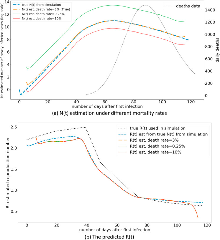
The mortality rate of the disease denoted by P_d is utilized for the estimation of R(t) in the proposed methodology. While this would not be known until the end of the pandemic, there are initial estimates of this important parameter. The Fig. 5 illustrates the model performance under different mortality rates.

Fig. 5.

The variation of R(t) estimation under different mortality rates (Pd).

The results indicate that, although the mortality rate affects the number of infected cases in the population (N(t)), it does not affect the R estimation. This is an important property to enable robust R estimations when different countries under-report deaths due to variations in the counting criteria. In such a case where the deaths are under-reported, the R estimation from the proposed method is not affected, as long as the death reporting mechanism stays consistent throughout the period of R-estimation. If the death reporting mechanism changes over the period of the pandemic for a given country, this should be incorporated within the model.

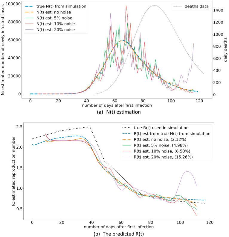
3.2.3. Model predictions under different noise levels on the death statistics

Another issue associated with using the daily death statistics is that the death curve is not always smooth, and there are daily variations. The Fig. 6 illustrate the effect of noise on the daily death statistics on the final R estimation. The results illustrate that unless there is a significant amount of noise on the daily death statistics (e.g. 20%), the R estimation is not significantly affected.

Fig. 6.

The variation of R(t) estimation under different noise levels on the death statistics.

3.2.4. On the gap between death data availability and accuracy of the R estimation

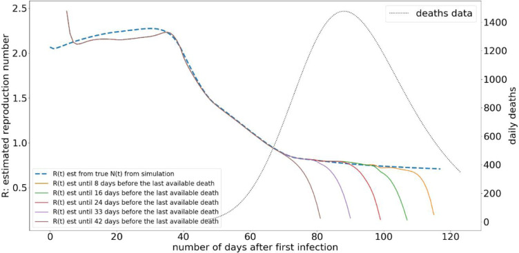
The complete death data is available for a disease, only after the end of a pandemic. However, in the case of a pandemic such as COVID-19, where governments have to consistently take suppression measures during the pandemic, the ability to estimate R during the pandemic is extremely important as a measure of disease spread. The proposed model uses the daily death statistics for estimation of R(t), and due to the dynamics of the disease there is a delay to death of an infected person. Therefore, there is a gap when R value can be estimated with a reasonable accuracy, and the most recent availability of death statistics.

We illustrate the variation of R(t) estimation under different gaps between the most recent death data availability and the R(t) estimation, in Fig. 7 . According to Fig. 7 the R estimation does not change very much, if we have the perfect knowledge of the underlying d_death distribution and when there is no noise on the death data. It should be noted that due to the lack of complete N(t) estimations from the available death data, the curve will always bend towards the end.

Fig. 7.

The variation of R(t) estimation under different gaps from the most recent death data availability. The “true” delay from isolation to death is simulated as a gamma distribution with mean = 18.8, and shape = 4.94, and same distribution used in the method.

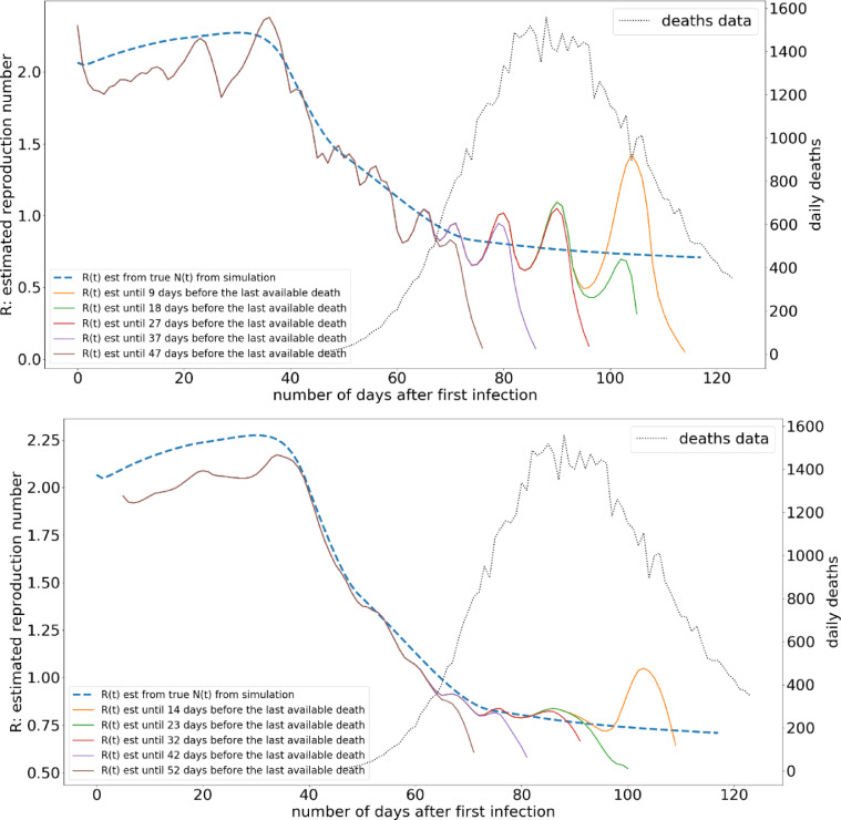
The effect under a different distribution and under noise is illustrated in Fig. 8 , which suggests that R estimation will be affected by these changes. However, the variation of R estimation is still largely preserved, and the oscillations on the R estimation can easily overcome through a smoothing operation.

Fig. 8.

The variation of R(t) estimation under different gaps from the most recent death data availability. The delay from isolation to death is “assumed” as a gamma distribution with mean = 21.8, and shape = 4.94, the noise level on the death data is 5%.

3.3. Application of model for different countries

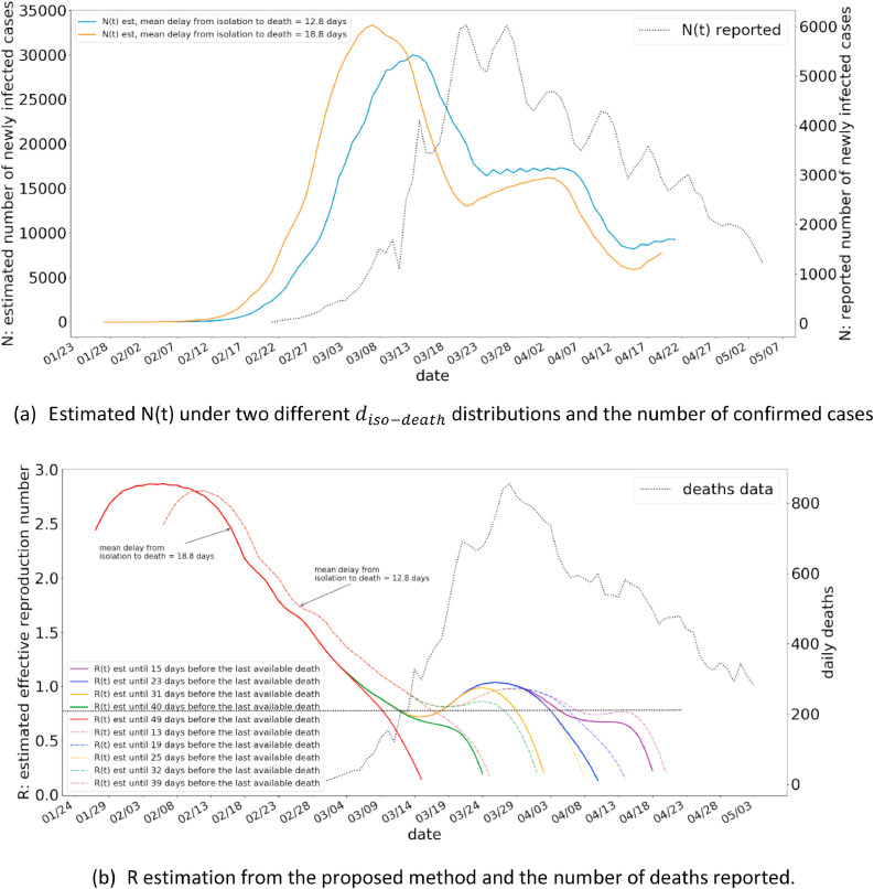
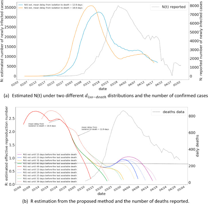
In this subsection we present the R-estimation results for two different countries, using the proposed method. We have selected Italy and Spain, the countries which have nearly progressed through the pandemic. We have used the most up to date death statistics (as of writing of this paper) for this purpose. The results are presented in Fig. 9 for Italy, and Fig. 10 for Spain.

Fig. 9.

The R estimations for Italy from the proposed method.

Fig. 10.

The R estimations for Italy from the proposed method.

The Fig. 9(a) illustrates the estimated N(t) under different distribution of $d_{iso-death}$, along with the number of confirmed cases in Italy. As illustrated, gamma distribution with a mean of 12.8 days closely agrees with the shape of the number of reported cases, and also exhibits a shift of around 10 to 14 days to be in line with a delay associated with being reported due to intensifying symptoms. The R estimations from the method shows a peak R value of 2.8 to a gradually decreasing R value. The current R value in Italy is estimated from the method to be between 0.5 and 1. A similar pattern is also observed for Spain.

4. Discussion

The aim of this paper is to utilize the publicly available data to measure the spread of disease by calculating the effective reproduction number of the disease, especially during the pandemic. During the early stages of a pandemic, only a limited amount of data is made available. However, knowing the reproduction number throughout the pandemic is of significant essence to make public health decisions. In the current pandemic of COVID-19, the number of confirmed cases and the number of deaths is reported by most countries. However, the number of confirmed cases is significantly dependent on the testing strategy employed by public health bodies of a country, and cannot be used as a useful statistic of the underlying number of infectious people. Therefore, at early stages of a pandemic, the methodology uses the daily deaths as the only statistic and work backwards to calculate the effective reproduction number.

4.1. Performance of the model

The performance of the proposed probabilistic model is estimated through simulations for validation purposes. The results presented in Section 3.2, suggests that the proposed method is robust against variations in delay to death distribution and the noise level in death statistics. It should also be noted that, when death data is available up to a given date, the model can accurately predict R up to around 40 days before depending on the accuracy of assumed death delay distribution and the noise level of death data. This is mostly stemming from the fact that deaths are delayed by a significant number of days from the date of first infection. However, as illustrated in Figs. 7 and 8 the R can be estimated for up to 14 days before the last date for which death data is available, with a reasonable accuracy. The R estimation, however, tends to oscillate between 40 days and 14 days, which can be overcome through smoothing as shown in Fig. 8.

Most importantly, R estimation from this method is not affected by the mortality rate (or death rate) assumed for the disease. This is illustrated in Fig. 5. The implications of results in Fig. 5, also relates to the death report rate variation across countries. This is because, variation in death rate simulations is synonymous with the different death report rates too. Different countries count the number of deaths with different logics, E.g. some countries may count only the deaths of those with confirmed positive test for COVID-19 who die only in hospitals but disregard the deaths in care homes. However, as long as the counting logic is consistent, throughout the reporting period, the death report rate will be constant, and thus enabling the estimation R, which is not affected by the death rate (or death report rate).

The methodology utilizes existing studies about the delay between infection and onset of symptoms and the delay between onset of symptoms and death. However, these studies are still emerging and show significant variations among the distributions used [14], but has a strong correlation on the mean values.

4.2. Applications of the model for COVID-19 analysis in different countries

The results in Figs. 9 and 10 demonstrate the model performance on real death statistics from Italy and Spain, respectively. A suitable delay to death distribution was found by trying to match a N(t) estimation that is similar in variation, but which is shifted by a certain reporting delay (Figs. 9(a) and 10(a)). The R estimation for Italy and Spain has been gradually decreasing during months of March and April and is currently (at the time of writing the paper) stable at a value between 0.5 and 1, with a mean estimation of around 0.8. The starting level of R, for both Italy and Spain was around 2.7 (i.e. before any suppression measure was taken). This estimation is in consistent with the initial estimates of R provided in [15], which suggested for Italy the mean R value was 2.3, and for Spain it was 3.11.

The R value is one of the most important metrics of the spread of infectious diseases. The knowledge of R enables public health authorities to make important decisions such as implementation of suppression policies, and appropriate timing of such policies. For example, in the control of COVID-19 spread, most countries have implemented suppression mechanisms such as school closures, travel bans and lockdowns. The correct timing of such measures is of utmost importance, and the knowledge of the level of spread of the disease is the most important criteria to implement the stringent measures, and for the subsequent easing of such suppression methods. The availability of an alternative model such as the proposed, will assist the epidemiologists and policy makers to understand the spread of the disease, as well as a sanity check mechanism on the estimations of R values based on SIR models.

Another important application of the proposed methodology is the ability of it to predict number of infectious people in a given country (N(t)). This is particularly important for the case of COVID-19, because a significant proportion of those who are infected are asymptotic.

4.3. Challenges of practical application of the model for COVID-19 analysis

The proposed methodology is dependent on the number of deaths reported and made public. However, in the case of COVID-19 and the deaths are delayed according to d_death. Therefore, to calculate the N(t) at current date, the number of deaths of the future day needs to be predicted. In the case of COVID-19, a person can die up to 42 days from the onset of symptoms (95% Confidence Interval). However, predicting the future deaths of a given country is a very challenging task. This is because, the number of deaths is dependent on many factors such as, the suppression policies employed in the country and the healthcare capacity. Therefore, to calculate the most up-to-date R we would need a suitable machine learning model to predict the deaths in the future. State-of-the-art machine learning techniques could significantly contribute to this task.

The proposed methodology assumes a base mortality rate for the purpose of estimation of R. We present the results for three values of mortality rates, 0.0025, 0.03, (consistent with different studies [16,17]) and 0.1 as an extreme case. However, when the pandemic causes the healthcare resources to be exhausted, the mortality rate can be expected to be higher, such as 0.12 [18]. Therefore, the variation of mortality rate within the period of pandemic need to be quantified to be used within the model. This again is an important, yet challenging research problem that need to be solved.

Another important consideration is, that different countries have different methods of counting the number of COVID-19 related deaths. For example, until 29th of April, the UK government considered COVID-19 related deaths that happen only in Hospitals, to then change their policy to include deaths in care homes too. Such a change in policy causes the number of deaths reported to significantly vary with time. While this can easily be adopted within the proposed model by a simple change in the death rate, calculating the dynamic death report rate of a country can be challenging. This is especially a problem during the early stages of a pandemic when the government policies are rapidly changing.

5.Conclusion

This paper presents a probabilistic methodology to estimate the effective reproduction number (R) of a given country, using the daily statistics of death. The methodology utilizes existing studies on COVID-19 related to the probability distributions of the delay between infection and onset of symptoms, and the delay between onset of symptoms and death. The proposed methodology is validated by comparing against simulated disease spread using a SIR simulation. The R-estimates from the proposed method was found to be robust against different distributions of delay to death from the onset of symptoms, and against different noise levels on the death statistics. The R estimates from the proposed method is shown to be constant against different death report rates or mortality rate of the disease, and the model can be useful up to 14 days before the last available death data. The R-estimates of the model for Italy and Spain shows a consistent pattern and agrees with estimates from emerging studies. The proposed method is useful to calculatethe effective reproduction number. Most importantly, since scientists are still learning the dynamics of the virus, a methodology that is proposed here provides a useful model for informing policy decisions. Furthermore, a data-driven methodology can be an alternative avenue to analytical model driven approaches for estimation of R, thus serving as an additional analysis tool to study the spread of COVID-19.

Declaration of Competing Interest

Please check the following as appropriate:

• •All authors have participated in (a) conception and design, or analysis and interpretation of the data; (b) drafting the article or revising it critically for important intellectual content; and (c) approval of the final version.
• •This manuscript has not been submitted to, nor is under review at, another journal or other publishing venue.

References

- 1.Dietz K. The estimation of the basic reproduction number for infectious diseases. Stat Methods Med Res. 1993;2:23–41. doi: 10.1177/096228029300200103. [DOI] [PubMed] [Google Scholar]
- 2.Ridenhour B., Kowalik J.M., Shay D.K. Unraveling R0: considerations for Public Health Applications. Am J Public Health. 2014;104:e32–e41. doi: 10.2105/AJPH.2013.301704. [DOI] [PMC free article] [PubMed] [Google Scholar]
- 3.Park M., Cook A.R., Lim J.T., Sun Y., Dickens B.L. A Systematic Review of COVID-19 Epidemiology Based on Current Evidence. J Clin Med. 2020;9:967. doi: 10.3390/jcm9040967. [DOI] [PMC free article] [PubMed] [Google Scholar]
- 4.Kucharski A.J., Russell T.W., Diamond C., Liu Y., Edmunds J., Funk S. Early dynamics of transmission and control of COVID-19: a mathematical modelling study. The Lancet Infect Dis. 2020;0 doi: 10.1016/S1473-3099(20)30144-4. [DOI] [PMC free article] [PubMed] [Google Scholar]
- 5.Lin Q., Zhao S., Gao D., Lou Y., Yang S., Musa S.S. A conceptual model for the coronavirus disease 2019 (COVID-19) outbreak in Wuhan, China with individual reaction and governmental action. Int J Infect Dis. 2020;93:211–216. doi: 10.1016/j.ijid.2020.02.058. [DOI] [PMC free article] [PubMed] [Google Scholar]
- 6.Zhang S., Diao M., Yu W., Pei L., Lin Z., Chen D. Estimation of the reproductive number of novel coronavirus (COVID-19) and the probable outbreak size on the Diamond Princess cruise ship: a data-driven analysis. Int J Infect Dis. 2020;93:201–204. doi: 10.1016/j.ijid.2020.02.033. [DOI] [PMC free article] [PubMed] [Google Scholar]
- 7.Ivorra B., Ferrández M.R., Vela-Pérez M., Ramos A.M. Mathematical modeling of the spread of the coronavirus disease 2019 (COVID-19) taking into account the undetected infections. The case of China. Commun Nonlinear Sci Numer Simul. 2020 doi: 10.1016/j.cnsns.2020.105303. [DOI] [PMC free article] [PubMed] [Google Scholar]
- 8.Diekmann O., Heesterbeek J.a.P., Roberts M.G. The construction of next-generation matrices for compartmental epidemic models. J R Soc Interface. 2010;7:873–885. doi: 10.1098/rsif.2009.0386. [DOI] [PMC free article] [PubMed] [Google Scholar]
- 9.de-Camino-Beck T., Lewis M.A., van den Driessche P. A graph-theoretic method for the basic reproduction number in continuous time epidemiological models. J Math Biol. 2009;59:503–516. doi: 10.1007/s00285-008-0240-9. [DOI] [PubMed] [Google Scholar]
- 10.Mills C.E., Robins J.M., Lipsitch M. Transmissibility of 1918 pandemic influenza. Nature. 2004;432:904–906. doi: 10.1038/nature03063. [DOI] [PMC free article] [PubMed] [Google Scholar]
- 11.Flaxman S., Mishra S., Gandy A., Unwin H.J.T., Coupland H., Mellan T.A., Berah T., Eaton J.W., Guzman P.N.P., Schmit N.;. Estimating the number of infections and the impact of non- pharmaceutical interventions on COVID-19 in 11 European countries. Imperial College COVID-19 Response Team. 2020:35. [Google Scholar]
- 12.Jensen P, Bard J, Quadratic Programming. Oper Res Model Methods5.
- 13.Brauer F. Compartmental Models in Epidemiology. In Mathematical Epidemiology. In: Brauer F., van den Driessche P., Wu J., editors. Lecture notes in mathematics. Springer: Berlin; Heidelberg: 2008. pp. 19–79. ISBN 978-3-540-78911-6. [Google Scholar]
- 14.Linton N.M., Kobayashi T., Yang Y., Hayashi K., Akhmetzhanov A.R., Jung S. Incubation Period and Other Epidemiological Characteristics of 2019 Novel Coronavirus Infections with Right Truncation: a Statistical Analysis of Publicly Available Case Data. J Clin Med. 2020;9:538. doi: 10.3390/jcm9020538. [DOI] [PMC free article] [PubMed] [Google Scholar]
- 15.Yuan J., Li M., Lv G., Lu Z.K. Monitoring Transmissibility and Mortality of COVID-19 in Europe. Int J Infect Dis. 2020;0 doi: 10.1016/j.ijid.2020.03.050. [DOI] [PMC free article] [PubMed] [Google Scholar]
- 16.Wilson N., Kvalsvig A., Barnard L.T., Baker M.G. Early Release - Case-Fatality Risk Estimates for COVID-19 Calculated by Using a Lag Time for Fatality. Emerg Infect Dis J. 2020;(26) doi: 10.3201/eid2606.200320. [DOI] [PMC free article] [PubMed] [Google Scholar]
- 17.Verity R., Okell L.C., Dorigatti I., Winskill P., Whittaker C., Imai N. Estimates of the severity of coronavirus disease 2019: a model-based analysis. The Lancet Infect Dis. 2020 doi: 10.1016/S1473-3099(20)30243-7. [DOI] [PMC free article] [PubMed] [Google Scholar]
- 18.Mizumoto K., Chowell G. Early Release - Estimating Risk for Death from 2019 Novel Coronavirus Disease, China. Emerg Infect Dis. 2020;26 doi: 10.3201/eid2606.200233. January–February 2020. [DOI] [PMC free article] [PubMed] [Google Scholar]