Identification of an α-MoRF in the Intrinsically Disordered Region of the Escargot Transcription Factor

Abstract

Molecular recognition features (MoRFs) are common in intrinsically disordered proteins (IDPs) and intrinsically disordered regions (IDRs). MoRFs are in constant order–disorder structural transitions and adopt well-defined structures once they are bound to their targets. Here, we study Escargot (Esg), a transcription factor in Drosophila melanogaster that regulates multiple cellular functions, and consists of a disordered N-terminal domain and a group of zinc fingers at its C-terminal domain. We analyzed the N-terminal domain of Esg with disorder predictors and identified a region of 45 amino acids with high probability to form ordered structures, which we named S2. Through 54 μs of molecular dynamics (MD) simulations using CHARMM36 and implicit solvent (generalized Born/surface area (GBSA)), we characterized the conformational landscape of S2 and found an α-MoRF of ∼16 amino acids stabilized by key contacts within the helix. To test the importance of these contacts in the stability of the α-MoRF, we evaluated the effect of point mutations that would impair these interactions, running 24 μs of MD for each mutation. The mutations had mild effects on the MoRF, and in some cases, led to gain of residual structure through long-range contacts of the α-MoRF and the rest of the S2 region. As this could be an effect of the force field and solvent model we used, we benchmarked our simulation protocol by carrying out 32 μs of MD for the (AAQAA)₃ peptide. The results of the benchmark indicate that the global amount of helix in shorter peptides like (AAQAA)₃ is reasonably predicted. Careful analysis of the runs of S2 and its mutants suggests that the mutation to hydrophobic residues may have nucleated long-range hydrophobic and aromatic interactions that stabilize the MoRF. Finally, we have identified a set of residues that stabilize an α-MoRF in a region still without functional annotations in Esg.

1. Introduction

Intrinsically disordered proteins (IDPs) or intrinsically disordered regions (IDRs) have no stable, well-defined three-dimensional structures under physiological conditions. They play an important role in many biological functions, such as organ development, and their dysfunction is associated with multiple diseases.¹⁻³ One of the main goals of studying IDPs is to understand their capacity to adopt multiple conformations and to explore the binding mechanisms leading to interactions and their biological functions.

For those IDPs that fold upon binding, this has been analyzed in terms of two extreme models: “conformational selection” and “induced fit”.⁴ In the conformational selection mechanism, the protein explores conformations that are both ordered and disordered, and specific folded conformations are selected by the ligand; in the induced fit mechanism, the conformational change occurs after the disordered protein is bound to the ligand^4,5 and this process is known as “template folding”, where the folding transition state is dictated by the interactions with the ligand.⁶ Real cases present a mixture of these two scenarios.

Residual structure often persists in unbound IDPs.⁷⁻⁹ These preformed but unstable structural elements might serve as initial contact points to facilitate the folding and recognition of the ligand surface.⁷⁻¹⁰ These residual structures may exist in short regions known as molecular recognition features (MoRFs), which can be found in long disordered regions of IDPs and IDRs.^11,12 MoRFs are mainly disordered in their unbound states and adopt local structures that are stabilized when they interact with their targets.¹¹ MoRFs are classified according to their structures in the bound state, where α-MoRFs form α-helices, β-MoRFs form β-strands, ι-MoRFs form irregular structures (coil conformations), and complex MoRFs adopt a conformation resulting from the combination of the other types.^13,14 MoRFs play important roles in signaling and regulatory functions,^12,15 and transcription factors are enriched in IDRs.^16,17

Exploring and characterizing the conformational ensemble of IDPs is not an easy task, as they are represented by multiple conformations, and different ones can be associated with particular functions. Many experimental techniques, such as dynamic light scattering, small-angle X-ray scattering, paramagnetic relaxation enhancement, and circular dichroism, are useful to obtain information on the ensemble-average of diverse conformations of IDPs. Computational techniques are also used; for example, molecular dynamics (MD) and Monte Carlo (MC) simulations have been useful to complement the information obtained by experimental techniques and to characterize the conformational ensembles at the atomic level.^1,2,18,19

Simulations allow us to study the molecular features and motions of IDPs. However, structural characterization by simulations is limited by the long time required for adequate conformational sampling and by the accuracy of the parameters of the force fields and the explicit or implicit solvent models used. Protein force fields were developed and parameterized mainly to describe folded proteins^2,20 and their application has been thoroughly benchmarked, but their applicability to IDPs requires considerable attention and continuous improvement;^1,19 different force fields and protocols with explicit and implicit solvent models have been applied to various IDPs (summarized in Table S1 for the past 5 years).

The motions of conformational changes in an IDP happen in time scales spanning several orders of magnitude (between picosecond (ps) to microsecond (ms))²¹ and this implies substantial computational costs, depending on the system size.²² The behavior of protein chains in solution depends fundamentally on the balance of solute–solute versus solute–solvent and solvent–solvent interactions.²³ The effects of the solvent environment can be treated using explicit or implicit solvent representations.^8,23 Explicit solvents treat both protein and water molecules explicitly, significantly increasing the system size (∼10 fold) and leading to large computer requirements²⁴ in simulations of protein folding^8,23,25 or characterization of the conformational ensembles of IDPs.²⁵ This approach has been successful in reproducing and explaining experimental measurements.^3,26−29 Alternatively, implicit solvent models are popular because they include explicitly only the atomic coordinates of the protein, as the water molecules are represented by an infinite continuum medium with the macroscopic properties of water; this reduces the computational cost and allows for longer simulation times required for simulating conformational transitions, especially in novo simulations of IDPs.^7,23,24,30 Modeling small IDPs with an implicit solvent has also been successful.^{23,25,31−33}

However, both explicit and implicit solvent models have limitations. For example, some combinations of force fields and water models such as TIP3P, TIP4P, and TIP4P-EW generate overly compact conformational IDP ensembles.^2,34,35 As some IDPs are enriched in charged and polar residues,^1,36 their structural properties make them sensitive to interactions with water.² This effect of overcompaction could be the result of underestimating water–water and water–protein interactions³⁴ or a mismatch between the protein force field and the water model.³⁵ For this reason, it is paramount to validate the combination of the force field and water model used.²⁰ On the other hand, many implicit solvent models also tend to generate conformations that are too structured and compact.^22,37 There are important structural properties of water and short-range effects that are not considered in implicit solvent models, and their disregard can lead to different folding mechanisms.^38,39 Optimization efforts have also led to improvements in the implicit solvent models,²³ such as the ABSINTH implicit solvent force field that was developed and optimized specifically for IDPs.^8,31

Some of the force fields generate more compact conformations than others, as well as overstabilization of specific conformations.²⁰ Nowadays, there is no standard, specific protocol to simulate IDPs, but there is a continuous search for developing and improving force fields and sampling strategies that can be applied to both folded proteins and IDPs.¹⁹ As can be seen from the simulations listed in Table S1, both MD and MC simulations are useful, and enhanced sampling techniques such as replica exchange (the temperature and the Hamiltonian versions) have also been used. Given the vastness of the conformational space to the sample, another strategy is to guide the simulations with experimental data or to reweigh the simulated ensemble to approximate the experimental data. These procedures only work for original ensembles that are close to the target, so the quality of the force fields and sampling must be good. Fortunately, significant progress has recently been made in the ability of MD force fields to accurately describe folded proteins and IDPs.⁴⁰⁻⁴³ Central to this progress is having small benchmark systems that are well characterized experimentally, such as the 15-residue (AAQAA)₃ peptide that has been used for studying protein folding, characterize the helix–coil transitions, and to parameterize and validate different force fields^{21,38,39,41,42} (summarized in Table S2).

Here, we study the N-terminal disordered domain of Escargot (Esg), a transcription factor of the Snail family, to look for potential MoRFs associated with Esg functions that are independent of its DNA-binding activity. We performed MD simulations starting from semifolded structures to characterize the conformational ensemble of a region with high propensity to order, using CHARMM36 and an implicit solvent model (generalized Born model, or generalized Born/surface area (GBSA)). Having identified a probable residual structure that adopts α-MoRF conformations and detailed the interactions that stabilize it, we proposed mutations that would destabilize it and simulated them as well. Contrary to our expectations, the mutations did not lead to dramatic losses of structure. Careful analysis of the inherent bias of our simulation protocol and of the interactions that stabilize the residual structure in the mutants revealed a network of hydrophobic and aromatic interactions stabilizing the α-MoRF. This allows us to propose a set of critical residues for the formation and stability of this α-MoRF; these could be tested by mutagenesis experimentally, to determine the functional role of this region of Esg, which lacks annotated functional motifs. Our results might also be helpful as a benchmark for this combination of a force field and a solvent model, aiding in future refinements of both. This is the first structural analysis of the N-terminal region of Esg and aims to foster future studies into the structure–function relationship of this region to understand the mechanism of regulation of this transcription factor.

2. Results and Discussion

Esg is a protein of 470 residues, which is expressed in Drosophila melanogaster, and is involved in the development of the nervous system.^44,45 Structurally, the Esg C-terminal domain (CTD) is a conserved region that has five classical zinc fingers (ZNFs) and interacts with nucleic acids,⁴⁶ while the N-terminal domain is divergent,^45,46 and the only functional annotation in this region consists of two motifs (P-DLS-K) that interact with the C-terminal binding protein (CtBP),⁴⁷ a transcriptional repressor. However, the N-terminal domain (NTD) has been associated with functions such as protein degradation, where the ZNFs are not necessary,⁴⁴ but the actual functional motifs for this and other activities have not been described.

2.1. The NTD of Esg is an IDR

Using four disorder predictor programs and averaging the output scores of all of the predictors, we generated a profile of disorder (Figure 1) that reveals that the NTD is highly disordered, in contrast to the CTD (residues 310–470) containing the ZNFs. The disorder profile of the NTD was split into three regions: S1 (residues 1–110), S2 (residues 111–155), and S3 (residues 156–309), where the S2 region has a much higher probability to adopt order than the other two.

Figure 1.

Disorder probability analysis of the Esg protein. The plot shows the average probability of disorder by residue. The light and dark green color lines show the disordered and ordered regions, respectively.

2.2. Structural Predictions for the S2 Region

Currently, there are no known structures of homologues of this region of Esg. Therefore, we used five different structure predictors to obtain structural models for the S2 region (Figure 2). The predictions consistently include an α-helix in the C-terminus of the region, sometimes together with a β-hairpin in the N-terminus, except for a model, which suggests that the S2 region adopts a β-sheet structure (Figure 2, SP6 model). The results of these predictors have low confidence scores because of the lack of homologues with known structures, so on their own, they should not be used as representative structures of S2. Nevertheless, they are useful as initial coordinates for the MD simulations, and to reveal secondary structure preferences inherent to the amino acid sequence. The conformational diversity of these 27 structures is documented in Table S3, a compilation of the pairwise root-mean-square deviation (RMSD) between all of them; these range from 3 to 14.1 Å.

Figure 2.

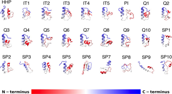
Initial ensemble of the S2 region in the NTD of Esg, obtained by HHpred (HHP), I-Tasser (IT), Phyre2 (PI), QUARK (Q), and SPARK-X (SP) predictors. Each model shows secondary structural elements and is color-coded from red to blue, progressing from the N- to the C-terminus.

The IDPs and IDRs are represented as a dynamic ensemble, which is characterized by different conformations. MD simulations can be used to generate many conformations of the IDP and characterize its conformational ensemble through structural and dynamical information.^3,21 In this work, we have considered running a collection of short (2 μs) simulations using a set of 27 starting models rather than one long simulation, to explore the S2 region conformational ensemble; this strategy has been shown to give more efficient conformational sampling and increases the probability of converging to experimental data.⁴⁸

2.3. Conformational Sampling of the S2 Region

A serious concern with MD simulations is their degree of convergence, and whether the simulation time has been enough to explore the properties of interest. As a first rough measure of the sampling achieved in the 2 μs runs, we calculated the distribution of the C_α-atoms’ root-mean-square deviation (RMSD) to the initial structure of each run to ascertain how much they had wandered from the starting point, and the radius of gyration (R_g), as a measure of compaction.^49,50 An energy landscape built with RMSD and R_g for the 54 μs ensemble (Figure 3A) shows that the conformational distribution is located at two basins, one with low RMSDs and small R_gs, and a larger one with greater variation both in RMSD and R_g. The individual histograms of RMSD and R_g are shown in Figure 3B,C, respectively. The RMSD showed five evident peaks centered near 1.5, 6, 8.5, 9.5, and 13.5 Å, indicating that some runs remained very close to their starting point, while others roamed more freely (Figure 3B); low RMSD happens with low R_g, as expected because more intramolecular contacts hinder conformational exploration. Considering the properties of the amino acid sequences of IDPs, it is possible to estimate their hydrodynamic radii (R_h).⁵¹ For the S2 region with 45 residues, the theoretically estimated R_h value is around 15 Å, and considering that the diameter of a molecule of water is ∼3 Å, the corresponding R_g should be ∼12 Å. The distribution of R_g showed one single peak located between 10 and 11 Å, which corresponds to semicompact conformations (Figure 3C). The results showed that the S2 region ensemble could adopt flexible and heterogeneous conformations, characteristic of an IDP.³ Some force fields and implicit solvent models generate overestimation of compactness for the IDP ensembles,^52,53 and Figure 3 indicates that our simulations also show a modest increase in compaction compared to the predicted R_g. However, chain compaction in IDPs depends on their sequences, for example, the fraction of charged residues and proline content.^54,55 Both R_g and R_h have been related to net charge per residue (NCPR),⁵⁴ where IDPs with NCPR > 0.25 adopt expanded-coil conformations, while NCPR < 0.25 indicates compact globular conformations. The S2 region of Esg has three charged residues, a net charge of +1, 21 hydrophobic, 14 polar, seven aromatic, and six proline residues, and 22 of its 45 amino acids are promoters of disorder. It has an NCPR = 0.022 obtained by the CIDER server,⁵⁶ so it is expected to adopt compact conformations. Figure 3D shows that the average inter-residue distances are larger than those expected for a Lennard-Jones collapsed structure,^53,54 but much smaller than those of a Flory chain of the same length. At this point, it should be stressed that there is no experimental data for S2 that we could use to guide our simulations or as a litmus test of the quality of the data set.

Figure 3.

Structural diversity and degree of compaction of the S2 region of Esg. (A) Energy landscape built with C_α-atom RMSD (Å) and R_g (Å). (B) Histogram of the C_α-atom RMSD (Å) distribution in the ensemble during 54 μs of simulation. (C) Histogram of the R_g (Å) distribution in the ensemble during 54 μs of simulation. (D) Average inter-residue distances (Å) as a function of sequence distance during 54 μs of simulation.

One of the advantages of running multiple independent simulations starting from different structures is that this accelerates convergence in principle. To determine whether 54 μs of simulation is an adequate simulation time, we looked for structurally similar conformations sampled by two different runs. A matrix was generated by the pairwise RMSD between pairs of trajectories, comparing each generated structure in one run to each of the other. Figure 4 shows the heat maps with the pairwise RMSD distance computed between C_α-atoms of the structures generated in the SP8 and SP9 model runs (Figure 4A), and IT4 and SP7 model runs (Figure 4B). Pairs of structures with the smallest pairwise RMSD are in blue, while the largest RMSD is in dark red. The diagonal dark blue line represents the pairwise RMSD comparison of a structure with itself, and the two diagonal squares (frame numbers 1–2000 and 2001–4000) correspond to the comparison within each of the runs; the interesting areas of these plots are the off-diagonal squares, where one run is compared to the other. The pairwise RMSD for each model shows the transition between conformational states within one run.

Figure 4.

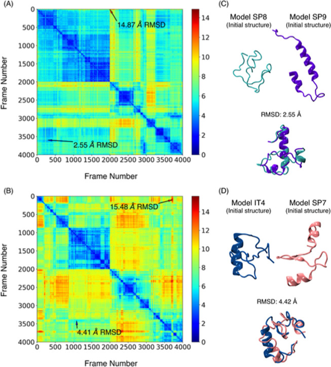
Heat maps representing pairwise RMSD (Å) calculated for the C_α-atoms of the (A) SP8 (frames 1–2000) and SP9 (frames 2001–4000) runs and (B) IT4 (frames 1–2000) and SP7 (frames 2001–4000) runs. Each plot shows the location of the minimum and maximum pairwise RMSD. (C) Initial structures of the SP8 and SP9 models, and overlapping of the minimum of pairwise RMSD. (D) Initial structures of the IT4 and SP7 models, and overlapping of the minimum of pairwise RMSD.

SP8 and SP9 started with a pairwise RMSD of 14.1 Å (Table S3), and during their runs, they generated structures that drifted further apart (maximum pairwise RMSD of 14.87 Å) and also became similar to each other, reaching a pairwise RMSD minimum of 2.55 Å; it can also be seen that low RMSDs occurred multiple times during these two runs (Figure 4A). Similar results were obtained with the IT4 and SP7 trajectories (Figure 4B), where the minimum pairwise RMSD was 4.42 Å and the maximum was 15.48 Å, having started at 10.9 Å. The overlap of the two structures with the minimum pairwise RMSD is shown in Figure 4C,D, illustrating the degree of conformational convergence. This result suggests that simulating each model for 2 μs gives a reasonable run time, so we assume that the structures generated by the 54 μs of MD simulation are a good starting approximation to the diverse conformational space of the S2 region of Esg. A compilation of minimum pairwise RMSDs between all of the models can be found in Table S4; none exceeds 8 Å.

2.4. The S2 Region Harbors an α-MoRF

Inspection of the structures in Figure 2 reveals a prevalence of α-helices. The secondary structure propensity for each amino acid, contained in the structure predictors, yielded two helices: one near the N-terminus in the region from residues 111 to 120 and a second one in the C-terminus, spanning residues 125–150 (Figure 5A). During the simulation, the secondary structure content is lower than that in the initial ensemble; the α-helix conformation of the N-terminus was decreased by ∼30%, while the α-helix conformation of the C-terminus was decreased by ∼10% (Figure 5A). Previous MD simulations have reported that protein unfolding can occur on a picosecond time scale⁴⁹ and it is thus interesting that during 54 μs of simulations, the α-helix conformation remains the most persistent secondary structure in the C-terminus of S2.

Figure 5.

Secondary structure and tertiary contacts of the S2 region. (A) Percentage of the time found as a helix for each residue. (B) Heat map representing the contacts between residue pairs; the dashed line square marks the initial position of helices. (C) Heat map representing the hydrogen bonds involving side chain atoms between residue pairs; the dashed line square marks the C-terminal helix. (D) α-Helix conformation depicting the interactions between E141 with R144 and T145. The main chain is shown as a purple ribbon, and the amino acids are shown as sticks in CPK colors.

Persistent structures require stabilizing interactions. To find those, the total numbers of contacts and hydrogen bonds along the simulations were computed and are presented in the heat maps of Figure 5B,C, respectively. The frequency of interaction between residue pairs is indicated by the color bar, where the dark blue color indicates those contacts with the highest frequency and the yellow color indicates those with the least frequency; white squares away from the diagonal indicate that no interactions were found between that pair of residues. Due to the flexibility of the IDPs, many transient long-range contacts are expected, and these can be seen in the yellow regions. A large probability of contacts between nearby residues in the primary sequence is a hallmark of helical structures,⁵⁷ and these are identified with the black squares of dashed lines in Figure 5B,C.

In Figure 5B,C, the diagonal line represents the interaction of a residue with itself; short-range interactions between residues lie close to the diagonal, and these indicate helices. Off-diagonal interactions are considered long range, and represent tertiary interactions and/or the formation of hairpins. The initial N-terminal α-helices (between residues 111–117 and 124–134) are substantially weakened during the simulations. The region of highest helicity is present in the C-terminal of the S2 region, between the residue regions from 134 to 152, where the most frequent inter-residue contacts and hydrogen bonds occur. Hydrogen bonds contribute to the stability of the protein secondary structure.⁴⁹ The α-helix conformation could be stabilized by interactions between E141 and R144 and T145 residues, which are in the middle of the α-helix (Figure 5D), and are the most frequent side chain hydrogen bond interactions in the ensemble. Together, these results suggest that the S2 region is an IDR and that it could harbor an α-MoRF.

2.5. Mutations to Disrupt the α-MoRF

Oppositely charged residues lead to the formation of salt bridges,^36,58 stabilizing local structures that can be relevant in molecular recognition events.⁵⁷⁻⁶¹ Salt bridges are known to impart local rigidity and the disruption of these interactions increases flexibility,^36,59 which could be associated with “order to disorder” structural transitions in IDPs.³⁶ We have found that the most persistent hydrogen bonds in the ensemble are those between E141, R144, and T145. Interactions between E and R contribute favorably to the stability of helices,^60,61 and interactions between E and R (i + 3, i + 4) are more favorable than the reversed salt bridge.⁶¹ Glutamate can establish side chain–backbone and side chain–side chain interactions,⁶² while threonine has a short polar side chain and has a strong tendency to form hydrogen bonds with neighboring backbone amides, as seen in our simulations. Side chain–backbone hydrogen bonds are determinant to helix formation and the elimination of these interactions destabilizes the helix.⁶² We therefore mutated these residues to eliminate the interactions and disrupt the α-MoRF. E141, R144, and T145 were substituted by residues that cannot form hydrogen bonds and/or have lower helical propensity, such as valine and proline.⁶³ E141 was substituted by leucine (E141L), valine (E141V), and proline (E141P). A double mutant (E141A_T145A) was generated, to eliminate both side chain–side chain and side chain–main chain interactions between E141 and T145. T145 was also substituted by valine (T145V) and R144 by alanine (R144A). Finally, Q149P is an Esg variant in the S2 region that does not show phenotype,⁶⁴ and it was also simulated as a control. We selected four models of the initial ensemble (HHP, PI, SP6, and SP9) and generated the mutants by side chain substitution. Each model was simulated during 6 μs, for a total 24 μs ensemble of each wild-type and mutant S2. Figure 6 shows the secondary structure of the α-MoRF region (from residues 134 to 152) of each mutant compared to that in the wild-type. The mutants showed either modest changes or local increases of helicity with respect to the wild-type, toward the N-terminus or the C-terminus of the helix. The Q149P and the double mutant disrupted the C-terminus of the α-MoRF; the loss of structure for Q149P might indicate that the α-MoRF need not extend that far to be functional. The breaking of intramolecular hydrogen bonds has previously been identified as a key step in protein unfolding,⁴⁹ but the hydrogen bonds involving side chain atoms in the mutants did not show significant differences compared to the wild-type, and their frequency was very low. On the other hand, the numbers of carbon–carbon contacts increased, especially between the α-MoRF region and the rest of S2; these contacts were not present significantly in the wild-type variant (Table S5).

Figure 6.

Percentage of the helicity per residue of the α-MoRF (from residues 134 to 152) of each mutant, with respect to the wild-type (black line). The value for each residue is marked by a dot.

The mutants have interactions in common, involving aromatic residues on both the helix (Y138, F142, and Y143, surrounding the mutated residues) and outside of it (Y125, Y128, W130, and F133), which stabilize the helical structure (Figure S1 and Table S5) by the possible formation of a small hydrophobic core. The S2 region is enriched in aromatic residues and prolines that could be involved also in the stabilization of the α-MoRF. Recently, it was reported that interactions between prolines and aromatic residues in positions i ± 1 and i – 2 can form incipient structural nucleation sites in IDPs.⁶⁵ The frequency of these interactions in the simulations is compiled in Table S6 and representative structures depicting these are included in Figure S2. These interactions are common in the simulations and are notably enriched for the E141A_T145A double mutant in all proline–aromatic pairs, and approximately one helix turn away from the mutation site in the E141P variant. All of the proline residues in the simulations are in the trans configuration. To explore biases in their conformational sampling, we calculated the Ramachandran plot for the wild-type 54 μs ensemble (Figure S3), which shows populations of both the polyproline-II and α helix basins, with a small preference for the latter.

2.6. Validation of the Force Field and Solvent Model Used in the Simulations

A well-known issue in the simulation of IDPs is the artificial increase in both secondary and tertiary structures. A modified version of CHARMM36 (CHARMM36m) corrects the excessive population of the left-handed α-helix (α_L-helix) conformation generated in simulations with CHARMM36.⁴² This new release was not available when this project started, so all of the runs were carried out with the same force field for consistency. To determine the level of inaccuracy of our description of S2, we calculated the α_L-helix population of the 54 μs of the S2 region ensemble, obtaining a 1.36% population, which is significantly lower than that found in other simulations generated with CHARMM36 of IDPs (between 5.7 and 20%), and considered it within the margin of error of the experimental value.^42,66

One of the standard peptides used for the validation of force fields is (AAQAA)₃, a helical peptide that has been well studied and characterized experimentally to understand the helix–coil transitions.^39,42,66 (AAQAA)₃ has ∼19–21% helical content.^42,66 We carried out two 16 μs of simulations of (AAQAA)₃ using exactly the same protocol as that for the S2 runs. This particular combination of CHARMM36 with the GBSA solvent (as implemented in NAMD) has not been benchmarked with (AAQAA)₃, despite having been used to simulate other IDPs, as shown in Tables S1 and S2. One of the simulations started from a perfect helix (100% helicity) and the other from a completely extended conformation (0% helicity), therefore accounting for the 50% helicity per residue for the starting structures. Figure 7 shows that (AAQAA)₃ exchanges frequently between coil and helical conformations (Figure 7A,C), and its average helical content during the 32 μs ensemble was ∼24%, indicating that CHARMM36 with GBSA provides a reasonable balance between helix and coil conformations for (AAQAA)₃. Close inspection of Figure 7A shows that the two 16 μs runs had a different behavior: one with an excess of helix and the other with long periods of absence of helices. This indicates that even for simple systems like this small peptide, having seen multiple helix–coil transitions does not guarantee sufficient sampling, so at least two runs starting from different structures should be made of the same system.

Figure 7.

Ensemble of (AAQAA)₃ during 32 μs of MD simulation. (A) Fraction helix of (AAQAA)₃ computed over 10 ns blocks; the first 16 μs correspond to the simulation starting from the extended conformation and the last 16 μs correspond to the simulation starting from a perfect helix. (B) Percentage of the helicity per residue, averaged over the 32 μs (red line) compared to the initial ensemble (blue line). (C) (AAQAA)₃ conformations representing coil–helix transitions at different times during the simulations.

Regarding the stabilization of the S2 mutants described above, there remains an unexplored issue for which we have no adequate control or experimental information for contrast. Given that the helices appear to be stabilized by aromatic interactions, this could be due to a real nucleating event caused by increasing locally the hydrophobicity of the helix, as all of the mutations changed a charged or polar residue for a hydrophobic one. Alternatively, this could reflect an imbalance in the polar and nonpolar surface descriptions in the GBSA model. To explore the possibility of indiscriminate hydrophobic collapse, we calculated the contact map for the 32 μs simulation of (AAQAA)₃, shown in Figure S4; the structures depicting the most common interactions are included in Figure S5, and, as expected because of their greater number of carbon atoms, involve the glutamine residues. It is clear from this contact map that no long-range contacts are promoted in this peptide, which is 80% hydrophobic. Therefore, we are currently inclined to ascribe the stabilization of the S2 mutants to bona fide interactions, as the simulations of the wild-type and mutant S2 started from the same four conformations and were run with the same protocol, for three times as long as the time we determined was enough to see similar conformations sampled by different runs (see Figure 4).

3. Conclusions

In this work, we investigated the presence of MoRFs in the NTD of the transcription factor Esg by MD simulations using the CHARMM36 force field and GBSA as an implicit solvent model. In summary, we have detected a region with a high probability to be ordered that we have called the S2 region (from residues 111 to 155). The conformational ensemble of this region contains residual structure as an α-MoRF that persists during 54 μs of MD simulation. In addition, point mutations were built to disrupt this putative α-MoRF and probe its stability during 24 μs of simulation. However, some of the mutants showed an increase of helicity at the α-MoRF, as a consequence of an increase in long-distance contacts with residues outside the MoRF. To validate our simulation protocol, we have evaluated the propensity of the α_L-helix in the 54 μs of MD simulation, and we found that it is significantly lower than that found in ensembles generated with CHARMM36 for other IDPs and in agreement with experimental data. Also, we carried out 32 μs of simulation of (AAQAA)₃ and its average helical content was ∼24%, a value close to the ∼20% measured experimentally, indicating that CHARMM36 together with GBSA provides a good balance between helix and coil conformations for this system. The lack of long-range contacts in these simulations suggests that there is a reasonable balance in the description of polar and nonpolar interactions in this particular combination of a protein force field and an implicit solvent model. Therefore, the stabilization of the MoRF that we found with the mutants could be due to the increase in hydrophobicity at the surface of the helix, which nucleates the interaction with a group of aromatic residues within and outside the MoRF. Assuming that the interactions are correctly described, as we see no such clustering in the wild-type S2 or in the control peptide, we can now propose a set of mutations that should eliminate the MoRF: E141P as a helix breaker, and W130A and F142A as disruptors of the most common long-range interaction. These can be tested in in vitro assays as peptides, or in the context of the full protein in in vivo studies, contributing to the functional annotation of a poorly characterized domain in an important transcription factor, conserved in all multicellular animals.

4. Methods

4.1. Disorder Analysis

The sequence of the full Esg protein (470 amino acids) was obtained from Uniprot,⁶⁷ (Uniprot ID: P25932, htttp://www.uniprot.org/). Disorder analysis was performed using the disorder predictors: MetaDisorder,⁶⁸ MFDp2,⁶⁹ AUCPred,⁷⁰ and SPOT-disorder,⁷¹ which yield the best results as recently reviewed.⁷² Metadisorder is a metaserver that utilizes different disorder predictors and calculates an average of the output of those results, thus improving the prediction accuracy. The output of the three variants of Metadisorder was used: MetaDisorderMD, MetaDisorderMD2 (a variant of MetaDisorderMD with a different scoring function), and MetaDisorderMD3 (based on fold recognition methods). MFDp2 (http://biomine.cs.vcu.edu/servers/MFDp2/) predicts the disorder at the sequence and residue levels. AUCPred and SPOT-disorder can predict short and long IDRs. AUCpreD (http://raptorx.uchicago.edu/StructurePropertyPred/predict/) predicts disorder considering information from the sequence, evolution, and structural levels, while SPOT-disorder (https://sparks-lab.org/server/spot-disorder-single/) considers sequence-level information. These predictors assign a disorder score to each amino acid of the query sequence. The disorder probability of the Esg protein was calculated by averaging the results obtained by all of the predictors. Residues with scores >0.5 were considered to be disordered. The result was plotted using Matplotlib 2.2.3.⁷³

4.2. Generation of Starting Structures for the Simulations

To obtain initial structures of the S2 region (residues 111–155: ¹¹¹AAAAAASVVVPTPTYPKYPWNNFHMSPYTAEFYRTINQQGHQILP¹⁵⁵) of Esg, the predictors HHPred⁷⁴ (https://toolkit.tuebingen.mpg.de/tools/hhpred), I-Tasser⁷⁵ (https://zhanglab.ccmb.med.umich.edu/I-TASSER/), Phyre2⁷⁶ (http://www.sbg.bio.ic.ac.uk/;phyre2/html/page.cgi?id=index), QUARK⁷⁷ (https://zhanglab.ccmb.med.umich.edu/QUARK/), and SPARKS-X⁷⁸ (https://sparks-lab.org/server/sparks-x/) were used. These predictors use homology modeling, fold recognition, and ab initio methods. Through this, 27 structural models were obtained as an initial ensemble, which were visualized using VMD 1.9.2;⁷⁹ the structures were prepared with CHARMM-GUI⁸⁰ for their simulation. The N- and C-termini were charged, histidine was neutral (protonated in the δ nitrogen), and glutamate and lysine were charged.

4.3. Generation of the Mutant Models

To generate the mutant models, four models of the initial ensemble that presented structural diversity were selected. The selected models had a radius of gyration (R_g) between 10 and 11 Å, and had either wandered substantially (PI) or not (HHP) from their initial structure during the 2 μs simulations of the wild-type S2. We also chose the model with the longest continuous α-helix (SP9), as well as the model with a β-sheet (SP6). The mutants E141P, E141L, E141V, E141A_T145A, R144A, T145V, and Q149P were built using CHARMM-GUI⁸⁰ in the context of the four models. The N- and C-termini were charged, histidine was neutral (protonated in the δ nitrogen), and glutamate and lysine were charged.

4.4. Molecular Dynamics Simulations

For each model, the inputs were generated using CHARMM-GUI.⁸⁰ All of the MD simulations were performed with the software NAMD 2.10⁸¹ (http://www.ks.uiuc.edu/Research/namd/), using the CHARMM36 force field⁸² (http://mackerell.umaryland.edu/charmm_ff.shtml), the generalized Born/surface area (GBSA) model of implicit solvent⁸³ with the default parameters suggested by NAMD, and 2 fs time steps. All simulations were carried out at a constant temperature (298 K) with a Langevin thermostat. An ε-value of 80, viscosity of 91 cps, and ionic strength of 0.15 M were used to simulate an aqueous solution environment. The SHAKE method was used to keep all bonds involving hydrogen atoms rigid. The list of neighbors was calculated with a 14 Å cutoff every 10 steps, and the noncovalent interactions had a 12 Å cutoff, with switching at 10 Å. Each model was submitted to 2000 steps of structural minimization in vacuum to eliminate clashes before the MD runs. The MD simulations were carried out for 2 μs for each model of the S2 region, and the trajectories were stored every 1 ps, yielding the 54 μs MD ensemble.

4.5. Molecular Dynamics Simulation of the Mutants

These were carried under the same conditions, except that each model was simulated during 6 μs, yielding a 24 μs ensemble for each variant. The simulations of the wild-type models were extended to 6 μs each.

4.6. α_L Sampling Characterization

The dihedral angles Φ and φ of the 54 μs MD ensemble were calculated with CHARMM38. The selected dihedral angles Φ and φ were those with at least three consecutive residues with values in the α_L region (30° < Φ < 100° and 7° < φ < 67°).⁴² The probability of α_L is calculated as the fraction of the ensemble that contains α_L helices.

4.7. Molecular Dynamics Simulation of (AAQAA)₃

A helical and extended model of (AAQAA)₃ was built using the Chimera software.⁸⁴ N- and C-termini were capped by acetylation and amidation, respectively, using CHARMM-GUI.⁸⁰ Each model was simulated under the same conditions as the models of the S2 region of Esg, during 16 μs.

4.8. Trajectory Analysis

The analysis of the trajectories was performed using CARMA⁸⁵ to calculate the secondary structure. CHARMM38 was used to calculate the root-mean-square deviation (RMSD) with respect to the starting structures, radius of gyration (R_g), main chain dihedral angles, contacts (carbon–carbon distances within 6 Å), and hydrogen bonds (2.4 Å distance between hydrogen and heavy atom, no angle restriction). Contacts and hydrogen bonds were calculated for atom pairs and then all pairs belonging to each particular residue–residue pair were added; therefore, frequencies above 100% represent more than one consistent contact or hydrogen bond present during the whole simulation ensemble. The results were plotted with Matplotlib 2.2.3.⁷³

Glossary

Abbreviations

MoRF

molecular recognition feature

IDP

intrinsically disordered protein

IDR

Intrinsically disordered region

Esg

Escargot

MD

molecular dynamics

MC

Monte Carlo

GBSA

generalized Born and surface area continuum solvation

ZNF

zinc finger

NTD

N-terminal domain

RMSD

root-mean-square deviation

R_g

radius of gyration

Supporting Information Available

The Supporting Information is available free of charge at https://pubs.acs.org/doi/10.1021/acsomega.0c02051.

• Summary of IDP simulations of the past 5 years; summary of (AAQAA)₃ simulations; pairwise initial RMSDs; minimum pairwise RMSD between runs after 2 μs of simulation; most frequent long-distance contacts stabilizing the MoRF; and most frequent interactions between aromatic residues and prolines in the MoRF (Tables S1–S6). Contact map of the residues in the MoRF and snapshot showing one of the stabilizing long-distance contacts, for mutant E141V; snapshots of the most frequent interactions between aromatic and proline residues in the S2 region for mutant E14A_T145A; Ramachandran plot for proline residues in wild-type S2; contact map for (AAQAA)₃; and snapshots of the most frequent interactions in (AAQAA)₃ (Figures S1–S5) (PDF)

The authors declare no competing financial interest.

Author Status

^§ On sabbatical leave at Departamento de Medicina Molecular y Bioprocesos, Instituto de Biotecnología, Universidad Nacional Autónoma de México, Av. Universidad 2001, Col. Chamilpa, 62210 Cuernavaca, Morelos, México.

References

- Ouyang Y.; Zhao L.; Zhang Z. Characterization of the structural ensembles of p53 TAD2 by molecular dynamics simulations with different force fields. Phys. Chem. Chem. Phys. 2018, 20, 8676–8684. 10.1039/C8CP00067K. [DOI] [PubMed] [Google Scholar]
- Shabane P. S.; Izadi S.; Onufriev A. V. General Purpose Water Model Can Improve Atomistic Simulations of Intrinsically Disordered Proteins. J. Chem. Theory Comput. 2019, 15, 2620–2634. 10.1021/acs.jctc.8b01123. [DOI] [PubMed] [Google Scholar]
- Shrestha U. R.; Juneja P.; Zhang Q.; Gurumoorthy V.; Borreguero J. M.; Urban V.; Cheng X.; Pingali S. V.; Smith J. C.; O’Neill H. M.; Petridis L. Generation of the configurational ensemble of an intrinsically disordered protein from unbiased molecular dynamics simulation. Proc. Natl. Acad. Sci. U.S.A. 2019, 116, 20446–20452. 10.1073/pnas.1907251116. [DOI] [PMC free article] [PubMed] [Google Scholar]
- Keppel T. R.; Weis D. D. Mapping residual structure in intrinsically disordered proteins at residue resolution using millisecond hydrogen/deuterium exchange and residue averaging. J. Am. Soc. Mass Spectrom. 2015, 26, 547–554. 10.1007/s13361-014-1033-6. [DOI] [PubMed] [Google Scholar]
- Gianni S.; Dogan J.; Jemth P. Distinguishing induced fit from conformational selection. Biophys. Chem. 2014, 189, 33–39. 10.1016/j.bpc.2014.03.003. [DOI] [PubMed] [Google Scholar]
- Toto A.; Malagrinò F.; Visconti L.; Troilo F.; Pagano L.; Brunori M.; Jemth P.; Gianni S. Templated folding of intrinsically disordered proteins. J. Biol. Chem. 2020, 295, 6586–6593. 10.1074/jbc.REV120.012413. [DOI] [PMC free article] [PubMed] [Google Scholar]
- Zhang W.; Ganguly D.; Chen J. Residual structures, conformational fluctuations, and electrostatic interactions in the synergistic folding of two intrinsically disordered proteins. PLoS Comput. Biol. 2012, 8, e1002353 10.1371/journal.pcbi.1002353. [DOI] [PMC free article] [PubMed] [Google Scholar]
- Click T. H.; Ganguly D.; Chen J. Intrinsically disordered proteins in a physics-based world. Int. J. Mol. Sci. 2010, 11, 5292–5309. 10.3390/ijms11125292. [DOI] [PMC free article] [PubMed] [Google Scholar]
- Pinheiro A. S.; Marsh J. A.; Forman-Kay J. D.; Peti W. Structural signature of the MYPT1-PP1 interaction. J. Am. Chem. Soc. 2011, 133, 73–80. 10.1021/ja107810r. [DOI] [PMC free article] [PubMed] [Google Scholar]
- Fuxreiter M.; Simon I.; Friedrich P.; Tompa P. Preformed structural elements feature in partner recognition by intrinsically unstructured proteins. J. Mol. Biol. 2004, 338, 1015–1026. 10.1016/j.jmb.2004.03.017. [DOI] [PubMed] [Google Scholar]
- Uversky V. N.Intrinsic Disorder, Protein–Protein Interactions, and Disease. Advances in Protein Chemistry and Structural Biology; Academic Press Inc, 2018; pp 85–121. [DOI] [PubMed] [Google Scholar]
- Frege T.; Uversky V. N. Intrinsically disordered proteins in the nucleus of human cells. Biochem. Biophys. Rep. 2015, 1, 33–51. 10.1016/j.bbrep.2015.03.003. [DOI] [PMC free article] [PubMed] [Google Scholar]
- Habchi J.; Tompa P.; Longhi S.; Uversky V. N. Introducing protein intrinsic disorder. Chem. Rev. 2014, 114, 6561–6588. 10.1021/cr400514h. [DOI] [PubMed] [Google Scholar]
- Uversky V. N. Dancing protein clouds: The strange biology and chaotic physics of intrinsically disordered proteins. J. Biol. Chem. 2016, 291, 6681–6688. 10.1074/jbc.R115.685859. [DOI] [PMC free article] [PubMed] [Google Scholar]
- Tompa P.; Fersht A.. Extension of the Structure–Function Paradigm. Structure and Function of Intrinsically Disordered Proteins; CRC Press, 2009; pp 205–236. [Google Scholar]
- Staby L.; O’Shea C.; Willemoës M.; Theisen F.; Kragelund B. B.; Skriver K. Eukaryotic transcription factors: Paradigms of protein intrinsic disorder. Biochem. J. 2017, 474, 2509–2532. 10.1042/BCJ20160631. [DOI] [PubMed] [Google Scholar]
- Liu J.; Perumal N. B.; Oldfield C. J.; Su E. W.; Uversky V. N.; Dunker A. K. Intrinsic disorder in transcription factors. Biochemistry 2006, 45, 6873–6888. 10.1021/bi0602718. [DOI] [PMC free article] [PubMed] [Google Scholar]
- Kukharenko O.; Sawade K.; Steuer J.; Peter C. Using Dimensionality Reduction to Systematically Expand Conformational Sampling of Intrinsically Disordered Peptides. J. Chem. Theory Comput. 2016, 12, 4726–4734. 10.1021/acs.jctc.6b00503. [DOI] [PubMed] [Google Scholar]
- Best R. B. Emerging consensus on the collapse of unfolded and intrinsically disordered proteins in water. Curr. Opin. Struct. Biol. 2020, 60, 27–38. 10.1016/j.sbi.2019.10.009. [DOI] [PMC free article] [PubMed] [Google Scholar]
- Chong S.-H.; Chatterjee P.; Ham S. Computer Simulations of Intrinsically Disordered Proteins. Annu. Rev. Phys. Chem. 2017, 68, 117–134. 10.1146/annurev-physchem-052516-050843. [DOI] [PubMed] [Google Scholar]
- Das P.; Matysiak S.; Mittal J. Looking at the Disordered Proteins through the Computational Microscope. ACS Cent. Sci. 2018, 4, 534–542. 10.1021/acscentsci.7b00626. [DOI] [PMC free article] [PubMed] [Google Scholar]
- Bottaro S.; Lindorff-Larsen K.; Best R. B. Variational optimization of an all-atom implicit solvent force field to match explicit solvent simulation data. J. Chem. Theory Comput. 2013, 9, 5641–5652. 10.1021/ct400730n. [DOI] [PMC free article] [PubMed] [Google Scholar]
- Juneja A.; Ito M.; Nilsson L. Implicit solvent models and stabilizing effects of mutations and ligands on the unfolding of the amyloid β-peptide central helix. J. Chem. Theory Comput. 2013, 9, 834–846. 10.1021/ct300941v. [DOI] [PubMed] [Google Scholar]
- Onufriev A.Implicit Solvent Models in Molecular Dynamics Simulations: A Brief Overview. Annual Reports in Computational Chemistry; Elsevier BV, 2008; pp 125–137. [Google Scholar]
- Ganguly D.; Chen J. Atomistic details of the disordered states of KID and pKID. implications in coupled binding and folding. J. Am. Chem. Soc. 2009, 131, 5214–5223. 10.1021/ja808999m. [DOI] [PubMed] [Google Scholar]
- Umezawa K.; Ikebe J.; Takano M.; Nakamura H.; Higo J. Conformational ensembles of an intrinsically disordered protein pKID with and without a KIX domain in explicit solvent investigated by all-atom multicanonical molecular dynamics. Biomolecules 2012, 2, 104–121. 10.3390/biom2010104. [DOI] [PMC free article] [PubMed] [Google Scholar]
- Sridhar A.; Orozco M.; Collepardo-Guevara R. Protein disorder-to-order transition enhances the nucleosome-binding affinity of H1. Nucleic Acids Res. 2020, 48, 5318–5331. 10.1093/nar/gkaa285. [DOI] [PMC free article] [PubMed] [Google Scholar]
- Scholes N. S.; Weinzierl R. O. J. Molecular Dynamics of ‘Fuzzy’ Transcriptional Activator-Coactivator Interactions. PLoS Comput. Biol. 2016, 12, e1004935 10.1371/journal.pcbi.1004935. [DOI] [PMC free article] [PubMed] [Google Scholar]
- Wang J.; Cao Z.; Li S. Molecular Dynamics Simulations of Intrinsically Disordered Proteins in Human Diseases. Curr. Comput. Aided-Drug Des. 2009, 5, 280–287. 10.2174/157340909789577865. [DOI] [Google Scholar]
- Anandakrishnan R.; Drozdetski A.; Walker R. C.; Onufriev A. V. Speed of conformational change: Comparing explicit and implicit solvent molecular dynamics simulations. Biophys. J. 2015, 108, 1153–1164. 10.1016/j.bpj.2014.12.047. [DOI] [PMC free article] [PubMed] [Google Scholar]
- Vitalis A.; Pappu R. V. ABSINTH: A new continuum solvation model for simulations of polypeptides in aqueous solutions. J. Comput. Chem. 2009, 30, 673–699. 10.1002/jcc.21005. [DOI] [PMC free article] [PubMed] [Google Scholar]
- Wu K. P.; Weinstock D. S.; Narayanan C.; Levy R. M.; Baum J. Structural Reorganization of α-Synuclein at Low pH Observed by NMR and REMD Simulations. J. Mol. Biol. 2009, 391, 784–796. 10.1016/j.jmb.2009.06.063. [DOI] [PMC free article] [PubMed] [Google Scholar]
- Mao A. H.; Crick S. L.; Vitalis A.; Chicoine C. L.; Pappu R. V. Net charge per residue modulates conformational ensembles of intrinsically disordered proteins. Proc. Natl. Acad. Sci. U.S.A. 2010, 107, 8183–8188. 10.1073/pnas.0911107107. [DOI] [PMC free article] [PubMed] [Google Scholar]
- Piana S.; Donchev A. G.; Robustelli P.; Shaw D. E. Water dispersion interactions strongly influence simulated structural properties of disordered protein states. J. Phys. Chem. B 2015, 119, 5113–5123. 10.1021/jp508971m. [DOI] [PubMed] [Google Scholar]
- Henriques J.; Cragnell C.; Skepö M. Molecular Dynamics Simulations of Intrinsically Disordered Proteins: Force Field Evaluation and Comparison with Experiment. J. Chem. Theory Comput. 2015, 11, 3420–3431. 10.1021/ct501178z. [DOI] [PubMed] [Google Scholar]
- Basu S.; Biswas P. Salt-bridge dynamics in intrinsically disordered proteins: A trade-off between electrostatic interactions and structural flexibility. Biochim. Biophys. Acta, Proteins Proteomics 2018, 1866, 624–641. 10.1016/j.bbapap.2018.03.002. [DOI] [PubMed] [Google Scholar]
- Voelz V. A.; Singh V. R.; Wedemeyer W. J.; Lapidus L. J.; Pande V. S. Unfolded-state dynamics and structure of protein L characterized by simulation and experiment. J. Am. Chem. Soc. 2010, 132, 4702–4709. 10.1021/ja908369h. [DOI] [PMC free article] [PubMed] [Google Scholar]
- Rhee Y. M.; Sorin E. J.; Jayachandran G.; Lindahl E.; Pande V. S. Simulations of the role of water in the protein-folding mechanism. Proc. Natl. Acad. Sci. U.S.A. 2004, 101, 6456–6461. 10.1073/pnas.0307898101. [DOI] [PMC free article] [PubMed] [Google Scholar]
- Lee K. H.; Chen J. Optimization of the GBMV2 implicit solvent force field for accurate simulation of protein conformational equilibria. J. Comput. Chem. 2017, 38, 1332–1341. 10.1002/jcc.24734. [DOI] [PMC free article] [PubMed] [Google Scholar]
- Robustelli P.; Piana S.; Shaw D. E. Developing a molecular dynamics force field for both folded and disordered protein states. Proc. Natl. Acad. Sci. U.S.A. 2018, 115, E4758–E4766. 10.1073/pnas.1800690115. [DOI] [PMC free article] [PubMed] [Google Scholar]
- Beauchamp K. A.; Lin Y. S.; Das R.; Pande V. S. Are protein force fields getting better? A systematic benchmark on 524 diverse NMR measurements. J. Chem. Theory Comput. 2012, 8, 1409–1414. 10.1021/ct2007814. [DOI] [PMC free article] [PubMed] [Google Scholar]
- Huang J.; Rauscher S.; Nawrocki G.; Ran T.; Feig M.; De Groot B. L.; Grubmüller H.; MacKerell A. D. CHARMM36m: An improved force field for folded and intrinsically disordered proteins. Nat. Methods 2017, 14, 71–73. 10.1038/nmeth.4067. [DOI] [PMC free article] [PubMed] [Google Scholar]
- Liu H.; Song D.; Zhang Y.; Yang S.; Luo R.; Chen H. F. Extensive tests and evaluation of the CHARMM36IDPSFF force field for intrinsically disordered proteins and folded proteins. Phys. Chem. Chem. Phys. 2019, 21, 21918–21931. 10.1039/C9CP03434J. [DOI] [PMC free article] [PubMed] [Google Scholar]
- Yang D. J.; Chung J. Y.; Lee S. J.; Park S. Y.; Pyo J. H.; Ha N. C.; Yoo M. A.; Park B. J. Slug, mammalian homologue gene of Drosophila escargot, promotes neuronal-differentiation through suppression of HEB/daughtherless. Cell Cycle 2010, 9, 2861–2874. 10.4161/cc.9.14.12247. [DOI] [PubMed] [Google Scholar]
- Hemavathy K.; Guru S. C.; Harris J.; Chen J. D.; Ip Y. T. Human Slug Is a Repressor That Localizes to Sites of Active Transcription. Mol. Cell. Biol. 2000, 20, 5087–5095. 10.1128/MCB.20.14.5087-5095.2000. [DOI] [PMC free article] [PubMed] [Google Scholar]
- Villarejo A.; Cortés-Cabrera Á.; Molina-Ortíz P.; Portillo F.; Cano A. Differential role of snail1 and snail2 zinc fingers in E-cadherin repression and epithelial to mesenchymal transition. J. Biol. Chem. 2014, 289, 930–941. 10.1074/jbc.M113.528026. [DOI] [PMC free article] [PubMed] [Google Scholar]
- Voog J.; Sandall S. L.; Hime G. R.; Resende L. P. F.; Loza-Coll M.; Aslanian A.; Yates J. R.; Hunter T.; Fuller M. T.; Jones D. L. Escargot Restricts Niche Cell to Stem Cell Conversion in the Drosophila Testis. Cell Rep. 2014, 7, 722–734. 10.1016/j.celrep.2014.04.025. [DOI] [PMC free article] [PubMed] [Google Scholar]
- Sethi A.; Tian J.; Vu D. M.; Gnanakaran S. Identification of minimally interacting modules in an intrinsically disordered protein. Biophys. J. 2012, 103, 748–757. 10.1016/j.bpj.2012.06.052. [DOI] [PMC free article] [PubMed] [Google Scholar]
- Navarro-Retamal C.; Bremer A.; Alzate-Morales J.; Caballero J.; Hincha D. K.; González W.; Thalhammer A. Molecular dynamics simulations and CD spectroscopy reveal hydration-induced unfolding of the intrinsically disordered LEA proteins COR15A and COR15B from: Arabidopsis thaliana. Phys. Chem. Chem. Phys. 2016, 18, 25806–25816. 10.1039/C6CP02272C. [DOI] [PubMed] [Google Scholar]
- Ilizaliturri-Flores I.; Correa-Basurto J.; Bello M.; Rosas-Trigueros J. L.; Zamora-López B.; Benítez-Cardoza C. G.; Zamorano-Carrillo A. Mapping the intrinsically disordered properties of the flexible loop domain of Bcl-2: a molecular dynamics simulation study. J. Mol. Model. 2016, 22, 98 10.1007/s00894-016-2940-1. [DOI] [PubMed] [Google Scholar]
- Tomasso M. E.; Tarver M. J.; Devarajan D.; Whitten S. T. Hydrodynamic Radii of Intrinsically Disordered Proteins Determined from Experimental Polyproline II Propensities. PLoS Comput. Biol. 2016, 12, e1004686 10.1371/journal.pcbi.1004686. [DOI] [PMC free article] [PubMed] [Google Scholar]
- Guo X.; Han J.; Luo R.; Chen H. F. Conformation dynamics of the intrinsically disordered protein c-Myb with the ff99IDPs force field. RSC Adv. 2017, 7, 29713–29721. 10.1039/C7RA04133K. [DOI] [PMC free article] [PubMed] [Google Scholar]
- Song D.; Luo R.; Chen H. F. The IDP-Specific Force Field ff14IDPSFF Improves the Conformer Sampling of Intrinsically Disordered Proteins. J. Chem. Inf. Model. 2017, 57, 1166–1178. 10.1021/acs.jcim.7b00135. [DOI] [PMC free article] [PubMed] [Google Scholar]
- Sherry K. P.; Das R. K.; Pappu R. V.; Barrick D. Control of transcriptional activity by design of charge patterning in the intrinsically disordered RAM region of the Notch receptor. Proc. Natl. Acad. Sci. U.S.A. 2017, 114, E9243–E9252. 10.1073/pnas.1706083114. [DOI] [PMC free article] [PubMed] [Google Scholar]
- Das R. K.; Pappu R. V. Conformations of intrinsically disordered proteins are influenced by linear sequence distributions of oppositely charged residues. Proc. Natl. Acad. Sci. U.S.A. 2013, 110, 13392–13397. 10.1073/pnas.1304749110. [DOI] [PMC free article] [PubMed] [Google Scholar]
- Holehouse A. S.; Das R. K.; Ahad J. N.; Richardson M. O. G.; Pappu R. V. CIDER: Resources to Analyze Sequence-Ensemble Relationships of Intrinsically Disordered Proteins. Biophys. J. 2017, 112, 16–21. 10.1016/j.bpj.2016.11.3200. [DOI] [PMC free article] [PubMed] [Google Scholar]
- Carballo-Pacheco M.; Strodel B. Comparison of force fields for Alzheimer’s A β42: A case study for intrinsically disordered proteins. Protein Sci. 2017, 26, 174–185. 10.1002/pro.3064. [DOI] [PMC free article] [PubMed] [Google Scholar]
- Donald J. E.; Kulp D. W.; DeGrado W. F. Salt bridges: Geometrically specific, designable interactions. Proteins: Struct., Funct., Bioinf. 2011, 79, 898–915. 10.1002/prot.22927. [DOI] [PMC free article] [PubMed] [Google Scholar]
- Zhang X.; Li L.; Li N.; Shu X.; Zhou L.; Lü S.; Chen S.; Mao D.; Long M. Salt bridge interactions within the β2 integrin α7 helix mediate force-induced binding and shear resistance ability. FEBS J. 2018, 285, 261–274. 10.1111/febs.14335. [DOI] [PubMed] [Google Scholar]
- Basu S.; Mukharjee D. Salt-bridge networks within globular and disordered proteins: characterizing trends for designable interactions. J. Mol. Model. 2017, 23, 206 10.1007/s00894-017-3376-y. [DOI] [PubMed] [Google Scholar]
- Huerta-Viga A.; Amirjalayer S.; Domingos S. R.; Meuzelaar H.; Rupenyan A.; Woutersen S. The structure of salt bridges between Arg+ and Glu- in peptides investigated with 2D-IR spectroscopy: Evidence for two distinct hydrogen-bond geometries. J. Chem. Phys. 2015, 142, 212444 10.1063/1.4921064. [DOI] [PubMed] [Google Scholar]
- Vijayakumar M.; Qian H.; Zhou H. X. Hydrogen bonds between short polar side chains and peptide backbone: Prevalence in proteins and effects on helix-forming propensities. Proteins: Struct., Funct., Genet. 1999, 34, 497–507. . [DOI] [PubMed] [Google Scholar]
- Wang J.; Feng J. A. Exploring the sequence patterns in the α-helices of proteins. Protein Eng. 2003, 16, 799–807. 10.1093/protein/gzg101. [DOI] [PubMed] [Google Scholar]
- Fuse N.; Hirose S.; Hayashi S. Diploidy of Drosophila imaginal cells is maintained by a transcriptional repressor encoded by escargot. Genes Dev. 1994, 8, 2270–2281. 10.1101/gad.8.19.2270. [DOI] [PubMed] [Google Scholar]
- Mateos B.; Conrad-Billroth C.; Schiavina M.; Beier A.; Kontaxis G.; Konrat R.; Felli I. C.; Pierattelli R. The Ambivalent Role of Proline Residues in an Intrinsically Disordered Protein: From Disorder Promoters to Compaction Facilitators. J. Mol. Biol. 2019, 432, 3093–3111. 10.1016/j.jmb.2019.11.015. [DOI] [PubMed] [Google Scholar]
- Huang J.; Mackerell A. D. Induction of peptide bond dipoles drives cooperative helix formation in the (AAQAA)3 peptide. Biophys. J. 2014, 107, 991–997. 10.1016/j.bpj.2014.06.038. [DOI] [PMC free article] [PubMed] [Google Scholar]
- Bateman A. UniProt: A worldwide hub of protein knowledge. Nucleic Acids Res. 2019, 47, D506–D515. 10.1093/nar/gky1049. [DOI] [PMC free article] [PubMed] [Google Scholar]
- Kozlowski L. P.; Bujnicki J. M. MetaDisorder: a meta-server for the prediction of intrinsic disorder in proteins. BMC Bioinformatics 2012, 13, 111 10.1186/1471-2105-13-111. [DOI] [PMC free article] [PubMed] [Google Scholar]
- Mizianty M. J.; Peng Z.; Kurgan L. MFDp2: Accurate predictor of disorder in proteins by fusion of disorder probabilities, content and profiles. Intrinsically Disord. Proteins 2013, 1, e24428 10.4161/idp.24428. [DOI] [PMC free article] [PubMed] [Google Scholar]
- Wang S.; Ma J.; Xu J. AUCpreD: Proteome-level protein disorder prediction by AUC-maximized deep convolutional neural fields. Bioinformatics 2016, i672–i679. 10.1093/bioinformatics/btw446. [DOI] [PMC free article] [PubMed] [Google Scholar]
- Hanson J.; Yang Y.; Paliwal K.; Zhou Y. Improving protein disorder prediction by deep bidirectional long short-term memory recurrent neural networks. Bioinformatics 2017, 33, 685–692. 10.1093/bioinformatics/btw678. [DOI] [PubMed] [Google Scholar]
- Nielsen J. T.; Mulder F. A. A. Quality and bias of protein disorder predictors. Sci. Rep. 2019, 9, 5137 10.1038/s41598-019-41644-w. [DOI] [PMC free article] [PubMed] [Google Scholar]
- Caswell T. A.; Droettboom M.; Hunter J.; Firing E.; Lee A.; Nielsen J. H.; Andrade E. S.; de Stansby D.; Varoquaux N.; Klymak J.; Root B.; Elson P.; Dale D.; Lee J.-J.; May R.; Seppänen J. K.; McDougall D.; Straw A.; Hoffmann T.; Hobson P.; cgohlke; Yu T. S.; Ma E.; Vicent A. F.; Silvester S.; Moad C.; Katins J.; Kniazev N.; Ariza F.; Würtz P.. Matplotlib/Matplotlib, version 2.2.3; Zenodo, 2018. http://doi.org/10.5281/zenodo.1343133.
- Söding J.; Biegert A.; Lupas A. N. The HHpred interactive server for protein homology detection and structure prediction. Nucleic Acids Res. 2005, 33, W244–W248. 10.1093/nar/gki408. [DOI] [PMC free article] [PubMed] [Google Scholar]
- Yang J.; Zhang Y. I-TASSER server: New development for protein structure and function predictions. Nucleic Acids Res. 2015, 43, W174–W181. 10.1093/nar/gkv342. [DOI] [PMC free article] [PubMed] [Google Scholar]
- Kelley L. A.; Mezulis S.; Yates C. M.; Wass M. N.; Sternberg M. J. E. The Phyre2 web portal for protein modeling, prediction and analysis. Nat. Protoc. 2015, 10, 845–858. 10.1038/nprot.2015.053. [DOI] [PMC free article] [PubMed] [Google Scholar]
- Xu D.; Zhang Y. Toward optimal fragment generations for ab initio protein structure assembly. Proteins: Struct., Funct., Bioinf. 2013, 81, 229–239. 10.1002/prot.24179. [DOI] [PMC free article] [PubMed] [Google Scholar]
- Yang Y.; Faraggi E.; Zhao H.; Zhou Y. Improving protein fold recognition and template-based modeling by employing probabilistic-based matching between predicted one-dimensional structural properties of query and corresponding native properties of templates. Bioinformatics 2011, 27, 2076–2082. 10.1093/bioinformatics/btr350. [DOI] [PMC free article] [PubMed] [Google Scholar]
- Humphrey W.; Dalke A.; Schulten K. VMD: Visual Molecular. Dynamics 1996, 14, 33–38. 10.1016/0263-7855(96)00018-5. [DOI] [PubMed] [Google Scholar]
- Jo S.; Kim T.; Iyer V. G.; Im W. CHARMM-GUI: A web-based graphical user interface for CHARMM. J. Comput. Chem. 2008, 29, 1859–1865. 10.1002/jcc.20945. [DOI] [PubMed] [Google Scholar]
- Phillips J. C.; Braun R.; Wang W.; Gumbart J.; Tajkhorshid E.; Villa E.; Chipot C.; Skeel R. D.; Kalé L.; Schulten K. Scalable molecular dynamics with NAMD. J. Comput. Chem. 2005, 26, 1781–1802. 10.1002/jcc.20289. [DOI] [PMC free article] [PubMed] [Google Scholar]
- Best R. B.; Zhu X.; Shim J.; Lopes P. E. M.; Mittal J.; Feig M.; MacKerell A. D. Optimization of the additive CHARMM all-atom protein force field targeting improved sampling of the backbone φ, ψ and side chain χ1 and χ2 Dihedral Angles. J. Chem. Theory Comput. 2012, 8, 3257–3273. 10.1021/ct300400x. [DOI] [PMC free article] [PubMed] [Google Scholar]
- Tanner D. E.; Chan K. Y.; Phillips J. C.; Schulten K. Parallel generalized born implicit solvent calculations with NAMD. J. Chem. Theory Comput. 2011, 7, 3635–3642. 10.1021/ct200563j. [DOI] [PMC free article] [PubMed] [Google Scholar]
- Pettersen E. F.; Goddard T. D.; Huang C. C.; Couch G. S.; Greenblatt D. M.; Meng E. C.; Ferrin T. E. UCSF Chimera - A visualization system for exploratory research and analysis. J. Comput. Chem. 2004, 25, 1605–1612. 10.1002/jcc.20084. [DOI] [PubMed] [Google Scholar]
- Glykos N. M. Software news and updates carma: A molecular dynamics analysis program. J. Comput. Chem. 2006, 27, 1765–1768. 10.1002/jcc.20482. [DOI] [PubMed] [Google Scholar]
Associated Data
This section collects any data citations, data availability statements, or supplementary materials included in this article.