Using reinforcement learning models in social neuroscience: frameworks, pitfalls and suggestions of best practices

Abstract

The recent years have witnessed a dramatic increase in the use of reinforcement learning (RL) models in social, cognitive and affective neuroscience. This approach, in combination with neuroimaging techniques such as functional magnetic resonance imaging, enables quantitative investigations into latent mechanistic processes. However, increased use of relatively complex computational approaches has led to potential misconceptions and imprecise interpretations. Here, we present a comprehensive framework for the examination of (social) decision-making with the simple Rescorla–Wagner RL model. We discuss common pitfalls in its application and provide practical suggestions. First, with simulation, we unpack the functional role of the learning rate and pinpoint what could easily go wrong when interpreting differences in the learning rate. Then, we discuss the inevitable collinearity between outcome and prediction error in RL models and provide suggestions of how to justify whether the observed neural activation is related to the prediction error rather than outcome valence. Finally, we suggest posterior predictive check is a crucial step after model comparison, and we articulate employing hierarchical modeling for parameter estimation. We aim to provide simple and scalable explanations and practical guidelines for employing RL models to assist both beginners and advanced users in better implementing and interpreting their model-based analyses.

Introduction

Computational modeling has gained increasing attention in the field of cognitive neuroscience over the past decade. It formulates human information processing in terms of basic principles of cognition, defined with latent variables in formal mathematical notations (Lewandowsky and Farrell, 2010; Forstmann and Wagenmakers, 2015; Box 1). One striking advantage of employing computational modeling is that it enables the mechanistic interrogation of trial-by-trial variations by assuming underlying cognitive processes. For classic methods based on trial summary statistics (e.g. t-test, ANOVA, linear regression), these trial-by-trial variations remain inaccessible. In addition, computational modeling requires the precise and explicit specification of parameters and variables that drive behavior. These explicit specifications allow researchers to perform stricter examinations of whether these models hold with empirical test, as opposed to more qualitative models that are much harder to be precisely confirmed. Furthermore, model-based neuroimaging approaches allow for computations on how those model-specified decision variables are implemented in the brain (O’Doherty et al., 2007; Gläscher and O’Doherty, 2010; Cohen et al., 2017). In the field of social neuroscience, the reinforcement learning framework (RL; Sutton and Barto, 1981, 2018; Lee et al., 2012), among other modeling frameworks (e.g. Ratcliff and McKoon, 2008; Friston and Kiebel, 2009), has been widely applied and implemented in various studies involving learning and decision-making in social contexts (e.g. Behrens et al., 2008; Hampton et al., 2008; Burke et al., 2010; Lockwood et al., 2016; Lindström et al., 2019a,b; Zhang and Gläscher, 2020; for reviews, see Ruff and Fehr, 2014; Konovalov et al., 2018; Lockwood and Wittmann, 2018; Olsson et al., 2020). Performing and interpreting computational modeling, though, comes with many challenges and potential pitfalls, especially to researchers who are new to computational approaches. For one, cognitive and social neuroscientists do not necessarily have a formal training in computational modeling, which involves multiple steps that require programming as well as quantitative skills (e.g. statistics, calculus and linear algebra; Lewandowsky and Farrell, 2010; Wilson and Collins, 2019). These skills may not always be in the core of cognitive neuroscience curricula nor the recruiting requirements (though this is currently changing at rapid pace). Furthermore, the use of RL frameworks to uncover cognitive process is still in its early stages in social neuroscience (Ruff and Fehr, 2014; Konovalov et al., 2018; Lockwood and Klein-Flügge, 2020; Olsson et al., 2020), and techniques and methods have not yet been formalized. Given these challenges, it is crucial to understand key concepts and components of RL and computational modeling before fully embracing it. In fact, we have extensively encountered with the challenges ourselves, which was one of the reasons motivating us to write this paper (see About the authors).

Box 1.

Glossary.

In this tools of trade piece, we aim to provide an easy-to-follow tutorial on the best practice of employing and interpreting RL models. We will first provide a clear and comprehensive explanation of the RL framework using the Rescorla–Wagner model (Rescorla and Wagner, 1972). Then we will pinpoint several common misconceptions and pitfalls when applying and interpreting RL models and provide suggestions of how to avoid them (Box 2). We will additionally discuss several practical considerations when designing RL tasks and applying RL models (Table 1). This tutorial is meant to be helpful to individuals who are interested in incorporating RL models into their own research, for beginners and advanced users alike. Relevant fields include, but are not limited to, social learning, social decision-making and social neuroscience. The purpose of this paper is 2-fold. First, similar to other emerging fields, given the multistep nature of computational modeling, there is a large number of researcher degrees of freedom (Simmons et al., 2011; Wicherts et al., 2016) when using RL models. Here, we provide suggestions and workflows with detailed examples, with the goal to facilitate appropriate interpretation of decision variables and model-identified brain networks. Second, as social neuroscience moves forward, it is important to go beyond ad hoc repertoire of somewhat crude summary statistics toward a mechanistic understanding of neural computations with the help of computational models. This can be achieved only with a detailed and accurate comprehension of the computational algorithms behind the models and with rigorous methodological considerations. Lastly, in order to facilitate the implementation, all our analysis scripts and example dataset are openly available online under the GitHub repository (https://github.com/lei-zhang/socialRL). It is worth noting that we intend to provide neither a thorough overview of reinforcement learning nor an introduction on how to perform computational modeling and model-based analysis. For a more in-depth review of RL and computational modeling, we refer the interested readership to other excellent reviews that discuss this topic (Daw, 2011; Wilson and Collins, 2019; Lockwood and Klein-Flügge, 2020).

Table 1.

Food for thought on designing social reinforcement learning tasks and applying RL models

Concern	Consideration	Example
What is a social RL task?	There are commonly two variations: either reward learning in social contexts (e.g. learn to expect monetary reward for a social partner) or social feedback learning (e.g. learn to expect social status or social evaluation). When the goal is to compare different types of feedback (e.g. social vs. non-social feedback), we suggest matching the feedback as closely as possible on ‘domain general’ properties, such as salience or preference	Lockwood et al., 2016; Will et al., 2017
How to initialize values in RL models for a two-option task?	As a rule of thumb, we suggest initializing values to lie between the two possible outcomes. For example, if outcomes are win (+1) and loss (−1), we suggest using 0; if outcomes are win (+1) and neutral (0), we suggest using 0.5. Note that the range of values in RL models is determined by the range of outcomes	Wilson and Collins, 2019
Is it possible to use faces as stimuli in social RL tasks instead of abstract symbols?	Faces could be used as stimuli in the same way as abstract symbols/fractals, but it is advised to be cautious to set the initial values because participants might have a priori preferences. We suggest estimating the initial value as a free parameter for each face stimulus or face category (e.g. faces of high vs low attractiveness)	Chien et al., 2016
How many trials are required to obtain stable parameter estimates for a two-option task?	The number of trials needed to obtain stable parameter estimates depends on the reward schedule (e.g. 85:15 or 70:30). We suggest using simulation to decide the number of trials. Besides, hierarchical model estimation is preferred to obtain more stable parameter results, which is particularly evident for studies with few observations	Ahn et al., 2017; Wilson and Collins, 2019; Valton et al., 2020; Melinscak and Bach, 2020
Could social RL tasks use more than two choice options?	(Social-)RL tasks are not defined by the number of choice options. Commonly, the number of options is between one and four	Daw et al., 2006; Will et al., 2017
How to determine the range of the learning rate in RL models?	The learning rate, by definition, is between 0 and 1	Sutton and Barto, 2018
How to determine the range of the Softmax temperature in RL models?	The theoretical range of the Softmax temperature parameter is [0, +∞), yet in practice, we suggest introducing an upper limit to avoid unstable model estimation A reasonable range is [0, 10]	Sutton and Barto, 2018
Is the learning rate static across trials, or dynamically adapting along the course of the experiment?	The learning rate does not necessarily have to be constant. But in the case of the Rescorla–Wagner model (and related models), the learning rate is indeed static. A dynamic learning rate, however, is possible when other types of models are applied. Note that the interpretation of the learning rate we discussed in the main text is independent of this constant vs dynamic property	Li et al., 2011; Mathys et al., 2011
Does it provide additional insight to fit separate learning rates, for positive and negative feedback, respectively?	It is straightforward to extend the standard Rescorla–Wagner model with dual learning rates. However, whether the dual-learning-rate model could provide more insight than the standard Rescorla–Wagner model depends on model comparison results	den Ouden et al., 2013; Hauser et al., 2015
Is it possible to use RL models in the absence of choice data?	At least some sort of data is needed to perform model estimation. For example, skin conductance response (SCR) or pupil size response (PSR) have been used to fit RL models in associative fear learning tasks, where choice data was not available	Li et al., 2011; Tzovara et al., 2018
What are possible the ways to design a reversal learning task?	Two aspects need to be considered when designing a reversal learning task: the number of reversals (once or twice) and how often the reversals occur (after 10 trials or after 8–12 trials). A drifting reward probability could also be applied	Gläscher et al., 2009; den Ouden et al., 2013; Roy et al., 2014

Box 2.

Potential pitfalls and suggestions of best practices.

The simple reinforcement learning framework

The reinforcement learning (RL; Sutton and Barto, 2018) model is perhaps the most influential and widely used computational model in cognitive psychology and cognitive neuroscience (including social neuroscience) to uncover otherwise intangible latent decision variables in learning and decision-making tasks. Broadly speaking, it describes how an agent (e.g. a human participant) interacts with the uncertain external world (e.g. experimental settings) by using the feedback from the environment (e.g. monetary reward) to form internal values (e.g. participants’ expected reward) of the actions or decisions it can take. Note that the value here is not an objective measure, but instead, is an internal decision variable that is assumed by the RL model. Here, the agent’s action will result in feedback from the environment, which in turn will lead the agent to update the value of the action previously performed. For example, an agent’s action that leads to positive feedback will be ‘reinforced,’ which means it will result in a higher chance of repeating that particular action. By contrast, an action that leads to negative feedback will be devalued, and subsequent similar responses are made less likely (Thorndike, 1927). A typical experiment under this RL framework unfolds as follows (Rangel et al., 2008): (i) two choice alternatives (e.g. abstract symbols) are presented, (ii) a decision is made between the alternatives, and (iii) a feedback (e.g. a monetary reward) is delivered based on the decision. Typically, the link between choice alternatives and feedback is probabilistic: one alternative comes with a high(er) chance of a reward, the other one with a complementary low(er) chance. Hence, the RL model is useful in a variety of paradigms where there is a probabilistic action–feedback association (from hereafter we will refer to this probabilistic feedback as the ‘reward schedule’).

Reinforcement learning encompasses an entire family of models. In its simplest form, the Rescorla–Wagner model, observations are explained by Pavlovian conditioning (Rescorla and Wagner, 1972). It has been applied to, for example, category learning (Poldrack and Foerde, 2008; Ashby and Maddox, 2011), Pavlovian and instrumental learning in reward and punishment conditions (Daw et al., 2006; Gläscher et al., 2010; Dolan and Dayan, 2013; Swart et al., 2017), as well as fear conditioning (Koizumi et al., 2017; Lindström et al., 2018; Norbury et al., 2018). In the field of social neuroscience, the RL model has been applied to studies that examine learning ‘for’ others (Lockwood et al., 2016; Lockwood et al., 2019), learning ‘from’ others (Behrens et al., 2008; Burke et al., 2010; Suzuki et al., 2012; Hill et al., 2017; Lindström et al., 2019a,b; Zhang and Gläscher, 2020) and learning ‘about’ others (Hampton et al., 2008; Zhu et al., 2012; Will et al., 2017; Lockwood et al., 2018; Yoon et al., 2018).

The central idea of the Rescorla–Wagner RL model (often referred to as the simple RL model; Jones et al., 2014; Seid-Fatemi and Tobler, 2015) quantifies how error-driven learning emerges after receiving an outcome. That is, the evaluation of a choice option is updated by the difference between the actual outcome and the expected outcome. In RL models, such difference is termed as the reward prediction error, and it is formulated as follows:

(1)

where for the current trial t − 1, the reward prediction error (PE_t − 1) represents the difference between the actual outcome (R_t − 1 ∈ {−1, 1}, for negative and positive outcomes, respectively) and the expected outcome (V_t − 1, i.e. internal value signal). This reward prediction error is then used to update the expected outcome for the next trial (V_t), scaled by a free parameter (i.e. to be estimated with model fitting) called learning rate (0 < α < 1; static across trials in the Rescorla–Wagner model) that calibrates the impact of the reward prediction error. Note that in the simple RL model, only the value of the chosen choice option is updated, whereas the value of the unchosen option remains intact. Note also that the reward prediction error is not necessarily specific to monetary reward; instead, it could be generalized to various other types, like food and emotion.

A principled interpretation of the learning rate

Despite the mathematical definition of the learning rate parameter (equation 1), its practical meaning for behavior is not always straightforward. This can hinder the understanding of the model and the interpretation of the results. In this section, we thus provide a comprehensive explanation and a principled interpretation of what role the learning rate plays in the RL model, which, to our knowledge, is sparsely covered in the literature of social neuroscience.

In simple terms, the learning rate (α) is a weight parameter that quantifies how much of the prediction error (i.e. the difference between the actual and the expected outcome) is incorporated into the value update (i.e. the evaluation of the expected outcome of choice alternatives)—the higher this parameter, the stronger the weighting of the prediction error for the value update. For instance, when α is 0, the value of the chosen option is not updated at all, whereas when α is 1, the value of the chosen option is updated using the entire reward prediction error. Similarly, when α is 0.5, half of the reward prediction error is used for the value update. Given this property, the learning rate is often considered as the step size of learning (Sutton and Barto, 2018) or the speed of learning (Gläscher et al., 2009; Lee et al., 2012; Lockwood et al., 2016). In this view, the higher the learning rate, the faster the learning. Unfortunately, this is only half the story, and the interpretation can be misleading without unpacking the role of α in the RL model. We will demonstrate this below.

The learning rate indeed reflects the speed of learning. In a learning environment where the reward schedule is 75:25 (i.e. 75% probability of receiving positive outcome and 25% probability of receiving negative feedback), a high learning rate (e.g. α = 0.9) leads to quicker value updating, and the updated value will approximate its maximum after only two trials, if positive outcomes (e.g. monetary reward) are observed (Figure 1A, trials 2–3). However, this high learning rate also causes a dramatic value decrease after receiving only one negative feedback (Figure 1A, trial 7). This means that a high learning rate is helpful for obtaining faster value updates after receiving positive feedback; however, at the same time, it will also cause oversensitivity to negative feedback (in cases where the better choice alternative leads to negative feedback, i.e. rare probabilistic negative feedback). In contrast to higher learning rates, a lower learning rate (e.g. α = 0.3) will result in slower value updating after positive feedback, but it will result in less sensitivity to negative feedback (Figure 1A). How does it come to such asymmetrical effects of the learning rate? This is due to the second important property of the learning rate parameter that governs how much recent outcomes carry over to the value update on the current trial. Crucially, equation 1 could be redefined as a function of the initial value and the outcome per trial:

(2)

where V₁ is the initial value, t indexes the current trial, and the term depicts the carry over outcome weight, formulated as a cumulative sum of each trial’s outcome (R_i). Simply put, this formula describes how much outcomes in the past contribute to the current value computation. In the case of a high learning rate (e.g. α = 0.9), only the two most recent outcomes (t − 1 and t − 2) contribute to the value update, and the weight on previous outcomes is strongly reduced (Figure 1B). This is in contrast to a low learning rate (e.g. α = 0.3): although the impact of the current outcome is weaker relative to a high learning rate, it shows more long-lasting effects of outcomes that are received from early on (t − 1 to t − 8; Figure 1B). In short, these mathematical properties suggest that when the learning rate is high, only the most recent outcomes matter for the value update, whereas when the learning rate is low, both recent outcomes and outcomes from further back contribute to the value update. This example illustrates why a value update with a high learning rate is much more influenced by fewer trials, whereas value update with a low learning rate is not overly sensitive to negative feedback.

Fig. 1.

Comprehending model parameters of the Rescorla–Wagner model. (A) Effect of different learning rates on value update. (B) Effect of different learning rates on the weights of past outcomes. (C) Effect of Softmax inverse temperature on converting action value to action probability. (D) Effect of different combinations between learning rate and Softmax inverse temperature on choice accuracy per trial length (blocks of 10, 20 and 30 trials), for fixed reward schedule tasks (top) and reversal learning tasks (bottom). Arrows depict the ‘optimal’ combination that predicts highest choice accuracy for each task setup.

Is there an optimal learning rate?

Overall, a high learning rate suggests faster learning, which will be influenced most strongly by the most recent outcomes; a low learning rate indicates slower but steadier learning, which is influenced by a larger number of past trials (compared to a high learning rate). These results bring us to the question: which one is the ‘better’ or more ‘optimal’ learning rate? Which learning rate will result in more correct choices overall? Is a higher learning rate better than a lower learning rate or vice versa? This is a central question of many social neuroscience studies using computational modeling to identify differences in behavior by analyzing differences in parameter estimates. Researchers using RL models have identified differences in the parameter estimates characterizing behaviors of healthy and psychiatric populations (e.g. Lin et al., 2012; Fineberg et al., 2018) and of individuals subjected to a pharmacological treatment vs control individuals (e.g. Crockett et al., 2008, 2010; Eisenegger et al., 2013). In social neuroscience, for example, there is evidence that different learning parameters may characterize learning in social vs non-social contexts and in self-oriented vs other-oriented learning (e.g. Lockwood et al., 2016). In the latter case, what does this imply in terms of models testing for differences between self- and other-oriented optimal decisions and their possible implications for prosociality and its neural bases?

Here, we demonstrate that there is no generically optimal learning rate and that the ‘good’ or ‘optimal’ heavily depends on the research question and the experimental design (e.g. Behrens et al., 2007; Frank et al., 2007; Daw, 2013; Crawley et al., 2019; Soltani and Izquierdo, 2019). More importantly, this ‘optimal’ behavior cannot be correctly understood without the other free parameter in the RL model, the inverse Softmax temperature. In RL models, after values are updated with the reward prediction error (equation 1), the next step is to utilize those values on the next trial and make a new decision. This value–choice connection is depicted by the Softmax choice rule (Sutton and Barto, 2018), which serves as the likelihood linking function that bridges the model with the observed data. In the case of choosing between two options A and B, the Softmax choice rule converts action values (e.g. V(A), V(B)) to action probabilities (e.g. p(A), p(B)): the higher the value of A, the more likely A will be selected.

(3)

where p is the probability of choosing option A, determined by the Softmax function with the inverse temperature parameter (τ > 0). In the case of two choice options, the Softmax function is simplified as a logistic curve, where the input is the value difference between V(A) and V(B), and the output is the probability of choosing A (equation 3). The inverse temperature parameter (τ) is the slope of the sigmoid curve, which measures choice consistency. When τ is small (e.g. τ = 0.2), the curve is shallow, which represents more random choices (i.e. less consistent). In contrast, when τ is large (e.g. τ = 5), the curve is steep, and this represents more consistent choices, in favor of the high(er) reward option (Figure 1C).

Together, these two parameters, the learning rate (α) and the inverse temperature (τ), form the basis of the simple RL modeling in practice. In order to define ‘optimal’ behavior (i.e. deciding on the more rewarding option), we recommend researchers to interpret the joint parameter space of α and τ, rather than either of them alone. Whether a certain value of α is ‘better’ or ‘worse’ than another depends crucially on the value of τ and vice versa. Moreover, the optimal combination of these two parameters depends also on features of the task design. We performed a simulation study to demonstrate this point (i.e. simulating synthetic data using known parameters; see also Supplementary Note 1). Specifically, when the reward schedule is fixed (e.g. 75:25 throughout the entire experiment), a relatively low learning rate (α ≈ 0.25), paired with a high inverse temperature, is optimal in choosing the more rewarding choice option (Figure 1D, upper panel). Higher learning rates in such stable learning environment would cause suboptimal behavior, because of the oversensitivity to negative feedback demonstrated above. However, the optimal parameter combination is different in the context of reversal learning tasks (i.e. the reward schedule reverses: the more rewarding option becomes less rewarding and vice versa) than stable learning environment. When moderately frequent reversal exists in the learning environment (e.g. the reward schedule reverses every 30 or 50 trials), a relatively high learning rate (α > 0.6), together with a high inverse temperature, is optimal. When reversals take place more rapidly (e.g. every 10 trials), a very high learning rate (α ≈ 1), in combination with a moderately high inverse temperature, is the optimal parameter (Figure 1D, lower panel).

Importantly, the simulations also illustrate that the relationship between α and the percentage of correct choices depends on the value of τ. Taking a task with fixed reward schedule (Figure 1D, upper panel) as example, we observe that for low values of τ (0 < τ ≤ 2), increases in α generally lead to increases in correct choices (but note that increases already become negligible at α ≈ 0.25). For higher values of τ, however, the relationship becomes non-monotonic: for lower ranges of α (0 < α < 0.25), the relationship between α and correct choices is positive. After that, however, increases in α lead to a decline in the number of correct choices. As an example of how ignoring this complex behavior might lead to misinterpretations, imagine that a research team observes that a certain drug increases the average learning rate in such a RL task from 0.5 to 0.75. They may conclude that the drug manipulation improved participants’ learning abilities. However, such a qualitative claim might be invalid without also taking the values of τ (as well as the task design) into consideration. If participants had low values for τ (< 2), then such a claim might be warranted. By contrast, if participants had very high values for τ, a principled interpretation of this result should rather lead to the conclusion that the drug manipulation gave rise to less adaptive behavior in this task. Of course, the situation would be more complex still if there was greater interindividual variation within τ or if the drug manipulation also influenced the average value of τ. In either case, a joint interpretation of parameters, for example, helped by simulations, would be especially crucial.

In summary, these results demonstrate that the practical meaning and interpretation of parameters vary between task designs, and researchers must be cautious when inferring from differences in parameter estimates to differences in actual behavior. Importantly, these results concur with our principled interpretations of the learning rate demonstrated in the last section. On one hand, when the reward schedule is stable, it is crucial for an agent to ignore rare and misleading negative feedback; otherwise, oversensitivity to negative feedback would lead to suboptimal behavior. On the other hand, when the reward schedule is volatile, negative feedback is in fact informative where the most recent outcome matters more than previous trials; hence, it is important for an agent to detect the reversal and recompute the action values. Lastly, the recommendations delivered here demonstrate the usefulness of simulation studies, which is a powerful tool that helps to deepen our understanding of the underlying computational models and to avoid misconceptions when interpreting the results. It is noteworthy that simulations could be performed before actual data collection (see Palminteri et al., 2017 and Wilson and Collins, 2019 for a discussion).

Scrutinizing the neural correlates of the prediction error in the brain

Once we have obtained the individual-level parameters for our model estimations, we are able to derive trial-by-trial decision variables that can then help us probe the moment-by-moment cognitive processes when participants are engaged in RL experiments. In the case of the simple RL model, researchers are often interested in the prediction error, alongside the subjective value of the chosen option (i.e. chosen value), which is derived from the model using individual learning rate (α) and inverse temperature (τ). When combined with functional magnetic resonance imaging (fMRI), model-based fMRI (O’Doherty et al., 2007; Gläscher and O’Doherty, 2010; Cohen et al., 2017) allows us to identify where and how the prediction error computations are carried out in the brain. In this regard, there is substantial evidence that activity in the nucleus accumbens (NAcc) exhibits a parametric relationship to the reward prediction error (O’Doherty et al., 2003, 2004, 2017; for a review of other brain regions that are associated with PE, see O’Doherty et al., 2017), and this finding has been replicated across several studies (e.g. Pagnoni et al., 2002; Pessiglione et al., 2006; Behrens et al., 2008; Jocham et al., 2014; Chien et al., 2016; Klein et al., 2017; Zhang and Gläscher, 2020). However, it is often ignored that including purely the actual outcome (i.e. win or loss, coded as 1 or −1) in the fMRI design matrix, instead of the fine-grained trial-by-trial prediction error derived from the RL model, contributes to similar neural response in NAcc (e.g. Cools et al., 2006; Klucharev et al., 2009; Guitart-Masip et al., 2011). The question here is does NAcc parametrically encode trial-by-trial prediction error or respond merely to the outcome valence? In other words, if both prediction error and outcome valence were accompanied by activity in NAcc, how could we conclude whether NAcc is encoding prediction error, rather than outcome valence?

Outcome (R) and prediction error (PE) are often highly correlated; it should, therefore, not be surprising that both R and PE are associated with activity in NAcc. The key to delineating this collinearity is to inspect its mathematical definition, in order to justify a neural representation of the PE signal. PE is computed by the difference between its two subcomponents, the difference between R and V (expected outcome; equation 1 and Figure 2A). Thus, PE ought to positively correlate with R and negatively correlate with V (Figure 2B). The intuition here is that the larger the reward (R), the larger the difference between R and the expectation (V), hence larger PE, whereas the higher the expectation (V), the lower the positive (or negative) PE when being rewarded (or unrewarded) (see Supplementary Note 2 for more details). Given that the goal of model-based fMRI is to identify the neural indicators of latent computational variables, activity in the NAcc should show similar correlation patterns with R and V, respectively. In other words, to qualify as a neural basis of the PE, activity in the NAcc should covary positively with R and negatively with V (Figure 2A). For example, in one previous study (Zhang and Gläscher, 2020), we found that activities in the NAcc showed a positive relationship with R (mean effect size 3–7 s after outcome onset: 0.230, P < 0.0001, permutation test) and a negative effect of V (mean effect size 3–7 s after outcome onset: −0.033, P = 0.021, permutation test; Figure 2C). These findings also replicate previous studies that demonstrated similar patterns (e.g. Behrens et al., 2008; Niv et al., 2012; Jocham et al., 2014; Klein et al., 2017).

Fig. 2.

Justifying neural correlates of the prediction error signal. (A) Conceptual illustration of justifying the neural representations of the prediction error (PE) signal using PE’s two theoretical subcomponents, observed in the nucleus accumbens (NAcc). (B) Correlations between PE and its two subcomponents derived from the model. (C) Relationships of NAcc time series with PE’s two subcomponents, after outcomes are delivered. Figure adapted from Zhang and Gläscher, 2020.

In summary, when assessing neural correlates of any error-like signal, we recommend a two-step procedure: first identify and then justify (see Supplementary Note 3 for practical details). First, identify the neural correlations of PE with model-based fMRI analysis (i.e. including PE as the sole parametric regressor). Second, justify whether the resulting brain areas are indeed associated with PE, rather than outcome valence, by considering PE’s two theoretical subcomponents (i.e. actual outcome R and expected outcome V; Wilson and Niv, 2015). Only when activities from the resulting brain area(s) positively covary with the actual outcome (R) and negatively covary with the expected outcome (V) should that area(s) be justified as the neural basis of prediction error signaling (see also Supplementary Note 4 for a discussion and concern of entering R and PE together into the design matrix). If those activities of the brain area only have a positive relationship with the actual outcome but no correlation with the expected outcome, this area only responds to the outcome valence.

In the field of social neuroscience, it is of interest to examine a social prediction error and its neural correlates (SPE; e.g. Sun and Yu, 2014; Lockwood et al., 2016; Zhang and Gläscher, 2020; for a review, see Lockwood and Wittmann, 2018), but sometimes the definition of the social prediction error is unclear. Is the SPE actually a reward prediction error embedded in a social context (e.g. other-oriented reward learning; Ihssen et al., 2016; Lockwood et al., 2016)? Or does the SPE indeed reflect the difference between actual and expected social feedback (e.g. suggestions or appraisal from others; Behrens et al., 2008; Will et al., 2017; Zhang and Gläscher, 2020)? In both cases the SPE is valid and has given rise to important findings. As for the neural correlates of the SPE, when the SPE is the reward PE in a social context, the justification of its neural correlates is the same as that for the reward PE. When the SPE is reflecting the predictions driven by social feedback, we recommend identifying first what the actual social feedback and expected social feedback is and then using the aforementioned criteria to test the neural correlates of the social prediction error signal, so as to prevent unnecessary inflation of ill-specified analysis and misinterpretation of the social prediction error.

Model validation is as important as model comparison

When performing computational modeling, it is rarely true that only one single model is considered to test the potential cognitive processes. More commonly, researchers (i) fit several candidate models that vary in terms of model assumption and complexity and then (ii) pit models against one another to decide on the ‘winning model’ (Lewandowsky and Farrell, 2010; Forstmann and Wagenmakers, 2015; Wilson and Collins, 2019). The first procedure is called model estimation and can be achieved using several model fitting techniques, such as least squares, maximum likelihood estimation, maximum a posteriori estimation and Bayesian estimation (McElreath, 2018). The second procedure is called model comparison, and it balances a models’ goodness-of-fit and its generalizability (Lewandowsky and Farrell, 2010; Gelman et al., 2013; Forstmann and Wagenmakers, 2015; Wilson and Collins, 2019). This is often done with cross-validation or information criteria (e.g. the Akaike information criterion, AIC; Sakamoto et al., 1986; Gelman et al., 2013; the widely applicable information criterion, WAIC; Gelman et al., 2013; Vehtari et al., 2016). Model-based analyses are then carried out using decision variables derived from the winning model. We argue, however, that in-between deciding on the winning model and any subsequent model-based analysis, it is necessary to validate the model as well. This is not trivial because model comparison merely considers the merits of each model’s performance relative to the rest (i.e. relative scale). Thus, there is no guarantee that the winning model survived from model comparison indeed explains or predicts the behavioral effect of interest. As an example, among models whose predictive accuracy are 45, 50 and 55%, model comparison would identify the model with 55% accuracy as the best among these three candidates; nevertheless, it is still a relatively poorly performing model that predicts not much higher than chance. Therefore, it is necessary to perform model validation—examining how well the model predicts the data. Here we demonstrate the validation of a simple RL model with a posterior predictive check (PPC), the most widely used model validation approach (Lynch and Western, 2004; Levy et al., 2009; Gelman et al., 2013).

In essence, the PPC utilizes the parameters’ joint posterior distribution obtained from model estimation to generate new predictions and compares whether those predictions are able to account for effects in the observed data. The predictive distribution is defined as follows:

(4)

where

(5)

Here, p(θ|y) is the joint posterior distribution of model parameters given observed data, and it is obtained by model estimation techniques with the help of the Bayes’ rule (equation 5). The predictive density, p(y_rep|y), depicts the degree to which model-reproduced data (y_rep) corresponds to the actual data (y). This means a PPC assesses how the predictions of a model deviate from observed data. Importantly, any model’s inability to account for the key features in behavior falsifies the corresponding model. In turn, this opens up means to improve the model (Palminteri et al., 2017; Korn and Bach, 2018). To perform a PPC in the context of a simple RL (Steingroever et al., 2013, 2014; Frank et al., 2015; Haines et al., 2018; Aylward et al., 2019; see also Supplementary Note 5 for detailed steps), we let a model generate synthetic choice data per trial and per participant with the individual-level parameters acquired from model estimation, for multiple times (e.g. 1000). Then we conduct the same behavioral analysis as we previously did with the actual data; in this case, this is how often participant chooses the more rewarding option (i.e. percent correct choices). Finally, we compare the deviance (e.g. mean squared deviation, MSD) between results from synthetic data and actual data. Typically, a PPC is performed at three levels. At the trial level (averaging across participants), a PPC examines the trial-by-trial dynamic of the choice behavior (Figure 3A). At the participant level (averaging across trials), a PPC assesses the individual variation (Figure 3B). At the overall level (averaging across both trials and participants), a PPC provides the average performance of the model (Figure 3C). To draw inferences, at either the trial level or the participant level, a simple correlation between model and data can be calculated to examine their association. At the overall level, a Bayesian p value (Gelman et al., 2013) could be computed to assess how much area under the posterior curve is below the actual data. When the model systematically under-/overestimates the actual data, we suggest including additional computation components (either additional steps or additional parameters) that may overcome this bias.

Fig. 3.

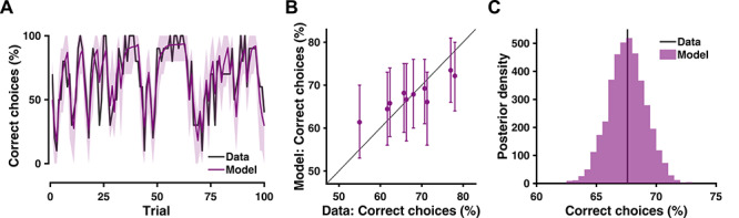
Model validation with posterior predictive check (PPC). (A) Trial-by-trial model predictions plotted against actual data. Shaded area depicts the 95% highest density interval (HDI) of the posterior distribution. (B) Individual’s model prediction compared with actual data, in relation to the identity line. Error bars depict the 95% HDI of the posterior distribution. (C) Grand average model prediction across trials and participants.

In the field of social neuroscience, only a handful of studies have so far employed PPC (e.g. Zhang and Gläscher, 2020; Lindström et al., 2019a; Lindström et al., 2019b). However, now that most cognitive models are constructed using mathematical operations, which entail the feature to generate new data, we strongly articulate that performing PPCs is indispensable when conducting computational modeling. This is especially true when Bayesian estimation is employed for fitting models (see the next section). Lacking such direct assessment between generated data and observed data might lead to less sound support of the associated cognitive processes, hence resulting in weaker implications when carrying out subsequent analyses.

Moving toward hierarchical model estimation

There are multiple ways to estimate the learning rate and the inverse temperature parameters in RL models, with some being more appropriate than others. Here, we describe why we advocate a hierarchical approach and provide several examples of toolboxes one can use to perform hierarchical modeling.

Typically, in a study, we are interested in the behavior of several subjects and possibly several groups of subjects (e.g. comparing clinical vs non-clinical populations or treatment vs control groups). The most straightforward approach is to assume that the parameters are fixed across subjects and estimate one set of parameters for the entire population. This, however, inevitably ignores the between-subject variability and could potentially lead to overstating the differences in parameter means between groups; hence, results from this approach are not generalizable to the population (Gelman et al., 2013; Maxwell et al., 2017; McElreath, 2018). A prevailing approach has therefore been to estimate a set of parameters for each subject separately (i.e. treating the parameters as random effects) and then use simple linear models (e.g. t-tests) to compare groups. The crucial problem of this method is that it tends to lead to extreme parameter values (e.g. unlikely low or high learning rates) and it inflates the population variance (Daw, 2011; Lebreton et al., 2019); thus, it is not well-suited for comparing group-level statistics.

It is therefore more accurate and stable to estimate both the individual and group level parameters simultaneously using hierarchical models (often interchangeable with multilevel model, mixed model, or partial pooling; Gelman et al., 2013; Maxwell et al., 2017; McElreath, 2018). The main benefit of this approach is that we pool data across individuals to explicitly estimate the mean and variance of the population. The group estimates then conversely constrains the parameter estimation of each individual in the group, thus avoiding unlikely extreme values. Although the advantages of hierarchical models have long been recognized (Lee, 2011; Bartlema et al., 2014; Lee and Wagenmakers, 2014; Ahn et al., 2017), it has until recently been computationally too demanding and complicated to perform. Advances in computing power and approximation methods have led to developments of readily available tools and packages that make these previously less accessible methods easy to use. These include the hBayesDM toolbox (Ahn et al., 2017), the VBA toolbox (Daunizeau et al., 2014), the HGF toolbox (Mathys et al., 2011; Mathys et al., 2014) in the TAPAS software collection (https://git.io/fjUn8), the HDDM toolbox (Wiecki et al., 2013), the MFIT toolbox (https://git.io/Je0jw) and the CBM toolbox (Piray et al., 2019a). All these toolboxes have optimized model specifications and considered proper parameter distributions. In fact, many of the toolboxes have already been used in social neuroscience (e.g. Fineberg et al., 2018; Hu et al., 2018; Zhang and Gläscher, 2020; see Supplementary Note 6 for statistical considerations for using hierarchical models to compare group differences; see also Valton et al., 2020 for a review), and following the workflow provided by these toolboxes is less prone to misspecification and misinterpretation (in the case of Type II error) when applying computational modeling.

Concluding summary

In the present work, we raise the awareness of common pitfalls of employing reinforcement learning (RL) in social neuroscience and give suggestions of best practices. This is to provide a set of guidelines to accurately interpret results and to improve scientific practice when using computational modeling. With the simple Rescorla–Wagner RL model as the example, we provide a principled and detailed interpretation of the learning rate using simulation, followed by the illustration of inspecting the theoretical subcomponents of the prediction error to justify its neural correlates. Finally, we address the necessity of validating models alongside model comparison. Besides, we illustrate the consideration of performing hierarchical modeling and direct readers to available toolboxes. Note that our suggestions (except for justifying the PE signal) are neither specific to reinforcement learning nor to social neuroscience. We recommend running simulations to gain a better comprehension of parameters for all kinds of computational models, and importantly, this can be accomplished even before data collection. Note that although RL models have been shown to be a powerful tool in social neuroscience, other forms of models are insightful as well. For example, the inequality aversion model has been employed to assess separate types of inequality aversion in economic games (Gao et al., 2018; Hu et al., 2018; van Baar et al., 2019); the Bayesian belief update model has been used to study moral decisions (Siegel et al., 2018, 2019); the interactive partially observable Markov decision process (i-POMDP) has been applied to examine higher-level theory of mind during strategic social interaction (Doshi et al., 2009; Hula et al., 2018; see Rusch et al., 2020 for a review). Even under the RL framework, other types of RL models, for example, the two-step RL model (Lockwood et al., 2019) and RL model with dynamic learning rate (Piray et al., 2019b), are also applied to a range of social learning paradigms. Discussing all above models, however, is beyond the scope of this paper; instead, listing them serves as a roadmap so that interested readers will know where to start when coming across these models in their own research.

To conclude, when handled properly, reinforcement learning models can uncover insightful cognitive processes that are otherwise intangible with classic approaches in social neuroscience. It is important to minimize misconception and misinterpretation when applying reinforcement learning models in social neuroscience. These suggestions are meant to aid future studies in interpreting and unpacking the neurocomputational mechanisms of social behaviors.

Data and software availability

Data and custom code to perform simulation and analysis can be accessed at the GitHub repository: https://github.com/lei-zhang/socialRL.

About the authors

L.Z. holds a PhD in cognitive neuroscience and is the co-developer of the hBayesDM package; L.L. is a PhD candidate, holds a master’s degree in psychology and has advanced training in statistics; N.M. is a PhD candidate and holds dual master’s degrees in cognitive science and in mathematics; J.G. is a principal investigator in computational neuroscience; and C.L. is a professor in social neuroscience.

Funding

This work was in part supported by the International Research Training Groups ‘CINACS’ (DFG GRK 1247), the Research Promotion Fund (FFM) for young scientists of the University Medical Center Hamburg-Eppendorf, National Natural Science Foundation of China (NSFC 71801110), the Ministry of Education in China Project of Humanities and Social Sciences (MOE 18YJC630268) and China Postdoctoral Science Foundation (No. 2018M633270) to L.Z.; the Bernstein Award for Computational Neuroscience (BMBF 01GQ1006), the Collaborative Research Center ‘Cross-modal learning’ (DFG TRR 169) and the Collaborative Research in Computational Neuroscience (CRCNS) grant (BMBF 01GQ1603) to J.G.; the Vienna Science and Technology Fund (WWTF VRG13-007) and Austrian Science Fund (FWF P 32686) to C.L.

Conflict of interest

The authors declare no competing financial interests.

References

- Ahn W.-Y., Haines N., Zhang L. (2017). Revealing neurocomputational mechanisms of reinforcement learning and decision-making with the hBayesDM package. Computational Psychiatry, 1, 24–57. [DOI] [PMC free article] [PubMed] [Google Scholar]
- Ashby F.G., Maddox W.T. (2011). Human category learning 2.0. Annals of the New York Academy of Sciences, 1224, 147–61. [DOI] [PMC free article] [PubMed] [Google Scholar]
- Aylward J., Valton V., Ahn W.-Y., et al. (2019). Altered learning under uncertainty in unmedicated mood and anxiety disorders. Nature Human Behaviour, 3, 1116–23. [DOI] [PMC free article] [PubMed] [Google Scholar]
- van Baar J.M., Chang L.J., Sanfey A.G. (2019). The computational and neural substrates of moral strategies in social decision-making. Nature Communications, 10, 1483. [DOI] [PMC free article] [PubMed] [Google Scholar]
- Bartlema A., Lee M., Wetzels R., Vanpaemel W. (2014). A Bayesian hierarchical mixture approach to individual differences: case studies in selective attention and representation in category learning. Journal of Mathematical Psychology, 59, 132–50. [Google Scholar]
- Behrens T.E.J., Woolrich M.W., Walton M.E., Rushworth M.F.S. (2007). Learning the value of information in an uncertain world. Nature Neuroscience, 10, 1214–21. [DOI] [PubMed] [Google Scholar]
- Behrens T.E.J., Hunt L.T., Woolrich M.W., Rushworth M.F.S. (2008). Associative learning of social value. Nature, 456, 245–9. [DOI] [PMC free article] [PubMed] [Google Scholar]
- Burke C.J., Tobler P.N., Baddeley M., Schultz W. (2010). Neural mechanisms of observational learning. Proceedings of the National Academy of Sciences of the United States of America, 107, 14431–6. [DOI] [PMC free article] [PubMed] [Google Scholar]
- Chien S., Wiehler A., Spezio M., Gläscher J. (2016). Congruence of inherent and acquired values facilitates reward-based decision-making. Journal of Neuroscience, 36, 5003–12. [DOI] [PMC free article] [PubMed] [Google Scholar]
- Cohen J.D., Daw N., Engelhardt B., et al. (2017). Computational approaches to fMRI analysis. Nature Neuroscience, 20, 304–13. [DOI] [PMC free article] [PubMed] [Google Scholar]
- Cools R., Altamirano L., D’Esposito M. (2006). Reversal learning in Parkinson’s disease depends on medication status and outcome valence. Neuropsychologia, 44, 1663–73. [DOI] [PubMed] [Google Scholar]
- Crawley D., Zhang L., Jones E., et al. (2019). Modeling cognitive flexibility in autism spectrum disorder and typical development reveals comparable developmental shifts in learning mechanisms. PsyArXiv. doi: 10.31234/osf.io/h7jcm. [DOI] [Google Scholar]
- Crockett M.J., Clark L., Tabibnia G., Lieberman M.D., Robbins T.W. (2008). Serotonin modulates behavioral reactions to unfairness. Science, 320, 1739. [DOI] [PMC free article] [PubMed] [Google Scholar]
- Crockett M.J., Clark L., Hauser M.D., Robbins T.W. (2010). Serotonin selectively influences moral judgment and behavior through effects on harm aversion. Proceedings of the National Academy of Sciences of the United States of America, 107, 17433–8. [DOI] [PMC free article] [PubMed] [Google Scholar]
- Daunizeau J., Adam V., Rigoux L. (2014). VBA: a probabilistic treatment of nonlinear models for neurobiological and behavioural data. PLoS Computational Biology, 10, e1003441. [DOI] [PMC free article] [PubMed] [Google Scholar]
- Daw N.D. (2011). Trial-by-trial Data Analysis using Computational Models. Decision Making, Affect, and Learning: Attention and Performance XXIII, pp. 1–26.
- Daw N.D. (2013). Advanced Reinforcement Learning. Neuroeconomics: Decision Making and the Brain, 2nd edn, pp. 299–320.
- Daw N.D., O’Doherty J.P., Dayan P., Seymour B., Dolan R.J. (2006). Cortical substrates for exploratory decisions in humans. Nature, 441, 876–9. [DOI] [PMC free article] [PubMed] [Google Scholar]
- Dolan R.J., Dayan P. (2013). Goals and habits in the brain. Neuron, 80, 312–25. [DOI] [PMC free article] [PubMed] [Google Scholar]
- Doshi P., Zeng Y., Chen Q. (2009). Graphical models for interactive POMDPs: representations and solutions. Autonomous Agents and Multi-Agent Systems, 18, 376–416. [Google Scholar]
- Eisenegger, C., Pedroni, A., Rieskamp, J., et al. (2013). DAT1 polymorphism determines L-DOPA effects on learning about others' prosociality. PLoS ONE, 8, e67820. [DOI] [PMC free article] [PubMed] [Google Scholar]
- Fineberg S.K., Leavitt J., Stahl D.S., et al. (2018). Differential valuation and learning from social and nonsocial cues in borderline personality disorder. Biological Psychiatry, 1–8. [DOI] [PMC free article] [PubMed] [Google Scholar]
- Forstmann B.U., Wagenmakers E.-J. (2015). An Introduction to Model-based Cognitive Neuroscience, New York, NY: Springer. [Google Scholar]
- Frank M.J., Moustafa A.A., Haughey H.M., Curran T., Hutchison K.E. (2007). Genetic triple dissociation reveals multiple roles for dopamine in reinforcement learning. Proceedings of the National Academy of Sciences, 104, 16311–6. [DOI] [PMC free article] [PubMed] [Google Scholar]
- Frank M.J., Gagne C., Nyhus E., et al. (2015). fMRI and EEG predictors of dynamic decision parameters during human reinforcement learning. Journal of Neuroscience, 35, 485–94. [DOI] [PMC free article] [PubMed] [Google Scholar]
- Friston K., Kiebel S. (2009). Predictive coding under the free-energy principle. Philosophical Transactions of the Royal Society, B: Biological Sciences, 364, 1211–21. [DOI] [PMC free article] [PubMed] [Google Scholar]
- Gao X., Yu H., Sáez I., et al. (2018). Distinguishing neural correlates of context-dependent advantageous- and disadvantageous-inequity aversion. Proceedings of the National Academy of Sciences of the United States of America, 115, E7680–9. [DOI] [PMC free article] [PubMed] [Google Scholar]
- Gelman A., Stern H.S., Carlin J.B., Stern H.S., Rubin D., Dunson D. (2013). Bayesian Data Analysis, Boca Raton, FL: Chapman and Hall/CRC. [Google Scholar]
- Gläscher J., O’Doherty J.P. (2010). Model-based approaches to neuroimaging: combining reinforcement learning theory with fMRI data. Wiley Interdisciplinary Reviews: Cognitive Science, 1, 501–10. [DOI] [PubMed] [Google Scholar]
- Gläscher J., Hampton A.N., O’Doherty J.P. (2009). Determining a role for ventromedial prefrontal cortex in encoding action-based value signals during reward-related decision making. Cerebral Cortex, 19, 483–95. [DOI] [PMC free article] [PubMed] [Google Scholar]
- Gläscher J., Daw N., Dayan P., O’Doherty J.P. (2010). States versus rewards: dissociable neural prediction error signals underlying model-based and model-free reinforcement learning. Neuron, 66, 585–95. [DOI] [PMC free article] [PubMed] [Google Scholar]
- Guitart-Masip M., Fuentemilla L., Bach D.R., et al. (2011). Action dominates valence in anticipatory representations in the human striatum and dopaminergic midbrain. Journal of Neuroscience, 31, 7867–75. [DOI] [PMC free article] [PubMed] [Google Scholar]
- Haines N., Vassileva J., Ahn W.Y. (2018). The outcome-representation learning model: a novel reinforcement learning model of the Iowa gambling task. Cognitive Science, 42, 2534–61. [DOI] [PMC free article] [PubMed] [Google Scholar]
- Hampton A.N., Bossaerts P., O’Doherty J.P. (2008). Neural correlates of mentalizing-related computations during strategic interactions in humans. Proceedings of the National Academy of Sciences of the United States of America, 105, 6741–6. [DOI] [PMC free article] [PubMed] [Google Scholar]
- Hauser T.U., Iannaccone R., Walitza S., Brandeis D., Brem S. (2015). Cognitive flexibility in adolescence: neural and behavioral mechanisms of reward prediction error processing in adaptive decision making during development. NeuroImage, 104, 347–54. [DOI] [PMC free article] [PubMed] [Google Scholar]
- Hill C.A., Suzuki S., Polania R., Moisa M., O'Doherty J.P., Ruff C.C. (2017). A causal account of the brain network computations underlying strategic social behavior. Nature Neuroscience, 20, 1142–9. [DOI] [PubMed] [Google Scholar]
- Hu Y., He L., Zhang L., Wölk T., Dreher J.-C., Weber B. (2018). Spreading inequality: neural computations underlying paying-it-forward reciprocity. Social Cognitive and Affective Neuroscience, 13, 578–89. [DOI] [PMC free article] [PubMed] [Google Scholar]
- Hula A., Vilares I., Lohrenz T., Dayan P., Montague P.R. (2018). A model of risk and mental state shifts during social interaction. PLoS Computational Biology, 14, 1–20. [DOI] [PMC free article] [PubMed] [Google Scholar]
- Ihssen N., Mussweiler T., Linden D.E.J. (2016). Observing others stay or switch—how social prediction errors are integrated into reward reversal learning. Cognition, 153, 19–32. [DOI] [PubMed] [Google Scholar]
- Jocham G., Furlong P.M., Kröger I.L., Kahn M.C., Hunt L.T., Behrens T.E.J. (2014). Dissociable contributions of ventromedial prefrontal and posterior parietal cortex to value-guided choice. NeuroImage, 100, 498–506. [DOI] [PMC free article] [PubMed] [Google Scholar]
- Jones R.M., Somerville L.H., Li J., et al. (2014). Adolescent-specific patterns of behavior and neural activity during social reinforcement learning. Cognitive, Affective, & Behavioral Neuroscience, 14, 683–97. [DOI] [PMC free article] [PubMed] [Google Scholar]
- Klein T.A., Ullsperger M., Jocham G. (2017). Learning relative values in the striatum induces violations of normative decision making. Nature Communications, 8, 1–12. [DOI] [PMC free article] [PubMed] [Google Scholar]
- Klucharev V., Hytönen K., Rijpkema M., Smidts A., Fernández G. (2009). Reinforcement learning signal predicts social conformity. Neuron, 61, 140–51. [DOI] [PubMed] [Google Scholar]
- Koizumi A., Amano K., Cortese A., et al. (2017). Fear reduction without fear through reinforcement of neural activity that bypasses conscious exposure. Nature Human Behaviour, 1, 1–7. [DOI] [PMC free article] [PubMed] [Google Scholar]
- Konovalov A., Hu J., Ruff C.C. (2018). Neurocomputational approaches to social behavior. Current Opinion in Psychology, 24, 41–7. [DOI] [PubMed] [Google Scholar]
- Korn C.W., Bach D.R. (2018). Heuristic and optimal policy computations in the human brain during sequential decision-making. Nature Communications, 9, 325. [DOI] [PMC free article] [PubMed] [Google Scholar]
- Lebreton M., Bavard S., Daunizeau J., et al. (2019). Assessing inter-individual differences with task-related functional neuroimaging. Nature Human Behaviour, 3, 897–5. [DOI] [PubMed] [Google Scholar]
- Lee M.D. (2011). How cognitive modeling can benefit from hierarchical Bayesian models. Journal of Mathematical Psychology, 55, 1–7. [Google Scholar]
- Lee M.D., Wagenmakers E.-J. (2014). Bayesian Cognitive Modeling: A Practical Course, Cambridge: Cambridge University Press. [Google Scholar]
- Lee D., Seo H., Jung M.W. (2012). Neural basis of reinforcement learning and decision making. Annual Review of Neuroscience, 35, 287–308. [DOI] [PMC free article] [PubMed] [Google Scholar]
- Levy R., Mislevy R.J., Sinharay S. (2009). Posterior predictive model checking for multidimensionality in item response theory. Applied Psychological Measurement, 33, 519–37. [Google Scholar]
- Lewandowsky S., Farrell S. (2010). Computational Modeling in Cognition: Principles and Practice, Thousand Oaks, CA: SAGE Publications. [Google Scholar]
- Li J., Schiller D., Schoenbaum G., Phelps E.A., Daw N.D. (2011). Differential roles of human striatum and amygdala in associative learning. Nature Neuroscience, 14, 1250–2. [DOI] [PMC free article] [PubMed] [Google Scholar]
- Lin A., Rangel A., Adolphs R. (2012). Impaired learning of social compared to monetary rewards in autism. Frontiers in Neuroscience, 6, 1–7. [DOI] [PMC free article] [PubMed] [Google Scholar]
- Lindström B., Haaker J., Olsson A. (2018). A common neural network differentially mediates direct and social fear learning. NeuroImage, 167, 121–9. [DOI] [PubMed] [Google Scholar]
- Lindström B., Bellander M., Chang A., Tobler P.N., Amodio D.M. (2019a). A computational reinforcement learning account of social media engagement. PsyArXiv. doi: 10.31234/osf.io/78mh5. [DOI] [Google Scholar]
- Lindström B., Golkar A., Jangard S., Tobler P.N., Olsson A. (2019b). Social threat learning transfers to decision making in humans. Proceedings of the National Academy of Sciences of the United States of America, 116, 4732–7. [DOI] [PMC free article] [PubMed] [Google Scholar]
- Lockwood P.L., Klein-Flügge M.C. (2020). Computational modelling of social cognition and behaviour—a reinforcement learning primer. Social Cognitive and Affective Neuroscience, 1–11. [DOI] [PMC free article] [PubMed] [Google Scholar]
- Lockwood P.L., Wittmann M.K. (2018). Ventral anterior cingulate cortex and social decision-making. Neuroscience and Biobehavioral Reviews, 92, 187–91. [DOI] [PMC free article] [PubMed] [Google Scholar]
- Lockwood P.L., Apps M.A.J., Valton V., Viding E., Roiser J.P. (2016). Neurocomputational mechanisms of prosocial learning and links to empathy. Proceedings of the National Academy of Sciences, 113, 9763–8. [DOI] [PMC free article] [PubMed] [Google Scholar]
- Lockwood P.L., Wittmann M.K., Apps M.A.J., et al. (2018). Neural mechanisms for learning self and other ownership. Nature Communications, 9, 4747. [DOI] [PMC free article] [PubMed] [Google Scholar]
- Lockwood P.L., Klein-flügge M., Abdurahman A., Crockett M.J. (2019). Neural signatures of model-free learning when avoiding harm to self and other. bioRxiv, 718106. [Google Scholar]
- Lynch S.M., Western B. (2004). Bayesian posterior predictive checks for complex models. Sociological Methods & Research, 32, 301–35. [Google Scholar]
- Mathys C., Daunizeau J., Friston K.J., Stephan K.E. (2011). A Bayesian foundation for individual learning under uncertainty. Frontiers in Human Neuroscience, 5, 9. [DOI] [PMC free article] [PubMed] [Google Scholar]
- Mathys C., Lomakina E.I., Daunizeau J., et al. (2014). Uncertainty in perception and the hierarchical Gaussian filter. Frontiers in Human Neuroscience, 8, 1–24. [DOI] [PMC free article] [PubMed] [Google Scholar]
- Maxwell S.E., Delaney H.D., Kelley K. (2017). Designing Experiments and Analyzing Data: A Model Comparison Perspective, New York, NY: Routledge. [Google Scholar]
- McElreath R. (2018). Statistical Rethinking: A Bayesian Course with Examples in R and Stan, Boca Raton, FL: Chapman and Hall/CRC. [Google Scholar]
- Melinscak F., Bach D.R. (2020). Computational optimization of associative learning experiments. PLoS Computational Biology, 16, 1–23. [DOI] [PMC free article] [PubMed] [Google Scholar]
- Niv Y., Edlund J.A., Dayan P., O'Doherty J.P. (2012). Neural prediction errors reveal a risk-sensitive reinforcement-learning process in the human brain. Journal of Neuroscience, 32, 551–62. [DOI] [PMC free article] [PubMed] [Google Scholar]
- Norbury A., Robbins T.W., Seymour B. (2018). Value generalization in human avoidance learning. eLife, 7, 1–30. [DOI] [PMC free article] [PubMed] [Google Scholar]
- O’Doherty J.P., Dayan P., Friston K., Critchley H., Dolan R.J. (2003). Temporal difference models and reward-related learning in the human brain. Neuron, 38, 329–37. [DOI] [PubMed] [Google Scholar]
- O’Doherty J.P., Dayan P., Schultz J., Deichmann R., Friston K., Dolan R.J. (2004). Dissociable roles of ventral and dorsal striatum in instrumental conditioning. Science, 304, 452–4. [DOI] [PubMed] [Google Scholar]
- O’Doherty J.P., Hampton A., Kim H. (2007). Model-based fMRI and its application to reward learning and decision making. Annals of the New York Academy of Sciences, 1104, 35–53. [DOI] [PubMed] [Google Scholar]
- O’Doherty J.P., Cockburn J., Pauli W.M. (2017). Learning, reward, and decision making. Annual Review of Psychology, 68, 73–100. [DOI] [PMC free article] [PubMed] [Google Scholar]
- Olsson A., Knapska E., Lindström B. (2020). The neural and computational systems of social learning. Nature Reviews Neuroscience, 21, 197–212. [DOI] [PubMed] [Google Scholar]
- den Ouden H.E.M., Daw N.D., Fernández G., et al. (2013). Supplement: dissociable effects of dopamine and serotonin on reversal learning. Neuron, 80, 1090–100. [DOI] [PubMed] [Google Scholar]
- Pagnoni G., Zink C.F., Montague P.R., Berns G.S. (2002). Activity in human ventral striatum locked to errors of reward prediction. Nature Neuroscience, 5, 97–8. [DOI] [PubMed] [Google Scholar]
- Palminteri S., Wyart V., Koechlin E. (2017). The importance of falsification in computational cognitive modeling. Trends in Cognitive Sciences, 21, 425–33. [DOI] [PubMed] [Google Scholar]
- Pessiglione M., Seymour B., Flandin G., Dolan R.J., Frith C.D. (2006). Dopamine-dependent prediction errors underpin reward-seeking behaviour in humans. Nature, 442, 1042–5. [DOI] [PMC free article] [PubMed] [Google Scholar]
- Piray P., Dezfouli A., Heskes T., Frank M.J., Daw N.D. (2019a). Hierarchical Bayesian inference for concurrent model fitting and comparison for group studies. PLoS Computational Biology, 15, e1007043. [DOI] [PMC free article] [PubMed] [Google Scholar]
- Piray P., Ly V., Roelofs K., Cools R., Toni I. (2019b). Emotionally aversive cues suppress neural systems underlying optimal learning in socially anxious individuals. The Journal of Neuroscience, 39, 1445–56. [DOI] [PMC free article] [PubMed] [Google Scholar]
- Poldrack R.A., Foerde K. (2008). Category learning and the memory systems debate. Neuroscience and Biobehavioral Reviews, 32, 197–205. [DOI] [PubMed] [Google Scholar]
- Rangel A., Camerer C., Montague P.R. (2008). A framework for studying the neurobiology of value-based decision making. Nature Reviews Neuroscience, 9, 545–56. [DOI] [PMC free article] [PubMed] [Google Scholar]
- Ratcliff R., McKoon G. (2008). The diffusion decision model: theory and data for two-choice decision tasks. Neural Computation, 20, 873–922. [DOI] [PMC free article] [PubMed] [Google Scholar]
- Rescorla R.A., Wagner A.R. (1972). A theory of Pavlovian conditioning: Variations in the effectiveness of reinforcement and nonreinforcement In: Classical Conditioning II: Current Research and Theory, New York, NY: Appleton-Century-Crofts, Vol. 2, pp. 64–99. [Google Scholar]
- Roy M., Shohamy D., Daw N., Jepma M., Wimmer G.E., Wager T.D. (2014). Representation of aversive prediction errors in the human periaqueductal gray. Nature Neuroscience, 17, 1607–12. [DOI] [PMC free article] [PubMed] [Google Scholar]
- Ruff C.C., Fehr E. (2014). The neurobiology of rewards and values in social decision making. Nature Reviews Neuroscience, 15, 549–62. [DOI] [PubMed] [Google Scholar]
- Rusch T., Steixner-Kumar S., Doshi P., Spezio M., Gläscher J. (2020). Theory of mind and decision science: towards a typology of tasks and computational models. Neuropsychologia, 146, 107488. [DOI] [PubMed] [Google Scholar]
- Sakamoto, Y., Ishiguro, M., Kitagawa, G. (1986). Akaike information criterion statistics, 81. Taylor & Francis. [Google Scholar]
- Seid-Fatemi A., Tobler P.N. (2015). Efficient learning mechanisms hold in the social domain and are implemented in the medial prefrontal cortex. Social Cognitive and Affective Neuroscience, 10, 735–43. [DOI] [PMC free article] [PubMed] [Google Scholar]
- Siegel J.Z., Mathys C., Rutledge R.B., Crockett M.J. (2018). Beliefs about bad people are volatile. Nature Human Behaviour, 2, 750–6. [DOI] [PubMed] [Google Scholar]
- Siegel J.Z., Estrada S., Crockett M.J., et al. (2019). Exposure to violence affects the development of moral impressions and trust behavior in incarcerated males. Nature Communications, 10, 1–9. [DOI] [PMC free article] [PubMed] [Google Scholar]
- Simmons J.P., Nelson L.D., Simonsohn U. (2011). False-positive psychology: undisclosed flexibility in data collection and analysis allows presenting anything as significant. Psychological Science, 22, 1359–66. [DOI] [PubMed] [Google Scholar]
- Soltani A., Izquierdo A. (2019). Adaptive learning under expected and unexpected uncertainty. Nature Reviews Neuroscience, 20, 635–44. [DOI] [PMC free article] [PubMed] [Google Scholar]
- Steingroever H., Wetzels R., Wagenmakers E.J. (2013). Validating the PVL-Delta model for the Iowa gambling task. Frontiers in Psychology, 4, 1–17. [DOI] [PMC free article] [PubMed] [Google Scholar]
- Steingroever H., Wetzels R., Wagenmakers E.J. (2014). Absolute performance of reinforcement-learning models for the Iowa gambling task. Decision, 1, 161–83. [Google Scholar]
- Sun S., Yu R. (2014). The feedback related negativity encodes both social rejection and explicit social expectancy violation. Frontiers in Human Neuroscience, 8, 1–9. [DOI] [PMC free article] [PubMed] [Google Scholar]
- Sutton R.S., Barto A.G. (1981). Toward a modern theory of adaptive networks: expectation and prediction. Psychological Review, 88, 135–70. [PubMed] [Google Scholar]
- Sutton R.S., Barto A.G. (2018). Reinforcement Learning: An Introduction, Cambridge, MA: MIT Press Cambridge. [Google Scholar]
- Suzuki S., Harasawa N., Ueno K., et al. (2012). Learning to simulate others’ decisions. Neuron, 74, 1125–37. [DOI] [PubMed] [Google Scholar]
- Swart J.C., Froböse M.I., Cook J.L., et al. (2017). Catecholaminergic challenge uncovers distinct Pavlovian and instrumental mechanisms of motivated (in)action. eLife, 6, 1–36. [DOI] [PMC free article] [PubMed] [Google Scholar]
- Thorndike E.L. (1927). The law of effect. The American Journal of Psychology, 39, 212. [Google Scholar]
- Tzovara A., Korn C.W., Bach D.R. (2018). Human Pavlovian fear conditioning conforms to probabilistic learning. PLoS Computational Biology, 14, e1006243. [DOI] [PMC free article] [PubMed] [Google Scholar]
- Valton V., Wise T., Robinson O.J. (2020). The importance of group specification in computational modelling of behaviour. PsyArXiv. doi: 10.31234/osf.io/p7n3h. [DOI] [Google Scholar]
- Vehtari A., Gelman A., Gabry J. (2016). Practical Bayesian model evaluation using leave-one-out cross-validation and WAIC. Statistics and Computing, 27, 1–20. [Google Scholar]
- Wicherts J.M., Veldkamp C.L.S., Augusteijn H.E.M., Bakker M., van Aert R.C.M., van Assen M.A.L.M. (2016). Degrees of freedom in planning, running, analyzing, and reporting psychological studies: a checklist to avoid P-hacking. Frontiers in Psychology, 7, 1–12. [DOI] [PMC free article] [PubMed] [Google Scholar]
- Wiecki T.V., Sofer I., Frank M.J. (2013). HDDM: hierarchical Bayesian estimation of the drift-diffusion model in python. Frontiers in Neuroinformatics, 7, 1–10. [DOI] [PMC free article] [PubMed] [Google Scholar]
- Will G.-J., Rutledge R.B., Moutoussis M., Dolan R.J. (2017). Neural and computational processes underlying dynamic changes in self-esteem. eLife, 6, e28098. [DOI] [PMC free article] [PubMed] [Google Scholar]
- Wilson R.C., Collins A.G. (2019). Ten simple rules for the computational modeling of behavioral data. eLife, 8, 1–35. [DOI] [PMC free article] [PubMed] [Google Scholar]
- Wilson R.C., Niv Y. (2015). Is model fitting necessary for model-based fMRI? PLoS Computational Biology, 11, 1–21. [DOI] [PMC free article] [PubMed] [Google Scholar]
- Yoon L., Somerville L.H., Kim H. (2018). Development of MPFC function mediates shifts in self-protective behavior provoked by social feedback. Nature Communications, 9, 1–10. [DOI] [PMC free article] [PubMed] [Google Scholar]
- Zhang L., Gläscher J. (2020). A brain network supporting social influences in human decision-making. Science Advances, in press. [DOI] [PMC free article] [PubMed] [Google Scholar]
- Zhu L., Mathewson K.E., Hsu M. (2012). Dissociable neural representations of reinforcement and belief prediction errors underlie strategic learning. Proceedings of the National Academy of Sciences, 109, 1419–24. [DOI] [PMC free article] [PubMed] [Google Scholar]
Associated Data
This section collects any data citations, data availability statements, or supplementary materials included in this article.
Supplementary Materials
Data Availability Statement