Bayesian-based predictions of COVID-19 evolution in Texas using multispecies mixture-theoretic continuum models

Abstract

We consider a mixture-theoretic continuum model of the spread of COVID-19 in Texas. The model consists of multiple coupled partial differential reaction–diffusion equations governing the evolution of susceptible, exposed, infectious, recovered, and deceased fractions of the total population in a given region. We consider the problem of model calibration, validation, and prediction following a Bayesian learning approach implemented in OPAL (the Occam Plausibility Algorithm). Our goal is to incorporate COVID-19 data to calibrate the model in real-time and make meaningful predictions and specify the confidence level in the prediction by quantifying the uncertainty in key quantities of interests. Our results show smaller mortality rates in Texas than what is reported in the literature. We predict 7003 deceased cases by September 1, 2020 in Texas with $95\%$ CI 6802–7204. The model is validated for the total deceased cases, however, is found to be invalid for the total infected cases. We discuss possible improvements of the model.

Introduction

Modeling the spreading of infectious diseases can help in extracting relevant information from the data, such as effective reproduction rates, mortality rates, contact rates, in exploring the effectiveness of various preventive measures and their effect on the epidemic, developing a deeper understanding of how the particular disease spreads and major features that support the spreading, [15]. During 2020, much of the world has been under lockdown due to a novel SARS-CoV-2 virus. The virus originated in Wuhan, China, and has resulted in the loss of many lives, loss of livelihood, and almost complete shutdown of economies. SARS-CoV-2 virus infection spreads via droplets generated during coughing/sneezing and touching contaminated surfaces. To slow down its spread, people are advised to maintain social distancing and in certain places even strict restriction on public movement is enforced. The virus seem to infect all groups, however, has been more deadly for older people and people with compromised immunity [8, 9, 18, 28]. While the search for vaccines and drugs are going on, the researchers across the globe have put in an effort to develop a model that captures the evolution of the epidemic and reveal the important parameters which help policy makers and medical professionals in devising preventive strategies.

Existing works on COVID-19 epidemic prediction include stochastic transmission models (compartmental models) based on the idea of putting individuals in different categories, such as susceptible (S), exposed (E), infected (I), recovered/removed (R), and deceased (D). Each category evolves in time often captured by systems of ODEs and are coupled to other species through the cross-interaction terms. These models average the individual interaction and therefore are more effective for large-scale epidemics. Such models have been applied to extract the relevant information such as the effective reproduction rate (number of secondary infections at given time) [2, 17], account for asymptotic cases on disease spread [26], and to test the effects of preventive measures such as social distancing and isolation [14]. The parameters in the cross-interaction terms can be either assumed to be constant in time or time varying to include the effect of various preventive policies such as social-distancing, strict isolation directives, in the model [10, 17]. Compartmental models can be generalized by allowing fields corresponding to each category to vary in space. The random (Brownian) motion of individuals is approximated by diffusion term whereas the interaction between categories is modeled by reaction terms, [16]. This results in a set of nonlinearly coupled reaction–diffusion PDEs (partial differential equations). Recently a model of this type has been applied to predict the spread of disease in Lombardy, Italy [30]. That work is based on the earlier model of the spread of rabies [16].

In this work, we consider a multi-species model of the evolution of COVID-19 which is characterized by a system of PDEs. The species comprise of the fractions of the population in the following categories: exposed but no symptoms, already infected, recovered after an infection, and those who succumbed to the virus. These fractions are treated as a continuous fields over a bounded domain in ${\mathbb{R}}^2$ (the state of Texas). The model considered in this work is inspired from the recent work [30] and earlier work [16].

The goal of this work is to apply a Bayesian learning in OPAL to model calibration, validation and prediction utilizing the spatially and temporally resolved data and to address uncertainties. We adopt the OPAL (Occam Plausibility Algorithm [11, 23, 24]) that is developed to deliver a systematic path toward valid prediction in the presence of uncertainties. Depending on the spatial resolution of interest (such as county, state, country), the data are available in real time listing the number of COVID-19 cases, number of recovered patients, number of patients deceased. An objective of this work is to leverage the data for model calibration and validation. Since the data are evolving, it is also necessary to evolve the model parameters (i.e. continuously update the model parameters over specified time intervals).

Bayesian learning consists of three key steps: calibration, validation, and prediction. In the calibration step, the model parameters are sampled through some assumed probability density function and, with an appropriate likelihood function, the probability densities (posteriors) of parameters are determined. This is the step where the data is sampled to obtain the pdf (probability distribution function) of model parameters. In the validation step, the model output is compared with the data and if the error is within a preset tolerance, the model is specified as Not Invalid. It can be noted that the calibration and validation steps are similar to the training and testing step in a deep learning framework; however, there is one important difference: in this Bayesian method, parameters are updated in the validation step as well. In all of the Bayesian steps, the likelihood function plays the key role. It assigns a penalty when the model output does not agree with the data. This is similar to the loss function in deep learning.

COVID-19 cases in Texas were initially slowly growing (period March 15–May 31). Near the end of May, the cases started rising rapidly. The jump in cases can be attributed to 1) opening up of businesses and less restriction in movement of people post May 20, and 2) the increase in COVID-19 testing resulting in large numbers of infected cases which may have gone unnoticed for mild cases otherwise. For our analysis, we consider the period June 1–June 30 as in this period the government policy remained somewhat the same making the assumption of temporally constant parameters less error-prone. We consider June 1–June 20 data for the calibration and June 21–June 30 for the validation of the model. Based on calibrated and validated model, we predict the total number of infected and deceased cases in 25 districts of Texas in the period July 1–September 1. It is shown that care is required in setting up a good model and scenario of prediction. Sensitivity analysis plays an important role in the model inference. For example, we show that when some of the model parameters were fixed to the values reported in previous studies, specifically the fatality rate (change from infected to deceased) and recovery rates (from infected to recovered), the total deceased cases will be insensitive to any change in parameters. The total deceased cases was mainly sensitive to the parameters described above and, by fixing them, we lose the ability to train our model. This also explains why in [30] authors saw large numbers of infected cases when they were trying to match the total deceased cases with data. Since the most sensitive parameters affecting total deceased cases was fixed in their study, they over estimate the infected cases to match the total deceased cases. Another important point emerging from our study is the sensitivity of the model output on the initial condition.

Results of the calibrated-validated model show a decrease in mortality rates for Texas as compared to mortality rates reported in literature [30]. Validation results show that the model parameters affecting total infected cases gets updated significantly, and, therefore, the total infected cases QoI computed from the validation posterior and calibration posterior show noticeable differences. This, we think, is natural as the number of infected cases is changing rapidly and the model is inadequate to accommodate this. Whereas, the total deceased cases QoI computed from the validation posterior and calibration posterior are close and we see small update of the parameters affecting the total deceased cases in the validation step. This suggests that the deceased cases in Texas has stabilized. We place higher confidence in our prediction of deceased cases. On June 30, 2020, there was total 2525 fatalities and total 175,977 infected cases all over Texas. We predict 7003 deceased cases and 301,658 infected cases by September 1, 2020 with uncertainty (standard deviation) 102 and 5786 respectively. The $95\%$ CI are 6802–7204 for deceased cases and 290,251–313,064 for infected cases.

The remainder of this paper is organized as follows: in Sect. 2, we describe the forward model. In Sect. 3, Bayesian approach in OPAL and associated components are presented. The discretization of the forward model, source and processing of the data and map are described in Sect. 4. Therein, we also present the sensitivity analysis results. In Sect. 5, we apply the Bayesian inference and show calibration-validation-prediction results. We discuss the prediction results and further improvements of the model in Sect.  6. We make the codes available publicly in website https://github.com/prashjha/BayesForSEIRD.

Reaction–diffusion model

Let $\mathrm{\Omega }\subset {\mathbb{R}}^2$ be a simply-connected geographical region projected on a 2D plane. Let [0, T] be the time domain of interest. At any point $\mathit{x}\in \mathrm{\Omega }$ and time $t\in [0,T]$, we introduce following real-valued fields:

• ${\varphi }_s={\varphi }_s(\mathit{x},t)$—susceptible population density (those not yet infected by COVID-19)

• ${\varphi }_e={\varphi }_e(\mathit{x},t)$—exposed population density (which are exposed but do not yet show symptoms)

• ${\varphi }_i={\varphi }_i(\mathit{x},t)$—infected population density

• ${\varphi }_r={\varphi }_r(\mathit{x},t)$—recovered population density

• ${\varphi }_d={\varphi }_d(\mathit{x},t)$—deceased population density

• ${\varphi }_n={\varphi }_n(\mathit{x},t)$—total population density

We have ${\varphi }_n={\varphi }_s+{\varphi }_e+{\varphi }_i+{\varphi }_r+{\varphi }_d$. By population density, of course, we mean the number of individuals per unit area in $\mathrm{\Omega }$. We assume ${\varphi }_n(\mathit{x},t)>0$ for all $(\mathit{x},t)\in \mathrm{\Omega }\times [0,T]$.

Fig. 1.

Schematics of SEIRD model with 5 compartments

Assuming sufficient smoothness and differentiability, the density fields are governed by the following nonlinear coupled system of PDEs:

$$\begin{array}{cc}\hfill {\partial }_t{\varphi }_s& =\alpha {\varphi }_n-\left(1,-,\frac{A}{{\varphi }_n}\right){\beta }_i{\varphi }_s{\varphi }_i-\left(1,-,\frac{A}{{\varphi }_n}\right){\beta }_e{\varphi }_s{\varphi }_e\hfill \\ \hfill & -\mu {\varphi }_s{\varphi }_n+\mathrm{\nabla }·({\varphi }_n{\nu }_s\mathrm{\nabla }{\varphi }_s),\hfill \\ \hfill {\partial }_t{\varphi }_e& =\left(1,-,\frac{A}{{\varphi }_n}\right){\beta }_i{\varphi }_s{\varphi }_i+\left(1,-,\frac{A}{{\varphi }_n}\right){\beta }_e{\varphi }_s{\varphi }_e-\sigma {\varphi }_e\hfill \\ \hfill & -{\gamma }_e{\varphi }_e-\mu {\varphi }_e{\varphi }_n+\mathrm{\nabla }·({\varphi }_n{\nu }_e\mathrm{\nabla }{\varphi }_e),\hfill \\ \hfill {\partial }_t{\varphi }_i& =\sigma {\varphi }_e-{\gamma }_d{\varphi }_i-{\gamma }_r{\varphi }_i-\mu {\varphi }_i{\varphi }_n+\mathrm{\nabla }·({\varphi }_n{\nu }_i\mathrm{\nabla }{\varphi }_i),\hfill \\ \hfill {\partial }_t{\varphi }_r& ={\gamma }_r{\varphi }_i+{\gamma }_e{\varphi }_e-\mu {\varphi }_r{\varphi }_n+\mathrm{\nabla }·({\varphi }_n{\nu }_r\mathrm{\nabla }{\varphi }_r),\hfill \\ \hfill {\partial }_t{\varphi }_d& ={\gamma }_d{\varphi }_i,\hfill \end{array}$$ 1

where ${\gamma }_a,a\in \{e,r\},$ are recovery rates, ${\gamma }_d$ is the mortality rate of COVID-19 infected patients, ${\beta }_a,a\in \{e,i\},$ are contact rates, ${\nu }_a,a\in \{s,e,i,r\},$ are diffusivity constants of various densities, $\alpha$ is the birth rate, $\sigma$ is the inverse of the incubation period, $\mu$ is the general mortality rate (non COVID-19), and A is the constant appearing due to Allee effect. Above model is based on commonly accepted physical processes, see [15]. Boundary conditions for fields are taken as Neumann conditions:

$$\begin{array}{c}\hfill \mathrm{\nabla }{\varphi }_a·\mathit{n}=0,\forall (\mathit{x},t)\in \Omega \times [0,T],\forall a\in \{s,e,i,r,d\}.\end{array}$$ 2

Initial conditions are given by

$$\begin{array}{c}\hfill {\varphi }_a(\mathit{x},0)={\varphi }_a^0(\mathit{x}),\forall \mathit{x}\in \Omega ,\forall a\in \{s,e,i,r,d\}.\end{array}$$ 3

We ignore natural death and birth i.e. $\alpha =\mu =0$. We remark that designing initial condition for this model is bit more involved and we discuss this in some detail in Sect. 4. Initially we have the data for the total infected cases (sum of infected, recovered, and deceased), deceased cases, recovered cases, and total population. To obtain the remaining fields, namely, exposed cases and susceptible cases, we assume that at $t=0$, there is a real number R such that

$$\begin{array}{c}\hfill {\varphi }_e(\mathit{x},0)=R{\varphi }_i(\mathit{x},0).\end{array}$$ 4

Calculations show that the model output can be sensitive to the choice of R. We add it to our list of model parameters to be determined by Bayesian inference.

Bayesian learning

Suppose the SEIRD (susceptible-exposed-infected-recovered-deceased) model in (1) can be expressed concisely as

$$\begin{array}{c}\hfill \mathcal{A}(\mathit{\theta },S;\mathit{u}(\mathit{\theta },S))=0,\end{array}$$ 5

where $\mathit{\theta }=(A,{\beta }_e,{\nu }_s,{\nu }_i,{\gamma }_e,{\gamma }_r,{\gamma }_d,\sigma ,R)\in \mathrm{\Theta }\subset {[0,\infty )}^{N_{\theta }}$, $N_{\theta }=9$, is the model parameter vector, S a scenario specifying the conditions on which the problem is posed, and $\mathit{u}(\mathit{\theta },S)=({\varphi }_s,{\varphi }_e,{\varphi }_i,{\varphi }_r,{\varphi }_d)$ is the vector of population densities satisfying the forward problem for a given parameter $\mathit{\theta }$ and scenario S. We assume that ${\beta }_i={\beta }_e$ and ${\nu }_r={\nu }_e={\nu }_s$ in rest of the article. This reduces the computational complexity of the model inference problem at a very little cost of approximation.

We assume that the solution $\mathit{u}(\mathit{\theta },S)$ belongs to the space ${[L^2(0,T;H^1(\mathrm{\Omega }))]}^5$, i.e., for each $a\in \{s,e,i,r,d\}$, the components of $\mathit{u}$ satisfy

$$\begin{array}{c}\hfill {\int }_0^T||{\varphi }_a{||}_1^2<\infty ,\end{array}$$ 6

where

$$\begin{array}{c}\hfill ||{\varphi }_a{||}_1={\left({\int }_{\mathrm{\Omega }},|,{\varphi }_a,{|}^2,+,{|\mathrm{\nabla }{\varphi }_a|}^2,d,\mathit{x}\right)}^{1/2}\end{array}$$ 7

is the $H^1$ Hilbert space norm. For simplicity, we let V denote the solution space, where

$$\begin{array}{c}\hfill V={[L^2(0,T;H^1(\mathrm{\Omega }))]}^5.\end{array}$$ 8

In the rest of the article, we will assume that for any $\mathit{\theta }\in \mathrm{\Theta }$ and given scenario S, the solution $\mathit{u}=\mathit{u}(\mathit{\theta },S)$ of the forward problem (5) exists and belongs to the space V.

While the solution of (5) describes the distribution of the disease over the total geographical region of the state of Texas, we are ultimately interested in the specific quantities computed from the solution $\mathit{u}$, such as the total number of cases of infected and deceased patients in each of a set of 25 districts into which the state is partitioned. The quantity of interest Q (QoI or QoIs when more than one quantity of interest) is a functional defined on the space of solutions of forward model, i.e.,

$$\begin{array}{c}\hfill Q:V\to \mathbb{R};Q(\mathit{u}(\mathit{\theta },S_p))=\tilde{Q}(\mathit{\theta }),\end{array}$$ 9

where $S_p$ is the prediction scenario, see [23, 24]. $\tilde{Q}$ is the random function since $\mathit{\theta }$ is a random variable. For the problem at hand, we consider the total cases of infected and deceased patients in each of 25 districts of Texas at prediction time $t=T_p$ as the QoIs.

Before we describe the three key steps in OPAL Bayesian learning, it is important to first discuss the various components of the approach.

Noise in the data and the model inadequacy

Experimental noise

Suppose g is the real data (the ground truth), $\mathit{Y}$ is the recorded data with some margin of error, and $ϵ$ is the noise, then $\mathit{Y}$ must be related to g by some function f (unknown)

$$\begin{array}{c}\hfill \mathit{Y}=f(g,ϵ).\end{array}$$

To proceed further, we need to assume some reasonable form of function f. Following common assumptions, we suppose that $ϵ$ follows the Gaussian distribution with mean 0 and take $f(g,ϵ)=g+ϵ$ (additive noise), resulting in

$$\begin{array}{c}\hfill \mathit{Y}=g+ϵ.\end{array}$$ 10

Since $\mathit{Y}$ is a vector, $ϵ=({ϵ}_1,..,{ϵ}_N)$ where each ${ϵ}_i$ is given by the Gaussian distribution with 0 mean and ${\sigma }_i$ standard deviation.

Model inadequacy

For a given parameter $\mathit{\theta }$ and scenario S, we compute the parameter-to-observable map $\mathit{d}(\mathit{\theta },S)$ at some time t. The model is always imperfect so a model of inadequacy must be constructed. Following [22–24], we assume

$$\begin{array}{c}\hfill g-\mathit{d}(\mathit{\theta },S)=\gamma (\mathit{\theta },S),\end{array}$$ 11

where $\gamma (\mathit{\theta },S)$ is the modeling error and may depend on the parameters and scenario. Dependence of $\gamma$ on $\mathit{\theta }$ and S is not known and therefore one has to develop hypothesis about its values.

It is possible to combine the data noise and model inadequacy and assume a probability distribution for the combined error $\gamma +ϵ$. If done so, we have

$$\begin{array}{c}\hfill \mathit{Y}-ϵ-\mathit{d}(\mathit{\theta })=\gamma (\mathit{\theta },S)\Rightarrow \mathit{Y}-\mathit{d}(\mathit{\theta })=ϵ+\gamma (\mathit{\theta },S),\end{array}$$ 12

i.e., the difference between the recorded data and the model output is equal to the sum of the noise and the model inadequacy. In this article, we assume $ϵ+\gamma (\mathit{\theta },S)\sim \mathcal{N}(\mathbf{0},\mathrm{\Sigma })$, where $\mathrm{\Sigma }$ is the covariance matrix. Here $x\sim \mathcal{N}(\mu ,\sigma )$ means that x is sampled from a Gaussian distribution or the x is the random variable with the probability distribution given by $\mathcal{N}(\mu ,\sigma )$.

The likelihood function

To infer for the model parameters, we need a likelihood probability distribution function L that assigns a penalty depending on how far the model output $\mathit{d}$ for a given parameter $\mathit{\theta }$ is from the data $\mathit{Y}$. We let

$$\begin{array}{cc}\hfill L(\mathit{\theta },S;t)& =\mathcal{N}(\mathit{Y}(t)-\mathit{d}(\mathit{\theta },S;t),\mathrm{\Sigma }).\hfill \end{array}$$ 13

where $\mathrm{\Sigma }$ is covariance matrix. We also assume that the sum of noise and model inadequacy is uncorrelated and the covariance matrix, for the noise and model inadequacy, $\mathrm{\Sigma }$ is a diagonal matrix. We may assume that $\mathrm{\Sigma }=\mathrm{\Sigma }(t)$, i.e. covariance depends on the time at which the model output and the data are compared.

Calibration, validation, and prediction

Model inference in OPAL Bayesian learning framework consists of three steps: calibration, validation, and prediction, see Fig. 2. These are described below.

Fig. 2.

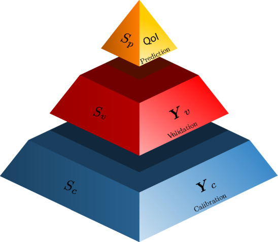
Bayesian prediction pyramid showing three levels; calibration, validation, and prediction. Model is calibrated using the data ${\mathit{Y}}_c$ obtained under the scenario $S_c$. Calibration scenarios are designed to test the sub-components of the model. Model is then validated using the data ${\mathit{Y}}_v$ obtained under scenario $S_v$. Validation scenarios are more complex as compared to calibration scenarios. Finally, the calibrated-validated model is employed to predict quantities of interest under the scenario $S_p$. Scenario $S_p$ represents the conditions under which obtaining the data is either expensive or very difficult [11, 23, 24]

Model calibration

In this step, the model parameters are tuned so that the statistics of the output of the model agrees with that of the data. We assume that the data for model calibration correspond to the calibration scenario $S_c$. Let ${\pi }_c(\mathit{\theta }|S_c)$ be the prior probability distribution of the model parameters, ${\pi }_c({\mathit{Y}}_c|\mathit{\theta },S_c)$ be the conditional probability of the data when the parameter is fixed to $\mathit{\theta }$ (the likelihood function), ${\pi }_c(\mathit{\theta }|{\mathit{Y}}_c,S_c)$ be the conditional probability of the parameter for a given data ${\mathit{Y}}_c$ (posterior), and ${\pi }_c({\mathit{Y}}_c|S_c)$ be the evidence. Bayes’ rule relates the prior, likelihood, and the posterior as follows:

$$\begin{array}{c}\hfill {\pi }_c(\mathit{\theta }|{\mathit{Y}}_c,S_c)=\frac{{\pi }_c({\mathit{Y}}_c|\mathit{\theta },S_c){\pi }_c(\mathit{\theta }|S_c)}{{\pi }_c({\mathit{Y}}_c|S_c)}.\end{array}$$ 14

The evidence is the marginalization of the numerator in (14) so that the posterior ${\pi }_c(\mathit{\theta }|{\mathit{Y}}_c,S_c)$ is integrated to 1 with respect to $\mathit{\theta }\in \mathrm{\Theta }$. It is given by

$$\begin{array}{c}\hfill {\pi }_c({\mathit{Y}}_c|S_c)={\int }_{\mathrm{\Theta }}{\pi }_c({\mathit{Y}}_c|\mathit{\theta },S_c){\pi }_c(\mathit{\theta }|S_c)d\mathit{\theta }.\end{array}$$ 15

We consider log-normal priors to ensure that the samples of parameters remain positive, see Sect. 4 for more details. Suppose we consider COVID-19 data at first $N_c$ days as the calibration data, i.e. ${\mathit{Y}}_c={(\mathit{Y}(t_i))}_{i=1}^{N_c}$. In the scenario $S_c$, we consider the total number of infected and deceased cases in whole of Texas as the data. The corresponding parameter-to-observable map is $\mathit{d}(\mathit{\theta },S_c;t)=(d_1,d_2)$ with

$$\begin{array}{cc}\hfill d_1(\mathit{\theta },S_c;t)& ={\int }_{\mathrm{\Omega }}\sum _{a\in \{i,r,d\}}{\varphi }_a(\mathit{x},t)d\mathit{x},\hfill \\ \hfill d_2(\mathit{\theta },S_c;t)& ={\int }_{\mathrm{\Omega }}{\varphi }_d(\mathit{x},t)d\mathit{x}.\hfill \end{array}$$ 16

The likelihood function is simply the product of likelihood function at each time $t_i$, $i=1,2,\dots ,N_c$,

$$\begin{array}{cc}\hfill {\pi }_c({\mathit{Y}}_c|\mathit{\theta },S_c)& =\prod _{i=1}^{N_c}L(\mathit{\theta },S_c;t_i)\hfill \\ \hfill & =\prod _{i=1}^{N_c}\prod _{j=1}^2\mathcal{N}(Y_{\mathit{cj}}(t_i)-d_j(\mathit{\theta },S_c;t_i),{\sigma }_j(t_i)),\hfill \end{array}$$ 17

where we substituted the form of $L(\mathit{\theta },S_c;t_i)$ from (13) and assumed that the noise in the infected cases and the deceased cases are not correlated and may depend on the time of the data.

As the prior and the likelihood functions are known, we can solve for the posterior ${\pi }_c(\mathit{\theta }|{\mathit{Y}}_c,S_c)$ using (14). (14) is solved numerically using the MCMC algorithm. These steps assimilate the data into the posterior ${\pi }_c(\mathit{\theta }|{\mathit{Y}}_c,S_c)$ which informs the sampling of parameters for an accurate model output.

Model validation

In this step, we validate the model by first tuning the parameters using the validation data obtained under the validation scenario $S_v$, and then computing the QoIs at validation times and comparing it with the data. Let ${\pi }_v(\mathit{\theta }|S_v)={\pi }_v(\mathit{\theta }|{\mathit{Y}}_c,S_c,S_v)$ be the prior for the validation step which is conditioned on the calibration data ${\mathit{Y}}_c$ and the scenario $S_c$. We take the calibration posterior ${\pi }_c(\mathit{\theta }|{\mathit{Y}}_c,S_c)$ as the validation prior, i.e. ${\pi }_v(\mathit{\theta }|{\mathit{Y}}_c,S_c,S_v)={\pi }_c(\mathit{\theta }|{\mathit{Y}}_c,S_c)$. Let ${\pi }_v({\mathit{Y}}_v|\mathit{\theta },{\mathit{Y}}_c,S_c,S_v)$ be the likelihood function, ${\pi }_v(\mathit{\theta }|{\mathit{Y}}_v,{\mathit{Y}}_c,S_c,S_v)$ be the validation posterior, and ${\pi }_v({\mathit{Y}}_v|{\mathit{Y}}_c,S_c,S_v)$ be the evidence.

Suppose the COVID-19 data at times $t_i$, for $i=N_c+1,N_c+2,\dots ,N_c+N_v$ defines the validation data, i.e. ${\mathit{Y}}_v={(\mathit{Y}(t_i))}_{i=N_c+1}^{N_v}$. Similar to calibration scenario, we let the total number of infected and deceased cases in Texas be the data in validation scenario $S_v$. P-to-o map $\mathit{d}(\mathit{\theta },S_v;t)$ is defined similarly to (16). The likelihood function is

$$\begin{array}{cc}& {\pi }_v({\mathit{Y}}_v|\mathit{\theta },{\mathit{Y}}_c,S_c,S_v)=\prod _{i=1}^{N_v}L(\mathit{\theta },S_v;t_{N_c+i})\hfill \\ \hfill & =\prod _{i=1}^{N_v}\prod _{j=1}^2\mathcal{N}(Y_{\mathit{vj}}(t_{N_c+i})-d_j(\mathit{\theta },S_v;t_{N_c+i}),{\sigma }_j(t_{N_c+i})),\hfill \end{array}$$ 18

As in the calibration step, we solve for the posterior ${\pi }_v(\mathit{\theta }|{\mathit{Y}}_v)$ using (14). For the validation of the model, we sample the parameter from the validation posterior, solve the forward problem $\mathcal{A}(\mathit{\theta },S_v;\mathit{u}(\mathit{\theta },S_v))=0$, and compute the QoI Q. If the difference of prediction (QoI in other words) and the data ${\mathit{Y}}_v$ is within the tolerance ${\gamma }_{\mathit{tol}}$, i.e.

$$\begin{array}{c}\hfill d(Q(\mathit{\theta },S_v;t_{N_c+N_v}),\mathit{Y}(t_{N_c+N_v}))\le {\gamma }_{\mathit{tol}},\end{array}$$ 19

then we declare the model as Not Invalid. Here, $d(·,·)$ is the metric that compares the two random fields, [24]. For the current model, we perform validation as follows: we consider the total infected and deceased cases in Texas as QoI and compute the standard deviation ${\sigma }_{\mathit{inf}}$ and ${\sigma }_{\mathit{dec}}$ of the normalized error in infected cases and deceased cases. With tolerance ${\gamma }_{\mathit{inf}}=0.08$ ($8\%$ error) and ${\gamma }_{\mathit{dec}}=0.04$ ($4\%$ error), we check if ${\sigma }_{\mathit{inf}}<{\gamma }_{\mathit{inf}}$ and ${\sigma }_{\mathit{dec}}<{\gamma }_{\mathit{dec}}$ to determine the validity of the model.

Model prediction

Suppose the model was found to be Not Invalid. We compute the total infected cases and total deceased cases, as well as the infected and deceased cases in each of 25 districts in Texas, at prediction days from $t=N_c+N_v+1$ to $t=T_p$. The QoIs so obtained are the random fields. Standard deviation of QoI indicates the uncertainty in the predictions.

Numerical approximation of forward problem and sensitivity analysis

In this section, we outline the numerical approximation of the forward model. The data, obtained from https://www.dshs.texas.gov/coronavirus/additionaldata/, consists of total population, total infected cases (sum of active infected, recovered, and deceased cases), deceased cases, and recovered cases for each of the 254 county in Texas. The number of recovered cases are not exact as noted in the source of the data. We process the county-wise data to obtain the data for each district and also total data in Texas. We let data in period June 1–June 20 as the calibration data and June 21–June 30 as the validation data. We obtain the map of Texas along with the district boundaries in shapefile format from http://gis-txdot.opendata.arcgis.com/datasets/texas-state-boundary. To triangulate the Texas region, we follow these steps:

1. Load the Texas map file in QGIS software. QGIS software is freely available.

2. Coarse grain the outer boundary segments using Simplify tool in QGIS. The original map has few very small length segments which may create problem in triangulation or result in very fine mesh.

3. Obtain the vertices using Extract Vertices tool in QGIS and save the vertices layer using save layer as option. Select As_XY in Graphical category while saving the file in a csv format.

4. Prepare a Gmsh input file using vertices file for triangulation.

In Fig. 3, we show the triangulation along with the total cases of infection and the total fatal cases in 25 districts at the beginning of model inference, i.e., 1st June 2020.

Fig. 3.

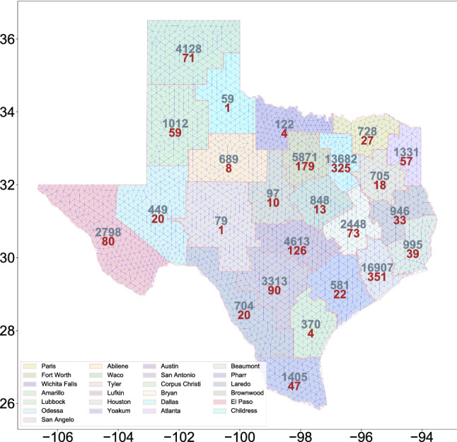
Map of the state of Texas state partitioned into 25 internal districts. The number of cases (grey) and deceased cases (red) in various districts as of $1^{\mathit{st}}$ June 2020 is also shown. In the background, the triangulation of the map is shown

Numerical discretization

Suppose $(·,·)$ denote the $L^2$ inner product over domain $\mathrm{\Omega }$. We assume homogeneous Neumann boundary condition for all densities. Let $V_a=H^1(\mathrm{\Omega })$ for $a\in \{s,e,i,r,d,n\}$ and $V_a^h$ be the finite dimensional approximation of $V_a$ by continuous piecewise linear interpolations over triangulation ${\mathcal{T}}^h$. Suppose ${\varphi }_{a_n}\in V_a^h$ denote the solution at time $t_n$. Given ${\{{\varphi }_{a_n}\}}_{a\in \{s,e,i,r,d\}}$, we seek ${\varphi }_{a_{n+1}}$ at time $t_{n+1}=t_n+\mathrm{\Delta }t$. Since the equations for ${\varphi }_a$ are nonlinearly coupled, we consider a fixed point iteration at each time step. Let ${\varphi }_a^k,{\varphi }_a^{k+1}\in V_a^h$ denote the current iteration and next iteration (unknown) approximation of ${\varphi }_{a_{n+1}}$ and let ${\tilde{\varphi }}_a\in V_a^h$ denote the test function. At iteration step k at time $t_n$, weak forms for susceptible, exposed, infected, and deceased density fields are as follows:

1. Susceptible

$$\begin{array}{cc}& ({\varphi }_s^{k+1},{\tilde{\varphi }}_s)+\mathrm{\Delta }t\left(\left(1,-,\frac{A}{{\varphi }_n^k}\right),{\beta }_i,{\varphi }_i^k,{\varphi }_s^{k+1},,,{\tilde{\varphi }}_s\right)\hfill \\ \hfill & +\mathrm{\Delta }t\left(\left(1,-,\frac{A}{{\varphi }_n^k}\right),{\beta }_e,{\varphi }_e^k,{\varphi }_s^{k+1},,,{\tilde{\varphi }}_s\right)\hfill \\ \hfill & +\mathrm{\Delta }t(\mu {\varphi }_n^k{\varphi }_s^{k+1},{\tilde{\varphi }}_s)+\mathrm{\Delta }t({\nu }_s{\varphi }_n^k\mathrm{\nabla }{\varphi }_s^{k+1},\mathrm{\nabla }{\tilde{\varphi }}_s)\hfill \\ \hfill & =({\varphi }_{s_n},{\tilde{\varphi }}_s)+\mathrm{\Delta }t(\alpha {\varphi }_n^k,{\tilde{\varphi }}_s).\hfill \end{array}$$ 20

2. Exposed

$$\begin{array}{cc}& ({\varphi }_e^{k+1},{\tilde{\varphi }}_e)+\mathrm{\Delta }t((\sigma +{\gamma }_e){\varphi }_e^{k+1},{\tilde{\varphi }}_e)\hfill \\ \hfill & +\mathrm{\Delta }t(\mu {\varphi }_n^k{\varphi }_e^{k+1},{\tilde{\varphi }}_e)+\mathrm{\Delta }t({\nu }_e{\varphi }_n^k\mathrm{\nabla }{\varphi }_e^{k+1},\mathrm{\nabla }{\tilde{\varphi }}_e)\hfill \\ \hfill & =({\varphi }_{e_n},{\tilde{\varphi }}_e)+\mathrm{\Delta }t\left(\left(1,-,\frac{A}{{\varphi }_n^k}\right),{\beta }_i,{\varphi }_s^{k+1},{\varphi }_i^k,,,{\tilde{\varphi }}_e\right)\hfill \\ \hfill & +\mathrm{\Delta }t\left(\left(1,-,\frac{A}{{\varphi }_n^k}\right),{\beta }_e,{\varphi }_s^{k+1},{\varphi }_e^k,,,{\tilde{\varphi }}_e\right).\hfill \end{array}$$ 21

3. Infected

$$\begin{array}{cc}& ({\varphi }_i^{k+1},{\tilde{\varphi }}_i)+\mathrm{\Delta }t(({\gamma }_d+{\gamma }_r){\varphi }_i^{k+1},{\tilde{\varphi }}_i)\hfill \\ \hfill & +\mathrm{\Delta }t(\mu {\varphi }_n^k{\varphi }_i^{k+1},{\tilde{\varphi }}_i)+\mathrm{\Delta }t({\nu }_i{\varphi }_n^k\mathrm{\nabla }{\varphi }_i^{k+1},\mathrm{\nabla }{\tilde{\varphi }}_i)\hfill \\ \hfill & =({\varphi }_{i_n},{\tilde{\varphi }}_i)+\mathrm{\Delta }t(\sigma {\varphi }_e^{k+1},{\tilde{\varphi }}_i).\hfill \end{array}$$ 22

4. Recovered

$$\begin{array}{cc}& ({\varphi }_r^{k+1},{\tilde{\varphi }}_r)+\mathrm{\Delta }t(\mu {\varphi }_n^k{\varphi }_r^{k+1},{\tilde{\varphi }}_r)+\mathrm{\Delta }t({\nu }_r{\varphi }_n^k\mathrm{\nabla }{\varphi }_r^{k+1},\mathrm{\nabla }{\tilde{\varphi }}_r)\hfill \\ \hfill & =({\varphi }_{r_n},{\tilde{\varphi }}_r)+\mathrm{\Delta }t({\gamma }_r{\varphi }_i^{k+1},{\tilde{\varphi }}_r)+\mathrm{\Delta }t({\gamma }_e{\varphi }_e^{k+1},{\tilde{\varphi }}_r).\hfill \end{array}$$ 23

5. Deceased

$$\begin{array}{c}\hfill ({\varphi }_d^{k+1},{\tilde{\varphi }}_d)=({\varphi }_{d_n},{\tilde{\varphi }}_d)+\mathrm{\Delta }t({\gamma }_d{\varphi }_i^{k+1},{\tilde{\varphi }}_d).\end{array}$$ 24

The fields ${\varphi }_a^{k+1}$ are solved in the same order as their weak forms are presented above. Note that in weak form for ${\varphi }_e$, we consider updated solution ${\varphi }_s^{k+1}$ instead of ${\varphi }_s^k$. Similar is true for other equations. Algorithm 1 provides the key steps required to solve the forward problem. The solver is implemented through FEniCS [1, 20]. The resulting linear systems in (20)–(24) are solved by the GMRES algorithm with the incomplete LU preconditioners.

Units

We let time be in the units of days and length in units of 100 km. Let ${\rho }_0=10000\text{people}/{(100\text{km})}^2$. The densities ${\varphi }_a$, $a\{s,e,i,r,d,n\}$, are in units of ${\rho }_0$. The parameters $\alpha ,{\gamma }_e,{\gamma }_r,{\gamma }_d,\sigma$ have unit of 1/day, parameters ${\beta }_i,{\beta }_e,\mu$ have unit of $1/({\rho }_0\text{day})$, A has unit of $1/{\rho }_0$, and ${\nu }_s,{\nu }_e,{\nu }_i,{\nu }_r$ have unit of ${(100\text{km})}^2/({\rho }_0\text{day})$.

Initial condition

We obtain the total population, total infected cases, deceased cases, recovered cases for each of the county from the data at $t=0$ (1st June 2020). To specify the initial population densities ${\varphi }_a$, $a\in s,e,i,r,d$, we proceed as follows: for ${\varphi }_a$, $a\in \{i,r,d,n\}$, we consider the following sum of 254 Gaussian functions centered at the centroid of counties:

$$\begin{array}{c}\hfill {\varphi }_a(\mathit{x},0)=\sum _{i=1}^{254}{A}_{i}exp\left[-,\frac{|\mathit{x}-{\mathit{x}}_{c,i}{|}^2}{2B_i^2}\right],\end{array}$$ 25

where $A_i$ is the amplitude of Gaussian, $B_i$ is the length scale controlling the decay, ${\mathit{x}}_{c,i}$ is the centroid of $i^{\text{th}}$ county. We take $B_i=\sqrt{\text{Area of county}i/(4\pi )}$ and choose amplitude such that the integration of individual Gaussian functions over the ${\mathbb{R}}^2$ is same as the number of cases (infected, recovered, deceased or total population depending on $a\in \{i,r,d\}$). This approach leads to $95.5\%$ of the number of cases in each county fall into a circle centered at its centroid with the radius approximated by square-root of its area. To determine the remaining two species, we first hypothesize that the exposed cases density is given by

$$\begin{array}{c}\hfill {\varphi }_e(\mathit{x},0)=R{\varphi }_i(\mathit{x},0).\end{array}$$ 26

Using the fact that ${\varphi }_n={\sum }_{a\in \{s,e,i,r,d\}}{\varphi }_a$, we determine ${\varphi }_s$. The parameter R in above is treated as the model parameter. We will see next the effect of parameter R on the total infected cases.

Sensitivity analysis

In this section, we perform a sensitivity analysis of quantities of interest on different parameters. We consider the total infected and total deceased cases as the QoI. We consider two settings. In the first setting, we fix ${\gamma }_e,{\gamma }_r,{\gamma }_d,\sigma$ according to Table 1 and let $\mathit{\theta }=(A,{\beta }_e,{\nu }_s,{\nu }_i,R)$ denote the model parameters. In the second setting, we include ${\gamma }_e,{\gamma }_r,{\gamma }_d,\sigma$ in the parameter list. In Table 1, we list the values of parameters reported in the previous study and their range considered in the sensitivity study.

Table 1.

Prior probability data: parameter values from previous studies [3, 30]. The values are converted to the appropriate units

Parameter	Value	Variance after $ln$	Range
${\gamma }_e$	1/6	0.25	[0.8/6, 1.25/6]
${\gamma }_r$	1/24	0.25	[0.75/24, 1.33/24]
${\gamma }_d$	1/160	0.25	[0.5/160, 2/160]
$\sigma$	1/7	0.25	[0.8/7, 1.25/7]
A	1000	0.4	[10, 1200]
${\beta }_e$	$3.3\times {10}^{-4}$	0.5	$[5\times {10}^{-5},{10}^{-3}]$
${\nu }_s$	$4.35\times {10}^{-6}$	0.5	$[{10}^{-7},{10}^{-4}]$
${\nu }_i$	${10}^{-8}$	1	$[5\times {10}^{-9},5\times {10}^{-6}]$
R	4.64	0.25	[0.2, 20]

We performed the convergence study to confirm that the model has been discretized correctly in space and time. The choice of mesh and time step were constrained by the fact that the PDEs have to be solved many times. The triangulation of map in this and the study in the next section consists of 2969 vertices and 5683 triangle elements. The mesh size is about 18.942 km. The final time is $T=20$ days and the size of time step is $\mathrm{\Delta }t=0.1$ day.

Table 3.

The mean, the variance in ln() of the parameter space, and the approximated mode for each parameters of interest derived from the validation posterior samples

Parameter	Mean	Variance after $ln$	Approximated mode
A	413	0.0569	379
${\beta }_{i,e}$	$3.78\times {10}^{-4}$	0.0592	$3.46\times {10}^{-4}$
${\nu }_{s,e,r}$	$3.94\times {10}^{-6}$	0.250	$2.70\times {10}^{-6}$
${\gamma }_r$	0.0658	0.0451	0.0614
${\gamma }_d$	$2.25\times {10}^{-3}$	0.0243	$2.07\times {10}^{-3}$
$\sigma$	0.0724	0.0353	0.0686
R	2.28	0.0618	2.08

Fig. 7.

The marginalized validation posterior densities (orange) and the marginalized validation prior densities (blue) for each parameters of interest

We employ open source library SALib and use the method of Morris [6, 21] for sensitivity calculation. We generate 1200 and 2000 samples of parameters for setting 1 and 2, and compute the total infected and deceased case for each parameter. In Fig. 4, we plot the ${\mu }^{\ast }$ (mean of the absolute value of the elementary effects), total infected and deceased QoIs at different parameter samples. From the plots, we note that while the variation in the infected QoI is very large indicating that the model can be calibrated. The variation in the deceased QoI is extremely small (below order 1) in setting 1 indicating that the model can not be calibrated for a given deceased data. The results of setting 2 show that the deceased QoI is most sensitive to parameters ${\gamma }_d,\sigma ,{\gamma }_r$ and the other parameters have almost no effect. For this reason the parameters ${\gamma }_d,\sigma ,{\gamma }_r$ are kept variable and learned from the data. Results also show the negligible effect of ${\gamma }_e,{\nu }_i$ on QoIs, and, therefore, their values are fixed from Table 1.

Fig. 4.

Sensitivity results for case when $\mathit{\theta }=(A,{\beta }_e,{\nu }_s,{\nu }_i,R)$ (on left) and $\mathit{\theta }=(A,{\beta }_e,{\nu }_s,{\nu }_i,{\gamma }_e,{\gamma }_r,{\gamma }_d,\sigma ,R)$ (on right). Top figures show parameters with higher ${\mu }^{\ast }$, the mean of the Morris elementary effects, for the two QoIs. Bottom figures show the QoI values at different samples. Note that the variation in total deceased cases is extremely small in setting 1

Inference results

We consider the total infected and deceased cases respectively in the period June 1–June 20 and June 21–June 30 as the calibration and validation data. We predict the number of infected and deceased cases for period July 1–September 1. We assume that ${\nu }_r={\nu }_e={\nu }_s$ and ${\beta }_i={\beta }_e$. Based on the sensitivity study in the preceding section, we fix values of ${\gamma }_e$ and ${\nu }_i$ from Table 1 and consider $\mathit{\theta }=(A,{\beta }_e,{\nu }_s,{\gamma }_r,{\gamma }_d,\sigma ,R)$. For the posterior sampling in the calibration and validation steps, we utilize the preconditioned Crank-Nicolson (pCN) algorithm implemented in the hIPPYlib library (version 3.0.0) [31, 32].

Calibration

We consider a log-normal prior with mode and variance for parameters given in Table 1. We note that for the parameter A, we consider a mode of 400 to ensure that A is not sampled often in a nonphysical regime. From the SEIRD model (1), the term $\left(1,-,\frac{A}{{\varphi }_n}\right){\beta }_i{\varphi }_s{\varphi }_i$ represents the portion of the susceptible population transitioning to exposed due to infected population. If A is such that $1-A/{\varphi }_n<0$ then the transmission direction is reversed which is nonphysical and undesired.

The pCN algorithm is employed for generating samples from the posterior distribution, which is ideal for the inference problems with high dimensional parameter spaces and Gaussian priors. We refer to the interested readers to [4, 5, 13] and the reference within for the theory associated with Markov chain Monte Carlo and the pCN algorithm. With multiple runs of the pCN algorithms with different step size factors $\beta$, we choose $\beta =0.3$ to maximize the efficiency of the posterior samples.

A set of $\sim 3500$ calibration posterior samples are obtained through running 4 independent chains, with an average acceptance rate of $20\%$. The results for the Bayesian calibration of the model parameters, including both a typical chain evolution of the model outputs and the marginalized calibration posterior densities are shown in Fig. 5. The model outputs of the calibration posterior samples match the data with reasonable precision. The marginalized calibration posterior densities indicate a higher recovery rate, a lower mortality rate, and a longer incubation period compared to our prior assumptions, with the approximated modes at $\sim 1/13.6{\text{day}}^{-1}$, $\sim 1/462{\text{day}}^{-1}$, and $\sim 1/12.2{\text{day}}^{-1}$ respectively. A summary of the mean, the variance, and the approximated mode is shown in Table 2. The model outputs for all the calibration posterior samples and the model output at the mean of the calibration posterior are plotted with the data in Fig. 6.

Fig. 10.

Prediction of the total infected cases and deceased cases in top five districts from June 1 to September 1 2020. Left side of the vertical line correspond to the calibration plus validation days. Right side of vertical line correspond to the prediction days

Fig. 5.

Results for the Bayesian calibration step. The left figure is a typical evolution of the model outputs at day 1, 10, and 20 along a MCMC chain that shows rapid mixing starting $\sim 200$ samples. The red line and the red shaded region corresponds to the data and the region within one standard deviation according to the likelihood model. The right figure shows the marginalized calibration posterior densities (orange) and the marginalized calibration prior densities (blue) for each parameters of interest

Table 2.

The mean, the variance in ln() of the parameter space, and the approximated mode for each parameters of interest derived from the calibration posterior samples

Parameter	Mean	Variance after $ln$	Approximated mode
A	707	0.116	594
${\beta }_{i,e}$	$3.17\times {10}^{-4}$	0.181	$2.42\times {10}^{-4}$
${\nu }_{s,e,r}$	$6.39\times {10}^{-6}$	0.254	$4.36\times {10}^{-6}$
${\gamma }_r$	0.0804	0.0575	0.0737
${\gamma }_d$	$2.23\times {10}^{-3}$	0.0214	$2.16\times {10}^{-3}$
$\sigma$	0.0866	0.0383	0.0817
R	2.82	0.0552	2.59

Fig. 6.

The model outputs at the calibration posterior samples. The red line and the red shaded region corresponds to the data and the region within one standard deviation according the likelihood model. The green line corresponds to the model output at the mean of the calibration posterior samples

Validation

We approximate the calibration posterior density by a log-normal density using its mean and variance and use it as the prior density for the validation step. We employ the pCN algorithm with the step size factor $\beta =0.3$ to sample from the validation posterior density. A set of $\sim 4500$ validation posterior samples are obtained through running 4 chains with an average acceptance rate of $30\%$. Using the validation posterior, we compute the total infected cases and deceased cases from $t=20$ to $t=30$ and compare with the data. The standard deviation of the normalized error in total infected and deceased cases are found to be $0.0863>{\gamma }_{\mathit{inf}}=0.08$ and $0.0068<{\gamma }_{\mathit{dec}}=0.04$. This implies that the model is Invalid for the infected QoI and Not Invalid for the deceased QoI. This conclusion is strengthened by the plots in Fig. 8 which shows that the model under predicts the infected cases whereas the model prediction of the deceased cases is very close to the data.

Fig. 8.

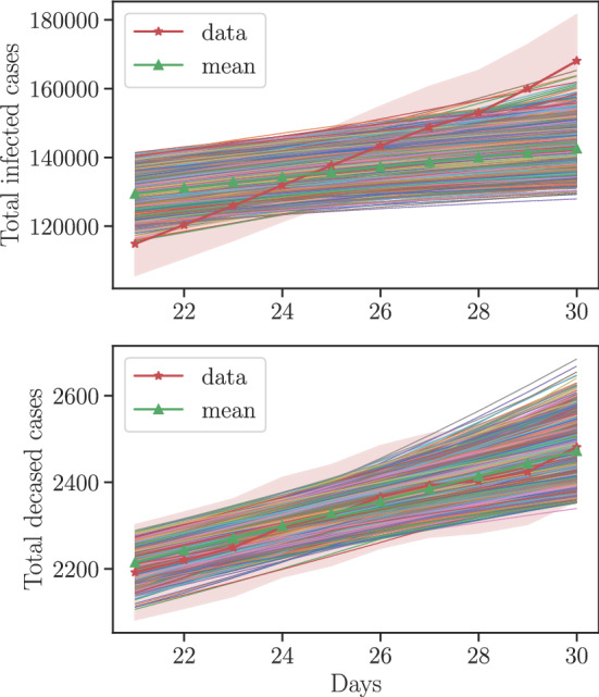
The model outputs at the validation posterior samples. The red line and the red shaded region corresponds to the data and the region within one standard deviation according the likelihood model. The green line corresponds to the model output at the mean of the validation posterior samples

Prediction

Using the validation posterior, we compute the total number of cases in 25 districts until September 1, 2020. The model predicts 7003 fatalities with $95\%$ CI 6802–7204 and 301658 total cases of COVID-19 infection with $95\%$ CI 290251–313064 in Texas by September 1, 2020. Uncertainty, in terms of the standard deviation of the quantity of interest, in the prediction for deceased and infected cases are 102 and 5786 respectively. Figure 9 shows the evolution of cases in Texas along with the confidence intervals. We select top five districts in terms of the total infected cases as of June 30, 2020 and plot the evolution of the cases in these five districts until September 1, 2020. Figure 11 shows the projection of the district QoIs by August 15 and September 1 on Texas map.

Fig. 9.

Prediction of the total infected cases and deceased cases in whole of Texas from July 1 to September 1 2020

Fig. 11.

Projection of total cases in 25 districts on August 15 (left) and September 1 (right). Red corresponds to the deceased cases and grey corresponds to the infected cases

Conclusion

Bayesian techniques have been employed to predict the COVID-19 spread in Texas. The model is found to be adequate to predict the deceased cases, however, falls short for the infected cases. By September 1, we predict to see about 7003 fatalities and 301658 infected cases. Uncertainties, in terms of the standard deviation of the QoI distribution, in deceased and infected cases are about 102 and 5786. Calculations show the SEIRD model employed in this work is not valid for the prediction of the infected cases. The cases of COVID-19 infection has been rising rapidly and it may be the case that the model is not adequate to account for the rapid increase in cases.

Several extensions of the model can be considered. For example, the model parameters can be allowed to vary in time and space; see [10, 17] where the parameters in ODE based SEIRD model are considered to be time dependent. Physical landscape or heterogeneities can be added to the model by considering non-homogenous and possibly anisotropic diffusion models [16]; higher infection diffusivity in densely populated counties, anisotropic diffusion to include the effects of highways/freeways. Another aspect believed to play a major role in the dynamics of COVID-19 spread is the asymptomatic/mildly symptomatic cases which are often not accounted in the data, see [7, 12, 19, 25, 29]. This work can be extended, similar to [26, 27], by subdividing the infected portion of the population into the asymptomatic and symptomatic groups to account for the effects of the unreported cases. OPAL provides a framework to rank models and select the best model for prediction. It can be applied to different variants of the SIR model such as SIS (susceptible-infected-susceptible), SEIR, SIRD, MSIR (M stands for immunity inherited from mother), SEIIR (II for infected but asymptomatic and infected but symptomatic), etc and find the best model for the prediction of the infected cases.

References

- 1.Alnæs MS, Blechta J, Hake J, Johansson A, Kehlet B, Logg A, Richardson C, Ring J, Rognes ME, Wells GN (2015) The fenics project version 1.5. Archive of Numerical Software 3:
- 2.Anastassopoulou C, Russo L, Tsakris A, Siettos C. Data-based analysis, modelling and forecasting of the covid-19 outbreak. PloS One. 2020;15:e0230405. doi: 10.1371/journal.pone.0230405. [DOI] [PMC free article] [PubMed] [Google Scholar]
- 3.Backer JA, Klinkenberg D, Wallinga J. Incubation period of 2019 novel coronavirus (2019-ncov) infections among travellers from Wuhan, China, 20–28 January 2020. Eurosurveillance. 2020;25:2000062. doi: 10.2807/1560-7917.ES.2020.25.5.2000062. [DOI] [PMC free article] [PubMed] [Google Scholar]
- 4.Beskos A, Pinski FJ, Sanz-Serna JM, Stuart AM. Hybrid Monte Carlo on Hilbert spaces. Stoch Process Appl. 2011;121:2201–2230. doi: 10.1016/j.spa.2011.06.003. [DOI] [Google Scholar]
- 5.Brooks S, Gelman A, Jones G, Meng X-L. Handbook of Markov Chain Monte Carlo. Boca Raton: CRC Press; 2011. [Google Scholar]
- 6.Campolongo F, Cariboni J, Saltelli A. An effective screening design for sensitivity analysis of large models. Environ Model Softw. 2007;22:1509–1518. doi: 10.1016/j.envsoft.2006.10.004. [DOI] [Google Scholar]
- 7.Chan JF-W, Yuan S, Kok K-H, To KK-W, Chu H, Yang J, Xing F, Liu J, Yip CC-Y, Poon RW-S, et al. A familial cluster of pneumonia associated with the 2019 novel coronavirus indicating person-to-person transmission: a study of a family cluster. The Lancet. 2020;395:514–523. doi: 10.1016/S0140-6736(20)30154-9. [DOI] [PMC free article] [PubMed] [Google Scholar]
- 8.Chen N, Zhou M, Dong X, Qu J, Gong F, Han Y, Qiu Y, Wang J, Liu Y, Wei Y, et al. Epidemiological and clinical characteristics of 99 cases of 2019 novel coronavirus pneumonia in Wuhan, China: a descriptive study. The Lancet. 2020;395:507–513. doi: 10.1016/S0140-6736(20)30211-7. [DOI] [PMC free article] [PubMed] [Google Scholar]
- 9.Dowd JB, Andriano L, Brazel DM, Rotondi V, Block P, Ding X, Liu Y, Mills MC. Demographic science aids in understanding the spread and fatality rates of covid-19. Proc Natl Acad Sci. 2020;117:9696–9698. doi: 10.1073/pnas.2004911117. [DOI] [PMC free article] [PubMed] [Google Scholar]
- 10.Dureau J, Kalogeropoulos K, Baguelin M. Capturing the time-varying drivers of an epidemic using stochastic dynamical systems. Biostatistics. 2013;14:541–555. doi: 10.1093/biostatistics/kxs052. [DOI] [PubMed] [Google Scholar]
- 11.Farrell K, Oden JT, Faghihi D. A bayesian framework for adaptive selection, calibration, and validation of coarse-grained models of atomistic systems. J Comput Phys. 2015;295:189–208. doi: 10.1016/j.jcp.2015.03.071. [DOI] [Google Scholar]
- 12.Gatto M, Bertuzzo E, Mari L, Miccoli S, Carraro L, Casagrandi R, Rinaldo A. Spread and dynamics of the covid-19 epidemic in Italy: effects of emergency containment measures. Proc Natl Acad Sci. 2020;117:10484–10491. doi: 10.1073/pnas.2004978117. [DOI] [PMC free article] [PubMed] [Google Scholar]
- 13.Hairer M, Stuart AM, Vollmer SJ. Spectral gaps for a metropolis-hastings algorithm in infinite dimensions. Ann Appl Probab. 2014;24:2455–2490. doi: 10.1214/13-AAP982. [DOI] [Google Scholar]
- 14.Hellewell J, Abbott S, Gimma A, Bosse NI, Jarvis CI, Russell TW, Munday JD, Kucharski AJ, Edmunds WJ, Sun F, Flasche S, Quilty BJ, Davies N, Liu Y, Clifford S, Klepac P, Jit M, Diamond C, Gibbs H, van Zandvoort K, Funk S, Eggo RM (2020) Feasibility of controlling COVID-19 outbreaks by isolation of cases and contacts. Lancet Glob Health 8(4):e488–e496. 10.1016/S2214-109X(20)30074-7 [DOI] [PMC free article] [PubMed]
- 15.Keeling MJ, Rohani P. Modeling infectious diseases in humans and animals. Princeton: Princeton University Press; 2011. [Google Scholar]
- 16.Keller JP, Gerardo-Giorda L, Veneziani A. Numerical simulation of a susceptible-exposed-infectious space-continuous model for the spread of rabies in raccoons across a realistic landscape. J Biol Dyn. 2013;7:31–46. doi: 10.1080/17513758.2012.742578. [DOI] [PMC free article] [PubMed] [Google Scholar]
- 17.Kucharski AJ, Russell TW, Diamond C, Liu Y, Edmunds J, Funk S, Eggo RM, Sun F, Jit M, Munday JD, Davies N, Gimma A, van Zandvoort K, Gibbs H, Hellewell J, Jarvis CI, Clifford S, Quilty BJ, Bosse NI, Abbott S, Klepac P, Flasche S (2020) Early dynamics of transmission and control of COVID-19: a mathematical modelling study. Lancet Infect Dis 20(5):553–558. 10.1016/S1473-3099(20)30144-4 [DOI] [PMC free article] [PubMed]
- 18.Li Q, Guan X, Wu P, Wang X, Zhou L, Tong Y, Ren R, Leung KSM, Lau EHY, Wong JY, Xing X, Xiang N, Wu Y, Li C, Chen Q, Li D, Liu T, Zhao J, Liu M, Tu W, Chen C, Jin L, Yang R, Wang Q, Zhou S, Wang R, Liu H, Luo Y, Liu Y, Shao G, Li H, Tao Z, Yang Y, Deng Z, Liu B, Ma Z, Zhang Y, Shi G, Lam TTY, Wu JT, Gao GF, Cowling BJ, Yang B, Leung GM, Feng Z (2020) Early transmission dynamics in Wuhan, China, of Novel Coronavirus–Infected Pneumonia. New Engl J Med 382(13):1199–1207. 10.1056/NEJMoa2001316 [DOI] [PMC free article] [PubMed]
- 19.Li R, Pei S, Chen B, Song Y, Zhang T, Yang W, Shaman J. Substantial undocumented infection facilitates the rapid dissemination of novel coronavirus (sars-cov-2) Science. 2020;368:489–493. doi: 10.1126/science.abb3221. [DOI] [PMC free article] [PubMed] [Google Scholar]
- 20.Logg A, Mardal K-A, Wells GN, et al. Automated solution of differential equations by the finite element method. Berlin: Springer; 2012. [Google Scholar]
- 21.Morris MD. Factorial sampling plans for preliminary computational experiments. Technometrics. 1991;33:161–174. doi: 10.1080/00401706.1991.10484804. [DOI] [Google Scholar]
- 22.Oden J (2017) Foundations of predictive computational sciences, ICES Reports
- 23.Oden JT. Adaptive multiscale predictive modelling. Acta Numer. 2018;27:353. doi: 10.1017/S096249291800003X. [DOI] [Google Scholar]
- 24.Oden JT, Babuška I, Faghihi D (2017) Predictive computational science: computer predictions in the presence of uncertainty. Encyclopedia of Computational Mechanics Second Edition 1–26
- 25.Pan X, Chen D, Xia Y, Wu X, Li T, Ou X, Zhou L, Liu J. Asymptomatic cases in a family cluster with sars-cov-2 infection. Lancet Infect Dis. 2020;20:410–411. doi: 10.1016/S1473-3099(20)30114-6. [DOI] [PMC free article] [PubMed] [Google Scholar]
- 26.Park SW, Cornforth DM, Dushoff J, Weitz, JS (2020) The time scale of asymptomatic transmission affects estimates of epidemic potential in the covid-19 outbreak, Epidemics, p 100392 [DOI] [PMC free article] [PubMed]
- 27.Peirlinck M, Linka K, Costabal FS, Bendavid E, Bhattacharya J, Ioannidis J, Kuhl E (2020) Visualizing the invisible: the effect of asymptomatic transmission on the outbreak dynamics of covid-19, medRxiv [DOI] [PMC free article] [PubMed]
- 28.Surveillances V. The epidemiological characteristics of an outbreak of 2019 novel coronavirus diseases (covid-19)–hina. China CDC Weekly. 2020;2(2020):113–122. [PMC free article] [PubMed] [Google Scholar]
- 29.Tang B, Xia F, Bragazzi NL, Wang X, He S, Sun X, Tang S, Xiao Y, Wu J (2020) Lessons drawn from china and south korea for managing covid-19 epidemic: insights from a comparative modeling study, medRxiv [DOI] [PMC free article] [PubMed]
- 30.Viguerie A, Lorenzo G, Auricchio F, Baroli D, Hughes TJR, Patton A, Reali A, Yankeelov TE, Veneziani A (2021) Simulating the spread of COVID-19 via a spatially-resolved susceptible–exposed–infected–recovered–deceased (SEIRD) model with heterogeneous diffusion. Appl Math Lett 111:106617. 10.1016/j.aml.2020.106617 [DOI] [PMC free article] [PubMed]
- 31.Villa U, Petra N, Ghattas O (2019) hIPPYlib: an extensible software framework for large-scale inverse problems governed by PDEs; Part I: deterministic inversion and linearized Bayesian inference. arxiv:1909.03948
- 32.Villa U, Petra N, Ghattas O (2018) hIPPYlib: an extensible software framework for large-scale deterministic and Bayesian inverse problems. J Open Source Softw 3(30):940. 10.21105/joss.00940