Improved Sea Ice Fraction Characterization for L-Band Observations by the Aquarius Radiometers

Abstract

Radiometers operating at L-band (1.4 GHz) are used to retrieve sea surface salinity over ice-free oceans and have been used recently to study the cryosphere. One hindrance of their use in the high latitudes is the preponderance of mixed scenes, where seawater and sea ice are both present in the sensor’s field of view (FOV). Accurately characterizing the scene is crucial for oceanographic and cryospheric applications. To that end, a sea ice fraction model, composed of passive microwave sea ice concentration retrievals and an instrument simulator that integrates radiative power coming from all around the antenna, is used. We investigate the model currently used operationally to derive the ice fraction affecting the Aquarius observations and show that it can be significantly improved. On the one hand, the current model tends to overestimate sea ice fraction in the marginal ice zone where observations are used for salinity retrievals. On the other hand, the current model underestimates ice fraction within the ice pack where observations are used to derive sea ice properties. For the northern hemisphere, we also find evidence of the sea ice type impact on L-band radiometric observations. We present a model to derive sea ice fractions that are in better agreement with Aquarius radiometric observations using the Advanced Microwave Scanning Radiometer 2 Bootstrap algorithm for sea ice concentration and using high-resolution integration over the sensor’s FOV.

I. Introduction

AQUARIUS instruments made passive and active microwave observations at L-band (frequency ~1.4 GHz and λ ~ 21 cm) from 2011 to 2015 with the primary purpose of retrieving sea surface salinity (SSS) [1], [2]. L-band has also been shown to be useful to study some elements of the cryosphere, such as sea ice (e.g. [3]), ice sheets (e.g. [4], [5]), snow properties [6], [7], and landscape freeze/thaw (e.g. [8]). In order to facilitate the use of Aquarius observations at the high latitudes, dedicated weekly polar gridded products were developed [4], [5].

Salinity observations in the high latitudes are a useful tool to monitor interactions between oceans and the cryosphere. Fresh water discharges from ice sheet melt result in large freshening signals that can impact large basins and global circulation [9]. However, the presence of sea ice makes the radiometric observations complex to interpret. An important parameter when using L-band observations in the high latitude oceans is the radiometer sea ice fraction (ICEF). ICEF determines the impact on the radiometric signal of the sea ice presence in the instrument field of view (FOV). Because brightness temperature of sea ice (>170 K) is much larger than that of seawater (<135 K for Aquarius incidence angles), even a small area of sea ice increases the radiometric signal, which can be misinterpreted as a change in salinity. SSS retrieved by Aquarius near Greenland exhibit seasonal cycles marked by freshening during the ice melt season. However, the largest observed freshening events occur each fall season when sea ice starts to form, leading to an ambiguity as to which signal is actually observed. ICEF is thus important when studying oceans (e.g., salinity variations resulting from freshwater inputs) and also when retrieving sea ice properties. Put simply, accurate ICEF is necessary to distinguish observations mostly influenced by seawater surface properties from those influenced by sea ice so that contaminated data can be identified and discarded. A step further is to use ICEF to correct observations for the contribution from the undesired source. This can be done either to remove water contribution when studying sea ice or to remove sea ice contribution when retrieving SSS. In both cases, having accurate estimates of ICEF is paramount to the optimal use of the observations in mixed scenes common in the polar regions.

ICEF currently provided in the Aquarius level 2 (L2) product (i.e., product version 4.0 and earlier) has been shown to exhibit inconsistencies when compared with Aquarius brightness temperatures (TB) (see Fig. 1 updated from [5, Fig. 11]). In particular, it is clear that ICEF is overestimated in many instances, as shown by the low values of observed TB when ICEF reaches large amounts (region I in Fig. 1). The large scatter in the relationship between TB and ICEF over the whole range of ICEF is also an indication of inaccurate ICEF, although it could result from complex sea ice physical conditions leading to a large variability in sea ice emissivity. One expects TB of sea ice to be variable because it is a mixture of materials (e.g., ice, brine, and air pockets) with varying amounts (e.g. [10]). In this paper, we investigate the origin of these inconsistencies by considering a different model for Aquarius ICEF and we reconcile Aquarius TB observations with ICEF estimations. The model presented in this paper will be used in the next release of the Aquarius products. Our study also provides useful guidance for the Soil Moisture Active Passive (SMAP) mission [11], which does not have an ice fraction model to date.

Fig. 1.

Aquarius brightness temperature (in kelvins) observed by the inner beam in vertical polarization as a function of the ice fraction provided in the Aquarius L2 product in the Ross Sea (with L2 data from cycle 85 to 105 between April 4, 2013 and August 29, 2013). The figure is an update of [5, Fig. 11] using V4.0 of the Aquarius L2 product released in June 2015. Also note that the data reported in the x- and y-axis are inverted compared with the original figure that reported ice fraction as a function of TBV.

Fig. 11.

Same as Fig. 10 for horizontal polarization instead of vertical polarization.

The ICEF is computed using an ancillary field of sea ice concentration integrated in the sensor FOV by accounting for the instruments properties (such as radiometer antenna gain pattern and pointing geometry). The ICEF currently in the Aquarius products uses a sea ice concentration analysis from the National Oceanic and Atmospheric Administration’s (NOAA’s) Marine Modeling and Analysis Branch (MMAB). In this paper, we show that using the operational sea ice concentration product from the Japanese Aerospace Exploration Agency (JAXA) derived from Advanced Microwave Scanning Radiometer 2 (AMSR2) measurements and the Bootstrap algorithm, and a high-resolution integration over the Aquarius radiometer FOV largely resolves the consistency issue between Aquarius TB and ICEF visible in Fig. 1. In Section II, we describe the Aquarius TB and sea ice concentration data used in our study. In Section III, the model to compute ICEF from the various sea ice concentration data sets is presented. In Section IV, we compare the ice concentration products and analyze their performance at explaining changes in TB observed by Aquarius. We also discuss the impact of different ice types. Section V summarizes our results and concludes on the benefits of the updated ICEF for Aquarius.

II. Data Description

A. Aquarius Product

We use TB observations from Aquarius L-band radiometers. Aquarius was launched in June 2011, started acquiring data in August 2011, and operated continuously until the mission’s ending due to spacecraft failure in June 2015. The spacecraft carrying Aquarius was in a polar (98° inclination) sun-synchronous orbit with 6 P.M. (6 A.M.) ascending (descending) node at the equator. There were three radiometers with beams pointing toward the right side of the spacecraft, toward the night side of the earth to limit contaminations by the Sun, which is a strong source at L-band [12]. The beams’ incidence angles ranged from 29.2° to 46.3° (Table I). The beams’ 3-dB footprints size ranged from 76 km × 94 km to 97 km × 156 km.

TABLE I.

Aquarius Radiometer Characteristics

Beam	Inner	Middle	Outer
Earth Incidence Angle	29.2°	38.4°	46.3°
3 dB footprint (along track (km) × across track (km))	76 × 94	84 × 120	97 × 156
Latitude Range	[79.0S – 85.0N]	[77.9S – 86.1N]	[76.5S – 87.4N]

We use the L2 data product of NASA’s official Aquarius Data Processing System (ADPS) available at https://podaac.jpl.nasa.gov/AquariusDataAccess. Data are reported along the ground tracks at 1.44-s temporal resolution, which is equivalent to an along track spatial sampling of ~10 km. We use the time and geolocation information (i.e., latitude and longitude of the beam’s footprint center), TB at the surface, and the radiometer ice fractions. The L2 radiometer ice fractions (L2ICEF hereafter) result from the integration in the instrument’s footprint of sea ice concentrations from NOAA MMAB (details are given in Section III).

The L2ICEF is used to generate the earth gridded products for SSS (i.e., level 3 products). In the ADPS product, ICEF between 0.001 and 0.01 raises the flag for moderate ice contamination, and ICEF between 0.01 and 0.5 raises the flag for severe contamination, which results in the exclusion of the retrieved SSS value from the level 3 product [13]. Overestimations of ICEF, such as apparent in region I in Fig. 1, can result in a decreased number of available SSS retrievals in the marginal ice zone. It can also increase the noise on existing SSS retrievals because level 3 products average all SSS available in a grid cell over various periods of time (daily, weekly, and monthly) in order to reduce the noise in the retrievals. Therefore, removing some, but not all, valid SSS retrievals from the average (because they were erroneously flagged as contaminated by ice) results in increased noise on level 3 SSS. Conversely, underestimated ICEF can increase the noise on level 3 SSS or create regional low SSS (freshwater) biases. In the polar gridded products [4], the average ICEF inside the grid cell is reported, but is not used to filter the SSS retrievals (this choice was left to the product user). For the polar gridded product, inaccurate L2ICEF reported in the grid cells will impact SSS filtering based on ice contamination threshold.

B. Satellite Observations and Algorithms for Sea Ice Concentration Retrievals

Three sea ice concentration products were considered in this paper, all are derived from passive microwave observations. The first product is from NOAA’s MMAB sea ice concentration analysis (http://polar.ncep.noaa.gov/seaice/Analyses.shtml). We use the field distributed in the global latitude–longitude grid [14] because it is also currently used operationally (product V4.0 and earlier) to compute the Aquarius L2ICEF. The global MMAB sea ice concentration field is produced daily on a 5-arcmin grid using the NASA Team algorithm version 1 [15] and version 2 [16], depending on the microwave sensor being used, combined with a procedure to remove false ice [17], [18]. For the period covered by Aquarius observations, the MMAB sea ice concentration field was obtained from several sensors. For a few weeks at the beginning of the Aquarius era (until October 3, 2011), the Advanced Microwave Scanning Radiometer—Earth Observing System (AMSR-E) was used. Then, the processing used the Special Sensor Microwave/Imager (SSM/I) on DMSP F-15 (October 7, 2011–present) and SSMIS on DMSP F-17 (June 19, 2012–present).

The other two sea ice concentration products used in this paper were obtained from the Bootstrap sea ice concentration Algorithm (BA) [19], [20]. BA is a state-of-the-art algorithm with a long history to generate sea ice concentrations. It makes use of three frequencies (18.7 GHz at vertical polarization, 23.8 GHz at vertical polarization, and 36.5 GHz at both vertical and horizontal polarizations). It is suited for generating long-term data sets needed for detailed studies of the variability and trends in the sea ice cover. There are several other sea ice concentration algorithms [21], but we considered the Bootstrap algorithm because of the availability of operationally retrieved sea ice concentration throughout the Aquarius mission lifetime (2011–2015) and the ongoing SMAP mission. Bootstrap has been applied to observations from SSMIS, AMSR-E, and AMSR2. The finest product’ spatial resolution (10 km) is obtained with AMSR2 (compared with AMSR-E and SSMIS). The AMSR2 BA (ABA) sea ice concentration product has been generated and distributed by JAXA’s Global Change Observation Mission portal (https://gcom-w1.jaxa.jp/) since May 2012 (AMSR-E products are available before that date). We use the level 3 daily sea ice concentrations that are provided for ascending and descending orbits in polar stereographic coordinates at 10-km spatial resolution. We average the ascending and descending orbits together as one daily field. When only one valid data was available, it was used as the daily value.

Finer spatial resolution of radiometric observations has enabled more accurate identification of the ice edge and improved characterization of the ice cover in the inner zones [10], which is an important aspect for our analysis. In order to distinguish the role of the method used to obtain sea ice concentration fields (e.g., MMAB versus Bootstrap) from the differences in spatial resolutions between AMSR2 and SSMIS (10 km versus 25 km), we also utilized Bootstrap sea ice concentration at 25-km resolution derived from SSMIS observations [22]. The SSMIS BA (SBA) sea ice concentration product is distributed by the U.S. National Snow and Ice Data Center (http://nsidc.org/data/nsidc-0079).

III. Model for Radiometer Sea Ice Fraction

ICEF is defined as the amount of sea ice present in the radiometer FOV weighted by the antenna gain pattern. It is a convenient quantity to assess the nature of Aquarius observations (e.g., ice, water, or mixture). For example, when studying the ocean, one needs observations that are mostly dependent on ocean features and impacted by ice as little as possible. The ICEF model is the combination of an ancillary data source for the sea ice concentration and an instrument simulator that integrates radiative power coming from all directions around the antenna [23], [24]. The instrument simulator is used to weight the contribution of the ice concentration at a given location on the earth depending on where it appears in the FOV.

An instrument like Aquarius, orbiting at 700-km altitude, has a FOV on the earth with a diameter of~ 5000 km. Most of the contributions to the observations are~coming from a narrower region of ~100 km in diameter, referred to as the 3-dB footprint, where the antenna gain is the largest. However, because sea ice has a much larger TB than seawater, it is important to account for contributions beyond the footprint and to perform the integration over the whole FOV. Even a fraction of ice outside the footprint can be important. For example, contamination by land (which exhibits a larger TB compared with ocean) has been shown to extend hundreds of kilometers away from the coast [23]. Fig. 2 shows an example of ice contamination in Aquarius observations over the ocean where little of the ice contamination comes from within the 3-dB footprint. The 3-dB footprint has a small fraction of its area covered with ice, with ice concentration being of 1% in a few 10-km grid cells (dark blue cells in Fig. 2). However, in this instance, the integrated ICEF is 1.1%. For Aquarius antenna, the 3-dB footprint represents only about half of the total integrated power. By comparisons, the integrated power inside 2.5 times the footprint is ~95%. For the case reported in Fig. 2, most of the ICEF relevant to interpret Aquarius observation comes from outside the instrument’s 3-dB footprint.

Fig. 2.

Map of sea ice concentration in the Ross Sea from the ABA product on April 4, 2013, with superimposed limits of Aquarius 3-dB footprint (red ellipsoid) and 2.5 times the footprint (red dashed line ellipsoid) for the inner beam. The first 5% of ice concentration has distinct colors at every 1% increment, and then concentration from 6% to 100% is a linear shading from dark gray to light gray. The inset at the bottom left shows the area around Antarctica reported in the main figure.

We compute the ICEF integrated over the earth FOV (⊕) as

$$\text{ICEF}={\int }_{\oplus }\text{SIC}\times G(\theta ,\phi )d\Omega /N$$ (1)

with G the total gain pattern (sum of copolarization and cross-polarization gains) for the beam under consideration (ICEF is computed separately for all three beams), SIC the sea ice concentration from the ancillary product interpolated at the antenna pattern sampling points, dΩ the solid angle element of integration, and N the normalizing factor given by

$$N={\int }_{\ominus }G(\theta ,\phi )d\Omega .$$ (2)

SIC is interpolated at the antenna pattern sampling points from the grid in which the ancillary data are provided (polar stereographic coordinates for ABA and SBA and global latitude–longitude sampling for MMAB). The antenna pattern is sampled in spherical coordinates around the antenna, where the antenna boresight is the main axis and the polarization plane (orthogonal to the boresight) is the reference plane. The polar angle off the boresight (θ) is sampled every 0.5° as well as the azimuth angle (φ) measured off the vertical polarization of the antenna [23], [24]. We use antenna patterns derived from numerical simulations of the antenna and spacecraft (the GRASP 2012 model discussed in [25]). Differences between antenna pattern models are typically small close to the boresight and should not impact ICEF significantly.

Because the simulator is computationally intensive, we have limited the spatial and temporal coverage of the computations used in this paper. In the northern hemisphere (NH), we limit computations to latitudes above 53.8N and to times between August 15, 2014 and October 14, 2014 (hereafter ‘NH summer’). The period of the year was selected to allow for the ice edge to be farther away from land surfaces to limit their impact on the measurements. To that end, we use only data that have a land fraction of 0.1% or less, as reported in the Aquarius L2 product. In the colder months, when the NH ice expands southward toward its maximum extent, the ice edge moves closer to land surfaces in North America, Europe, and Asia, which can compromise our analysis due to the uncertainty in land emissivity. For the southern hemisphere (SH), computations were conducted north of and in the Ross Sea, for times between April 4, 2013 and August 29, 2013 (hereafter ‘SH winter’) with the exclusion of a few days between May 10 and 15 due to missing swaths for the ABA product. These are the same conditions as for the data reported in Fig. 1, and the period is for an ice extent close to its maximum. Contrary to the NH, when the SH ice extends, it is surrounded by water. In order to allow for consistent comparisons between NH and SH results, we also report some results for NH winter and SH summer (see Table II), albeit with some caveats. For the NH winter, we had to relax the land contamination threshold from 0.1% to 1% in order to have enough data. For the SH summer, there are no data at very high ICEF because of the substantial decrease of sea ice in summer. We will focus our analysis on NH summer and SH winter cases.

TABLE II.

Start and End Dates for Case Studies of North Hemisphere (NH1 and NH2) and South Hemisphere (SH1 and SH2)

Case study	Start date	End date
NH1 winter	01-Feb-2014	31-Mar-2014
NH2 summer	15-Aug-2014	14-Oct-2014
SHI winter	04-Apr-2013	29-Aug-2013
SH2 summer	02-Jan-2014	30-Mar-2014

The computations were conducted using the MMAB, ABA, and SBA sea ice concentration products. A comparison between our computation using MMAB and the L2ICEF is reported in the Appendix. Our ICEF computations are consistent with L2ICEF, and TB dependence is the same as reported in Fig. 1. Our results exhibit slightly reduced scatter and fewer large outliers compared with L2ICEF, likely due to an enhanced numerical integration.

IV. Results

A. Comparison of Sea Ice Concentration Products

Fig. 3 reports maps of the MMAB and ABA sea ice concentration products used in this study and presented in Section II-B. In order to compare the fields from MMAB and ABA, the MMAB fields are regridded in the polar stereographic coordinates at 10-km spatial resolution. NH maps are for October 1, 2014, and SH maps are for August 1, 2013. In both hemispheres, the large-scale structures of the sea ice cover are very similar between both products, but important differences can be observed at small scales. This is the case in the marginal ice zone (where the ice concentration is lower), at the ice edge, and at some locations inside the ice pack. In general, MMAB ice concentration is lower and spatially more variable inside the ice pack than the ABA concentration, which shows more homogeneous and higher concentrations (dark red regions in the bottom row of Fig. 3). The ABA map also shows sharper transitions from ice to water at the ice edge (narrow transition from red to dark blue when the MMAB map shows regions of lighter blue). Maps of the differences in ice concentration between ABA and MMAB are reported for both hemispheres in Fig. 4 and show that MMAB is at least ~20% larger around the ice edge, for both the NH and SH, and it is at least ~20% lower over large areas within the ice pack.

Fig. 3.

Sea ice concentration maps (in %) from [(top left), (top right)] the MMAB product and [(bottom left), (bottom right)] ABA product, for [(top left), (bottom left)] the NH on October 1, 2014 and [(top right), (bottom right)] the SH on August 1, 2013.

Fig. 4.

Maps of the difference (in %) between ABA and MMAB sea ice concentrations presented in Fig. 3. (Left) October 1, 2014. (Right) August 1, 2013. The colorscale is saturated.

In order to compare ice concentration fields using AMSR2 observations and SSMIS observations, which have different spatial resolutions, the ABA fields are regridded at the SBA product resolution, namely, on a 25-km resolution polar stereographic grid. The regridding is done by averaging all AMSR2 10-km grid cell values falling inside a 25-km polar stereographic grid cell (drop-in-the-bucket approach). This 25-km regridded product will be referred to as ABA25 here-after. The difference between ABA25 and SBA is reported in Fig. 5 and shows a much better consistency between these ice concentration products compared with MMAB. The largest differences are concentrated in a very narrow area at the ice edge, likely due to the difference in resolution between the AMSR2 and SSMIS sensors (Table III) and the simple regridding process used for the ABA25 product (as indicated by the noisy nature of the differences, with dark blue and red cells next to each other). The consistency shown in Fig. 5 between two products using the Bootstrap algorithm with different sensors indicates that the large differences between ABA and MMAB (Fig. 4) are mostly due to the algorithm used to retrieve ice concentration and not the sensor used.

Fig. 5.

Maps of the difference (in %) between ABA25 and SBA sea ice concentrations for the same dates as in Fig. 4. (Left) October 1, 2014. (Right) August 1, 2013. The colorscale is saturated.

TABLE III.

Spatial Resolution of Various Sensors Used in Sea Ice Concentration Products

AMSR-E	AMSR2	SSMIS
18.7 GHz: 27 km × 16 km 23.8 GHz: 32 km × 18 km 36.5 GHz: 14 km × 8 km	18.7 GHz: 22 km × 14 km 23.8 GHz: 19 km × 11 km 36.5 GHz: 12 km × 7 km	19.35 GHz: 45 km × 74 km 22.235 GHz: 45 km × 74 km 37 GHz: 28 km × 45 km

We have produced difference maps such as those reported as examples in this section for every day during the periods under study (August 2014–October 2014 for NH and April 2013–August 2013 for SH) and found the results to be very consistent in time.

B. Comparison of Sea Ice Fractions From Different Sea Ice Concentration Products

In this section, we compare ice fractions that are ice concentrations integrated over Aquarius sensor’s gain patterns computed using the various sea ice concentration products compared in Section IV-A. ICEF is either from the Aquarius L2 product (L2ICEF) or calculated with the instrument simulator using the ABA and SBA ice concentration for the period and locations described in Section III. Fig. 6 reports a 2-D histogram of the distribution of the difference between the ABA ICEF and the L2ICEF for the NH and SH. For readability, the color represents the number of samples in logarithmic scale.

Fig. 6.

2-D histogram of ICEF difference between ABA and Aquarius L2ICEF as a function of L2ICEF using the inner beam in the (left) NH between August 15, 2014 and October 14, 2014 and (right) SH between April 4, 2013 and August 29, 2013. The color scale reports the number of samples in logarithmic scale.

In the NH [Fig. 6 (left)], the ICEF difference ABA–L2ICEF is mainly negative when L2ICEF is less than 0.3 and mostly positive above. This means that L2ICEF tends to be larger than ABA ICEF for low ICEF and lower in the ice pack, which is consistent with our comparisons of ice concentration (Fig. 4). In the SH [Fig. 6 (right)], the ICEF difference ABA–L2ICEF is mostly negative up to L2ICEF ~0.8, whereas it is mainly positive at high L2ICEF (>0.8). This means that the L2ICEF is larger over most of the ICEF range, except for the highest concentrations in the ice pack where it is smaller than ABA.

The high-density region at low L2ICEF is along the −1 slope line (bottom left boundary, between points 1 and 2 in Fig. 6). Along this line, the ICEF difference ABA L2ICEF is as large as the L2ICEF (but of opposite sign),−meaning that ABA does not indicate any sea ice and MMAB reports substantial sea ice concentration (up to ~0.3 in the NH and up to ~0.5 in the SH). The points in region I of Fig. 1, with large MMAB ICEF and low Aquarius TB characteristic of ice free water, contribute to the high-density region between points 1 and 2 in Fig. 6. Similar results as those obtained here in the Ross Sea would be obtained all around Antarctica. The high-density data in the region between points 3 and 4 (top right boundary) show regions with ABA retrieving fully covered icepack and MMAB retrieving a lower ice concentration.

Fig. 7 shows the ICEF difference SBA – L2ICEF. The results are very similar to those in Fig. 6 with ABA instead of SBA.

Fig. 7.

2-D histogram of ICEF difference between SBA and Aquarius L2ICEF as a function of L2ICEF using the inner beam in the (left) NH between August 15, 2014 and October 14, 2014 and (right) SH between April 4, 2013 and August 29, 2013. The color scale reports the number of samples in logarithmic scale.

An issue to consider for the results at the low end of ICEF is the difficulty to retrieve SIC at low concentrations. Assessments for SBA and NT2 algorithm report uncertainty estimates between 5% and 10% [26], [27], and analysis of the SBA algorithm suggests that the SSM/I data cannot provide accurate ice concentration below 8% [27]. In addition, Heygster et al. [28] report that at lower microwave frequencies such as L-band, thin ice has a lower TB than thicker ice resulting in lower effective ice concentration detected by the sensor. This could result in high biased SIC from sensors at higher frequencies compared with lower frequency TB. In order to estimate the impact of low end SIC uncertainty on Aquarius ICEF, we have computed ICEF for the SH case study using the ABA SIC and applying a 0.1 (10%) cutoff, namely, setting all SIC ≤ 0.1 to 0. We found that the impact on Aquarius ICEF is relatively small, usually less than 0.01 (1%). This order of magnitude reduction in ICEF compared with changes in SIC is due to the small area with SIC at or below 0.1 compared with the size of the Aquarius FOV (see an example in Fig. 2). This result illustrates the general behavior expected for errors in ICEF due to the coarser spatial resolution of Aquarius. Systematic errors in SIC will be mitigated in ICEF because only a fraction of Aquarius FOV is impacted, especially at the low end of ICEF for which most of the FOV is open water. Random errors will average out over the larger Aquarius FOV.

C. Comparison of Aquarius Ice Fractions and Observed TB

In this section, we report comparisons similar to Fig. 1 between TB observed by Aquarius and the ICEF computed from various ice concentration products. We quantify the variability, or scatter, of TB for a given ICEF using the sample quantile corresponding to a probability of 0.68 (Q68) as a metric instead of the standard deviation because of the possible impact of large outliers in the data on the standard deviation. For a normal distribution, 68% of the data are within ±1 standard deviation, and the 0.68 probability quantile and standard deviation are equivalent.

The results for the SH are reported in Figs. 8 and 9 for Aquarius TB observation in vertical and horizontal polarizations, respectively. Figs. 8 and 9 report Aquarius TB from the L2 as a function of (gray points) L2ICEF and (black points) ICEF calculated using the ABA ice concentration. The general dependence of TB to either L2ICEF or the newly calculated ABA ICEF is emphasized by computing the average TB in bins of 1% of ice fraction in red or blue, respectively. The ABA ICEF shows significantly improved consistency with Aquarius TB compared with L2ICEF. The TB relationship to ICEF is remarkably linear when using ABA over the whole range of ICEF. In contrast, TB versus L2ICEF exhibit large changes in slope, with close to a flat relationship for ICEF under 0.4, increased slope above 0.4 up to about ICEF of 0.9 when the relationship becomes flat again. This results in L2ICEF being generally much larger than ABA ICEF for ICEF up to 0.6 or TB up to 200 K. In particular, there does not seem to be a significant overestimation of ICEF in the low range with the ABA ICEF and the observed TB increases consistently with increasing ICEF ABA. This resolves the issue observed in region I in Fig. 1 and reported in [5]. The scatter with the ABA ICEF is also substantially reduced over most of the ICEF range with the Q68 being of 10 K or less, where the Q68 with L2ICEF can reach 20 K [Fig. 8 (right)]. While the Q68 is lower with L2ICEF in the low range of ICEF, it is due to TB being actually observed over ice-free ocean scenes that have a very low dynamic range in TB (of a few kelvins only). The L2ICEF thus appears largely overestimated leading to a larger overall error despite the small scatter in TB. Overall similar significant improvements when using ABA concentrations are obtained for the three Aquarius radiometers, and horizontal polarization.

Fig. 8.

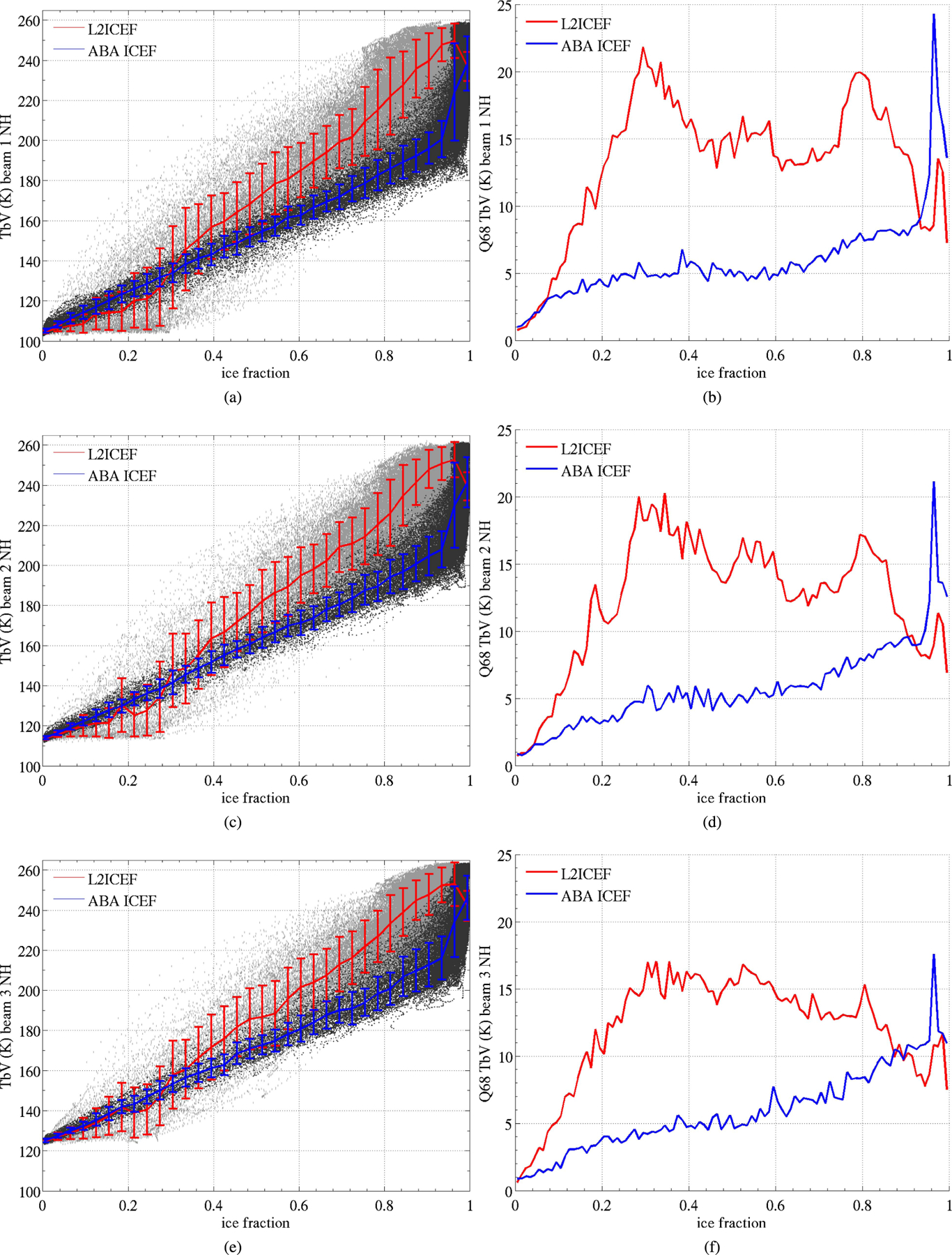
(Left) Brightness temperature in vertical polarization observed by Aquarius’ inner beam (top), middle beam (middle), and outer beam (bottom) as a function of sea ice fraction (ICEF) in the instrument FOV in the SH (Ross Sea) between April 4, 2013 and August 29, 2013. The ICEF is from the Aquarius L2 product (L2ICEF) (light gray and red curve) and our ICEF computed from ABA sea ice concentration product (dark gray and blue curve). In red and blue are (curves) the average TB and (error bars) the sample quantile corresponding to a 0.68 probability (Q68) of TB variation around its average computed inside 1% bins in ICEF. (Right) Q68 of the data reported on the left plots.

Fig. 9.

Same as Fig. 8 for horizontal polarization TB instead of vertical polarization.

The results in the NH (Figs. 10 and 11) also show improvements when using ice concentration from ABA. L2ICEF shows different regimes in the relationship between TB and ICEF, with smaller slopes in the ICEF range 0–0.2 and increased dependence of TB to ICEF for ICEF between 0.2 and 0.5. The relationship is largely more linear over the whole range of ICEF when using ABA, except where ICEF > 0.96, which shows a large uptick in TB. The scatter is also very significantly reduced with ABA, except at very high ICEF values. The Q68 is reduced to 5 K or less for ICEF of 0.2 or less, when L2ICEF exceeds 10 K at SIC of 0.2. Similar to the SH, but less pronounced, L2ICEF shows a cluster of points aligned with the x-axis, with fairly constant TB and large changes in L2ICEF, ranging from 0.0 to 0.3, due to the overestimations of ICEF in the MMAB model near the ice edge. The large spike in variance for ABA close to ICEF=1, exceeding L2ICEF and reaching 15 K, is due in large part to the sharp uptick in TB that is not resolved by the bin size used to compute the Q68. Estimating the error from Q68 inside the bins is reasonable if the underlying change in ICEF and resulting TB is small, which is true most of the time but not close to ICEF = 1 for ABA. We investigate a possible cause for the uptick at large ICEF in Section IV-D.

Fig. 10.

Same as Fig. 8 for the NH between August 15, 2014 and October 14, 2014.

Slopes of TB as a function of ICEF and Pearson’s correlation coefficient are reported in Tables IV and V. They are computed for the ABA ICEF only because L2ICEF is highly nonlinear, using data for ICEF between 0.1 and 0.8 to avoid open water and the uptick at high ICEF. For all cases, the Pearson correlation coefficient is high (>0.9). Slopes in the SH winter are ~30% larger than in the NH summer, in part due to the different seasons being assessed (see also Section IV-E). Slopes in winter are larger than in summer for both hemispheres, possibly due to the presence of open waters and melt ponds in the sea ice in summer.

TABLE IV.

Slopes (Columns 2–5) and Slope Ratios (Columns 6–9) of the Linear Regression of Aquarius TB as a Function of ABA ICEF in Kelvins per 0.01 Fraction, Computed for ICEF Between 0.1 and 0.8

Slope TB/ICEF (K/%)					Slope Ratio
Channel	NH winter	NH summer	SH winter	SH summer	NH winter/summer	SH winter/summer	winter SH/NH	summer SH/NH
V1	1.229	0.994	1.33	1.08	1.24	1.23	1.08	1.09
V2	1.258	1.004	1.297	1.042	1.25	1.24	1.03	1.04
V3	1.206	0.964	1.232	1.009	1.25	1.22	1.02	1.05
H1	1.287	1.054	1.421	1.164	1.22	1.22	1.10	1.10
H2	1.386	1.131	1.476	1.196	1.23	1.23	1.06	1.06
H3	1.442	1.174	1.53	1.277	1.23	1.20	1.06	1.09

TABLE V.

Pearson’s Correlation Coefficient for Aquarius TB and ABA ICEF Computed for ICEF Between 0.1 and 0.8

Channel	NH winter	NH summer	SH winter	SH summer
V1	0.951	0.962	0.967	0.962
V2	0.959	0.963	0.967	0.977
V3	0.972	0.956	0.975	0.977
H1	0.941	0.957	0.967	0.966
H2	0.944	0.956	0.969	0.974
H3	0.955	0.949	0.976	0.98

In order to investigate whether the higher spatial resolution of AMSR2 or the use of Bootstrap is the cause for the improved consistency between ICEF and Aquarius TB, we looked at the ICEF computed with the SBA ice concentrations that use the same algorithm as ABA but with satellite data at a coarser spatial resolution. The results are reported in Fig. 12. The improvement with SBA ICEF is similar to that of ABA ICEF, except that the Q68 is a bit larger (by up to 2 K for ICEF lower than 0.8), likely due to the coarser spatial resolution of SBA.

Fig. 12.

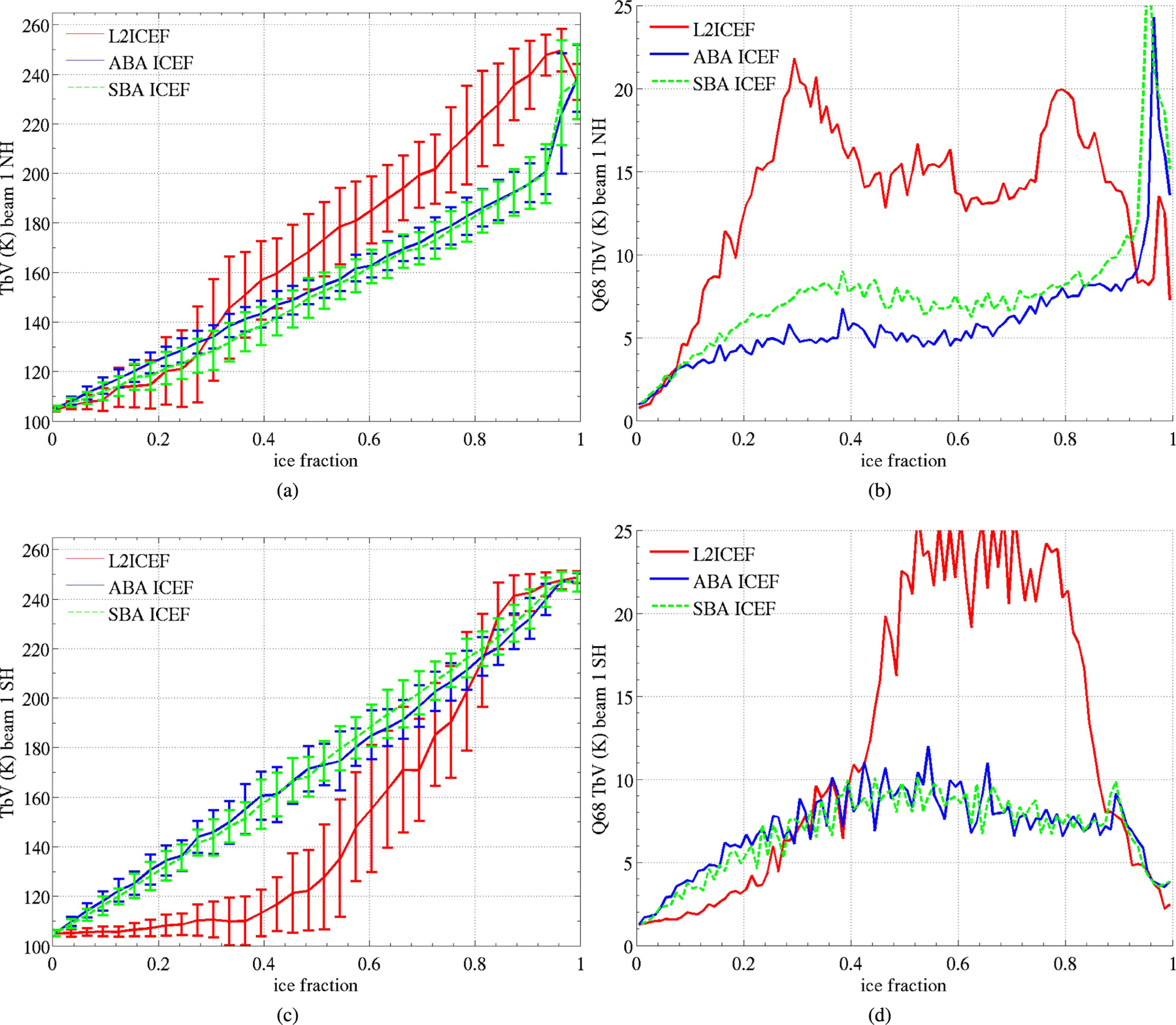
(Left) Aquarius TB for the inner beam and in vertical polarization as a function of ICEF from Aquarius L2 product (L2ICEF) (red curve), and our computation using the SBA (green curve) and ABA (blue curve) sea ice concentration products. (Right) Q68 of data on the left plots. The blue curves for the ABA ICEF are from Figs. 8 and 10 and are reported here for reference. The top row is for the NH between August 15, 2014 and October 14, 2014, corresponding to Fig. 10(a) and (b), and the bottom row is for the SH between April 4, 2013 and August 29, 2013, corresponding to Fig. 8(a) and (b). Also see caption of Fig. 8 for more details.

In order to illustrate the improvement of the new characterization of sea ice and its consistency with observed TB when approaching the ice edge, two examples of along track data are reported in Fig. 13 during a satellite fly over from ocean to the sea ice pack [Fig. 13 (left)] and from the sea ice pack to ocean [Fig. 13 (right)]. Different ICEFs are reported alongside observed TB. The ABA ICEF follows the changes in TB much closer than L2ICEF over most of the ICEF range. To quantify the shift along track of the ICEF curves, we use an example threshold of 1% ICEF. The shift between the location of the threshold between ABA and L2ICEF is of 37 km (left) and 75 km (right), with ABA threshold being reached closer to the ice pack, leading to less TB observation being flagged as contaminated by sea ice. For a threshold of 10% ICEF, the shift is 54 km (right). Therefore, using the ABA ICEF will allow for the use of observations closer to the ice edge by 50–80 km. Such observations are discarded when using L2ICEF due to the overestimated presence of ice. For the largest ICEF, in the ice pack, the ABA ICEF will allow for more accurate correction of the fraction of water in the FOV in order to study the sea ice properties.

Fig. 13.

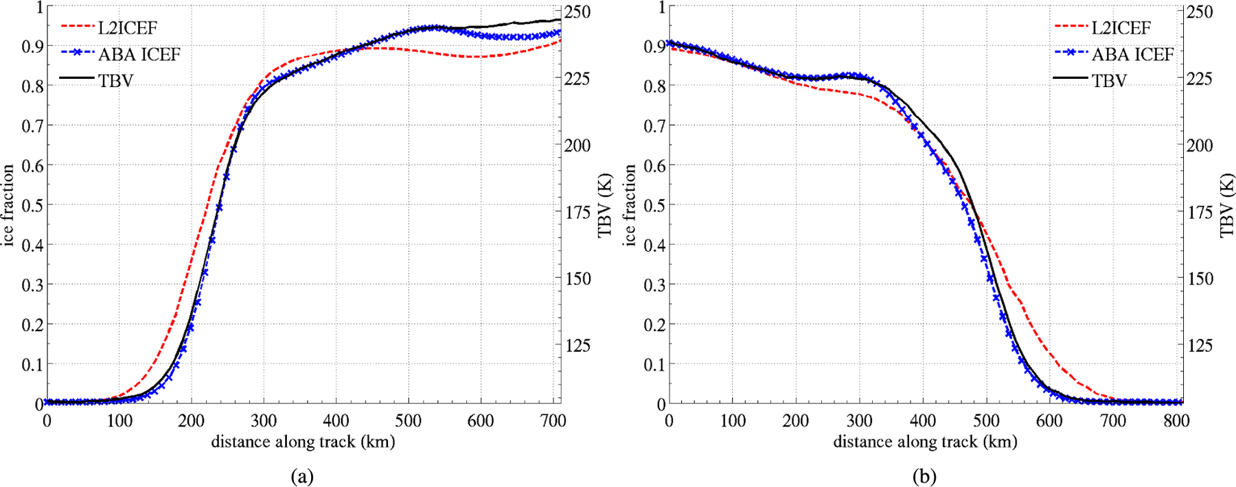
Two examples of difference in ICEF and observed TB along track during a fly over from ocean to sea ice pack (left) and from sea ice pack to ocean (right). TB observed by Aquarius (black curve) along satellite track and associated sea ice fraction from the Aquarius L2 product (L2ICEF) (red curve) and our computation using the ABA sea ice concentration product (blue curve). The tracks are part of the tracks reported in the inset of Fig. 1 and start on April 6, 2013 at 13h55m13s (left) and April 8, 2013 at 06h50m36s (right).

D. Impact of Multiyear Ice on TB in the NH

While the results in Figs. 10 and 11 show a linear TB relationship to ABA ICEF for ICEF in the range 0.00–0.96, they also show an uptick in the TB for ICEF approaching 1. This uptick occurs clearly in the NH only. In this section, we investigate a possible effect of different sea ice types on these results. To distinguish between multiyear (MY) and first-year (FY) ice, we use the product from the European Organization for the Exploitation of Meteorological Satellites (EUMET-SAT) Ocean and Sea Ice Satellite Application Facility (OSI SAF) (ftp://osisaf.met.no/archive/ice/type/) that provides daily maps with primarily two sea ice classes (FY and MY ice), a third class named ambiguous existing essentially during the melt season [29]. We focus on the NH as the uptick in TB was not observed for the SH. It should also be noted that MY ice is much less frequent in the Antarctic due to ocean currents and atmospheric circulation causing most of the ice to melt in the summer as it moves into warmer waters. We use data between September 15, 2014 and October 14, 2014 (after the melt season ended) because ice type maps before that period show a large amount of data classified as ambiguous. The OSI SAF also warns that during Arctic summer season, the ice type product is dubious because melting of the ice surface obscures the ice type signals. We also exclude data around October 1, 2014 due to a swath of missing data in the ice type map. We apply the ice type maps at 10-km resolution as a mask to the ABA ice concentrations in order to compute two different ICEFs for FY and MY ice. During the selected period, the ambiguous data in the ice type maps are limited to the narrow edge that parts the MY and FY regions. We apply a factor 0.5 to this region, namely, we count these grid cells as being half MY ice and half FY ice. The small hole without satellite observations around the north pole is assumed to be covered with MY ice (this has no significant effect on our results).

Fig. 14 reports the ICEF for MY ice as a function of the total ICEF (from ABA) and shows that MY ice is usually significant only where the largest ICEF values are observed, confirming the possibility of two regimes of TB being observed for low–moderate ICEF and for the largest ICEF (>0.96). The impact of the ice type is further confirmed in Fig. 15, which clearly shows that the highest TBs are associated with the largest fractions of MY ice. To assess further the differences in FY and MY ice, we compute the histogram of Aquarius TB for MY and FY ice separately only when the total ABA ICEF is larger than 0.96 (Fig. 16). The distribution widths are large, likely related to the variety of sea ice geophysical properties affecting the microwave radiation (e.g., temperature, brine content, and thickness) [30], [31]. In addition, a simple ice type classification into FY and MY is an idealization, and the FOV of the sensor is likely to contain a mixture of various ice types. However, the MY ice is clearly associated with larger TB on average than FY ice. The difference in average TB ranges from 20 K (V-pol, outer beam) to 40 K (H-pol, outer beam) with the MY ice having larger TB at all polarizations and incidence angles than FY ice (see Table VI).

Fig. 14.

Relationship between MY ice fraction and total ice fraction for Aquarius inner beam computed in the NH between September 15, 2014 and October 14, 2014. The y-axis reports the MY ABA ICEF, and the x-axis reports the total ABA ICEF. MY ice becomes significant only for the largest ICEF in Aquarius FOV.

Fig. 15.

Brightness temperature observed in the NH between September 15, 2014 and October 14, 2014 by Aquarius’ inner beam (top), middle beam (middle), and outer beam (bottom) in vertical (left) and horizontal (right) polarizations, as a function of sea ice fraction (ICEF) computed from the ABA product. The colors report the ICEF for MY ice only.

Fig. 16.

Histograms of TB observed in the NH between September 15, 2014 and October 14, 2014 by Aquarius’ inner beam (top), middle beam (middle), and outer beam (bottom) at vertical (left) and horizontal (right) polarizations. Histograms are computed for total ICEF > 0.96 and are separated by FY ice (blue bars) and MY ice (red bars).

TABLE VI.

Brightness Temperature for FY and MY Ice Computed as the Mode of the Distribution of Aquarius Brightness Temperatures in Kelvin. The Median Is Reported In Parentheses and Is Usually a Couple of Kelvins Smaller Than the Mode

	V-po1 (FY)	V-pol (MY)	H-po1 (FY)	H-pol (MY)
B1 @ 29°	232 (231)	255 (252)	220 (218)	249 (244)
B2 @ 38°	235 (236)	258 (257)	214 (214)	248 (245)
B3 @ 46°	241 (239)	262 (260)	208 (208)	247 (245)

In order to assess whether our results are consistent with other L-band instruments, we also looked at the data from the SMAP mission [11], which uses an L-band radiometer similar to Aquarius albeit with a better spatial resolution of 40 km. We do not integrate the ice concentration on the SMAP radiometer FOV as we did with Aquarius. We collocate the center of SMAP footprints with the ice type maps from OSI SAF and perform a nearest neighbor interpolation to assign the observed SMAP TB to FY or MY ice. The time period chosen is from November 1, 2015 to November 30, 2015. It is not possible to use the same time period as for the Aquarius study because SMAP started acquiring data only on March 30, 2015. The earlier part of the season (September–October 2015) is not used because it is characterized by ambiguous ice type values or has almost no FY ice.

Fig. 17 shows a comparison of the spatial distributions of SMAP TB in vertical polarization and the MY ice at the beginning and end of November 2015 [Fig. 17 (left) and (center)] and histograms of SMAP TB for FY and MY ice [Fig. 17 (right)]. The color scale in the maps is split at a TB of 255 K based on the separation of the histograms for FY and MY ice. The gray tones (above 255 K) report TBs mostly associated with MY ice, while the blue–red scale is mostly associated with FY ice. The green contour is the boundary between FY and MY ice from the OSI SAF product. The boundaries of the gray shapes and the green lines denote a good qualitative agreement between SMAP largest TB and the MY ice spatial distributions, confirming that L-band observations are sensitive to ice type. The temporal evolution [Fig. 17 (left) compared with (center)] also shows good agreement. For example, at the end of November, the MY ice expands to lower latitude along the northeast coast of Greenland and the MY ice recesses to higher latitudes north of Franz Joseph Land (on the right of the north pole in Fig. 17). There are locations with notable discrepancy between SMAP TB and ice type, for example, the large SMAP TB extends to lower latitudes toward the Laptev and East Siberian Seas (above the north pole in Fig. 17) than the MY ice from the OSI SAF product. For the TB histograms [Fig. 17 (right)], we use only data where ice concentration (as given by the product from OSI SAF) is above 96%. The histograms show results similar to those obtained with Aquarius. TBs exhibit a bimodal distribution that can be separated in two distributions depending on the ice type, with MY ice having larger mean TB than FY ice. The separation is not as clear as with Aquarius, and this could be due to several reasons. First, we do not perform the integration of ice types on SMAP FOV for this simple analysis aimed at confirming the results obtained with Aquarius. Therefore, we include cases of mixed FY and MY in both distributions. Also, the peak of the distribution of FY ice is broadened due to a temporal evolution of TB for FY ice. At the beginning of November, the FY ice TB histogram peaks at around 240 K. Later in the month, the peak is around 250 K, remaining lower than TB for MY ice that peaks around 259 K during the whole period.

Fig. 17.

SMAP TB distribution compared with FY and MY ice distribution. Maps of SMAP TB in vertical polarization in the NH are for November 6, 2015 (left) and November 28, 2015 (center), with the green contour line reporting the boundaries between the FY and MY ice derived from the OSI SAF product. Right: histogram of SMAP TB for FY ice (blue) and MY ice (red) for the whole month of November 2015.

Observations from both Aquarius and SMAP suggest an impact of the type of ice on L-band TB in agreement with experimental permittivity values obtained at 1 GHz [30]. MY ice contains less brine and more air pockets than FY ice because of the physical processes that occur during the summer melt. It is still to be determined how much various factors contribute to the larger TB of MY ice at L-band and possible factors are different composition and dielectric properties, different thicknesses, which is potentially more important at L-band due to the increased penetration compared with higher frequencies, and different locations for both types of ice leading to different average snow accumulations or melt amounts. Further studies are needed to assess these factors.

E. Seasonal Variations

The results in the previous sections have been reported for the NH summer and SH winter case study. Here we provide a short discussion of seasonal dependence of the relationship between Aquarius TB and ICEF. Computations have been conducted for the NH winter and SH summer, and comparisons between seasons and hemispheres are reported in Fig. 18 and Table IV.

Fig. 18.

Brightness temperature observed by Aquarius’ inner beam as a function of sea ice fraction (ICEF) in winter (left) and summer (right) in the NH (top) and SH (bottom) in vertical polarization. (Top left) NH winter (February 01, 2014-March 31, 2014). (Top right) NH summer (August 15, 2014–October 14, 2014). (Bottom left) SH winter (April 04, 2013–August 29, 2013). (Bottom right) SH summer (January 02, 2014–March 30, 2014).

Our main results are unchanged by the change of season. The ABA ICEF is in better agreement with Aquarius TB than L2ICEF for both seasons. The relationship between TB and ICEF is more linear, and there is less scatter with ABA ICEF than with L2ICEF. For both seasons, L2ICEF exhibits important departure from a linear relationship at ICEF less than 0.4, particularly in the SH, because of the overestimated SIC in the ancillary product. The relationship between TB and L2ICEF is better (more linear and with slopes closer to ABA) in the warmer seasons than in the colder seasons, particularly in the SH case study.

The main differences between seasons are a change in the slope of TB as a function of ICEF and a reduction in the TB uptick at high ICEF in the NH in winter (compared with summer). For a given hemisphere, the slopes’ TBs versus ICEFs (see Table IV) are higher in winter than in summer by 20%–25%. For a given season, slopes in the SH are higher than in the NH by 10% or less. Therefore, considering similar seasons brings slopes for both hemispheres closer to each other. However, slopes are still slightly higher in the SH. The uptick at high ICEF is less marked in the winter data for the NH than in summer, but it is still more pronounced than for the SH. The lower slopes in summer could be due to the impact of open water and melt pond. Lower frequency channels of AMSR-E have a smaller TB when the fractions of open water and melt water increase [32], and a similar effect is likely occurring at L-band.

V. Conclusion

Accounting accurately for the amount of sea ice present in the instrument FOV is crucial to the use of L-band radiometric data to study high latitudes, whether it is to study the oceans or the sea ice properties. We show that the sea ice fraction provided in the Aquarius product up to version 4.0 exhibits inconsistencies with the observed brightness temperatures. We compute a new sea ice fraction using a different sea ice concentration product derived from AMSR2 radiometric measurements and a simulator for the Aquarius instrument. We find a significantly improved relationship between TB observed by Aquarius and our new sea ice fraction. The occurrence of overestimated ice fractions is reduced, which leads to more data being available to retrieve SSS in cold waters. We also find an effect of the type of ice on radiometric observations, with the multiyear ice having on average higher L-band brightness temperatures than first year ice. In addition, the scatter in the relationship between radiometric observations and ice fraction is significantly reduced, which will facilitate the development of a correction for the impact of ice fraction on brightness temperature and the retrieval of SSS closer to the sea ice edge. Similarly, retrievals of sea ice properties (e.g., sea ice thickness) using L-band data will be enhanced by the improved sea ice fraction. We also find similar improvements from using sea ice concentrations derived from SSMIS measurements (instead of AMSR2) and the Bootstrap algorithm, despite the lower spatial resolution, with only a small increase in random error at some locations of the NH. This is important because the few times no AMSR2 data are available along some swaths, the algorithm will be able to use SSMIS-derived ice concentration as a backup with only little degradation in performances. Our results are also important for the recently launched SMAP mission [11], which is very similar to Aquarius, but with a finer spatial resolution that can make it more suitable for some studies at the high latitudes that often have a mixture of ice and water. The improved characterization of sea ice fraction presented in this paper will be implemented in the research product for polar regions (i.e., Aquarius weekly polar products distributed at https://nsidc.org/data/aquarius/) and in a future version of the official Aquarius product.

Biographies

Emmanuel P. Dinnat (M’12–SM’16) received the M.S. degree in instrumental methods in astrophysics and spatial applications in 1999 and the Ph.D. degree in computer science, telecommunications, and electronics from University Pierre and Marie Curie, Paris, France, in 2003.

He is currently a Research Scientist with the Center of Excellence in Earth Systems Modeling and Observations, Chapman University, Orange, CA, USA, and the Cryospheric Sciences Laboratory, NASA Goddard Space Flight Center, Greenbelt, MD, USA. His current research interests include active and passive microwave remote sensing, sea surface salinity, scattering from rough surfaces, atmospheric radiative transfer, and numerical simulation. He is involved in the calibration/validation and retrieval algorithms for the Soil Moisture and Ocean Salinity (SMOS), Aquarius/SAC-D and Soil Moisture Active Passive (SMAP) missions. His latest research focuses on high-latitude oceanography and the interactions between the cryosphere and oceans.

Ludovic Brucker (M’14) received the M.S. degree in physics from Blaise Pascal University, Clermont-Ferrand, France, in 2006, and the Ph.D. degree from the Laboratoire de Glaciologie et Geophysique de l’Environnement, Center National de la Recherche Scientifique, Grenoble Alpes University, Grenoble, France, in 2009.

He is currently with the NASA Goddard Space Flight Center, Greenbelt, MD, USA. His work contributes to the comprehension of the relationships between passive microwave air- and spaceborne observations and snow/ice physical properties using modeling approaches to provide climate-related variables to the community for the satellite era. He is involved in developing algorithms and state-of-the-art multilayer snow evolution and emission models. He has also participated in polar deployments in Antarctica, Greenland, and northern Canada. His current research interests include the investigation of climate evolution in the polar regions by interpreting space-borne microwave observations of snow-covered surfaces (sea ice, ice sheet, and terrestrial snowpacks).

Appendix. Impact of Numerical Integration on Ice Fraction

In order to assess the impact of the numerical integration on the computation of L2ICEF, we recomputed ICEF using our Aquarius numerical simulator and the same ancillary field as used currently in the L2 product (version 4.0 and earlier). We use two versions of the MMAB global sea ice concentration maps that are redistributed by Aquarius ADPS as part of the processing ancillary data (http://oceandata.sci.gsfc.nasa.gov/Ancillary/Meterological/). One data set is at the resolution of 1/12° (5 arcmin) in latitude and longitude, and the other has been smoothed at 0.5° (30 arcmin) resolution in latitude and longitude.

Fig. 19 shows an example of scatterplot of TB as a function L2ICEF and the ICEF computed using our model and the MMAB ancillary fields at the lower resolution of 0.5°. Our results are very similar to L2ICEF, and the differences between L2ICEF and our ICEF in Fig. 19 are much smaller than those reported in Section IV-C using a different ancillary field for the ice concentration. First, the shape of the relationship between TB and ICEF is largely conserved [Fig. 19 (left)], with a strong nonlinearity and significant scatter. In particular, there are still numerous instances of overestimations of ICEF (see region I in Fig. 1). Some differences between our results and L2ICEF can be observed with the large outliers, which are reduced with our computation. In general, our results show slightly less scatter, particularly for ICEF between 0.45 and 0.85, with a reduction in Q68 of a few kelvins [Fig. 19 (right)]. Still, the scatter is very significant and Q68 exceeds 10 K over a large range of ICEF.

Fig. 19.

(Left) Aquarius TB in the SH between April 4, 2013 and August 29, 2013 for the inner beam and in vertical polarization as a function of ICEF from Aquarius L2 product (L2ICEF) (light gray and red curves) and our computation using the MMAB sea ice concentration product (dark gray and green curves) at 30-arcmin (0.5°) spatial resolution. (Right) Q68 of data reported on the left plots. Also see the caption of Fig. 8 for more details.

Our results with the high-resolution MMAB do not show valuable improvements in the relationship between TB and ICEF [Fig. 20 (left)]. Most of the issues are still present, with a strong nonlinear dependence of TB to ICEF and a significant scatter in the relationship [Fig. 20 (right)].

Fig. 20.

Same as Fig. 19 using MMAB at 5-arcmin spatial resolutions instead of 30 arcmin for our computation.

References

- [1].Lagerloef G et al. , “The Aquarius/SAC-D mission: Designed to meet the salinity remote-sensing challenge,” Oceanogr. Mag, vol. 21, no. 1, pp. 68–81, March 2008. [Google Scholar]
- [2].Le Vine DM et al. , “Status of Aquarius/SAC-D and Aquarius salinity retrievals,” IEEE J. Sel. Topics Appl. Earth Observ. Remote Sens, vol. 8, no. 12, pp. 5401–5415, December 2015. [Google Scholar]
- [3].Tian-Kunze X et al. , “SMOS-derived thin sea ice thickness: Algorithm baseline, product specifications and initial verification,” Cryosphere, vol. 8, no. 3, pp. 997–1018, 2014. [Online]. Available: http://www.the-cryosphere.net/8/997/2014/ [Google Scholar]
- [4].Brucker L, Dinnat EP, and Koenig LS, “Weekly gridded Aquarius L-band radiometer/scatterometer observations and salinity retrievals over the polar regions—Part 1: Product description,” Cryosphere, vol. 8, no. 3, pp. 905–913, 2014. [Google Scholar]
- [5].Brucker L, Dinnat EP, and Koenig LS, “Weekly gridded Aquarius L-band radiometer/scatterometer observations and salinity retrievals over the polar regions—Part 2: Initial product analysis,” Cryosphere, vol. 8, no. 3, pp. 915–930, 2014. [Google Scholar]
- [6].Brucker L, Dinnat EP, Picard G, and Champollion N, “Effect of snow surface metamorphism on Aquarius L-band radiometer observations at Dome C, Antarctica,” IEEE Trans. Geosci. Remote Sens, vol. 52, no. 11, pp. 7408–7417, November 2014. [Google Scholar]
- [7].Schwank M et al. , “Snow density and ground permittivity retrieved from L-band radiometry: A synthetic analysis,” IEEE J. Sel. Topics Appl. Earth Observ. Remote Sens, vol. 8, no. 8, pp. 3833–3845, August 2015. [Google Scholar]
- [8].Roy A et al. , “Evaluation of spaceborne L-band radiometer measurements for terrestrial freeze/thaw retrievals in Canada,” IEEE J. Sel. Topics Appl. Earth Observ. Remote Sens, vol. 8, no. 9, pp. 4442–4459, September 2015. [Google Scholar]
- [9].Boutin J et al. , “Satellite and in situ salinity: Understanding near-surface stratification and subfootprint variability,” Bull. Amer. Meteorol. Soc, vol. 97, no. 8, pp. 1391–1408, August 2016. [Google Scholar]
- [10].Comiso JC and Nishio F, “Trends in the sea ice cover using enhanced and compatible AMSR-E, SSM/I, and SMMR data,” J. Geophys. Res., Oceans, vol. 113, no. C2, 2008. [Online]. Available: 10.1029/2007JC004257 [DOI] [Google Scholar]
- [11].Entekhabi D et al. , “The soil moisture active passive (SMAP) mission,” Proc. IEEE, vol. 98, no. 5, pp. 704–716, May 2010. [Google Scholar]
- [12].Dinnat EP and Le Vine DM, “Impact of sun glint on salinity remote sensing: An example with the Aquarius radiometer,” IEEE Trans. Geosci. Remote Sens, vol. 46, no. 10, pp. 3137–3150, October 2008. [Google Scholar]
- [13].Le Vine DM and Meissner T, “Proposal for flags and masks,” NASA, Washington, DC, USA, Tech. Rep. AQ-014-PS-0006, June 2014. [Online]. Available: ftp://podaac-ftp.jpl.nasa.gov/allData/aquarius/docs/v3/AQ-014-PS-0006_ProposalForFlags&Masks_DatasetVersion3.0.pdf [Google Scholar]
- [14].Grumbine RW, “Automated sea ice concentration analysis history at NCEP 1996–2012,” EMC/NCEP/NWS/NOAA, Tech. Rep 321, 2014. [Online]. Available: http://polar.ncep.noaa.gov/mmab/papers/tn321/MMAB_321.pdf [Google Scholar]
- [15].Cavalieri DJ et al. , “NASA sea ice validation program for the defense meteorological satellite program special sensor microwave imager: Final report,” Nat. Aeronautics Space Admin. (NASA), Washington, DC, USA, Tech. Rep. NASA Tech. Memorandum 104559, 1992, p. 126. [Google Scholar]
- [16].Markus T and Cavalieri DJ, “The AMSR-E NT2 sea ice concentration algorithm: Its basis and implementation,” J. Remote Sens. Soc. Jpn, vol. 29, no. 1, pp. 216–225, 2009. [Google Scholar]
- [17].Grumbine RW, “Automated passive microwave sea ice concentration analysis at NCEP,” DOC/NOAA/NWS/NCEP/EMC/OMB, Tech. Rep 120, 1996. [Online]. Available: http://polar.ncep.noaa.gov/mmab/papers/tn120/ssmi120.pdf [Google Scholar]
- [18].Grumbine RW, “A posteriori filtering of sea ice concentration analyses,” DOC/NOAA/NWS/NCEP/EMC/OMB, Tech. Rep 282, 2009. [Online]. Available: http://polar.ncep.noaa.gov/mmab/papers/tn282/posteriori.pdf [Google Scholar]
- [19].Comiso JC, “Enhanced sea ice concentrations and ice extents from AMSR-E data,” J. Remote Sens. Soc. Jpn, vol. 29, no. 1, pp. 199–215, 2009. [Google Scholar]
- [20].Comiso JC and Cho K, “Descriptions of GCOM-W1 AMSR2 level 1R and level 2 algorithms,” Japan Aerospace Exploration Agency, Earth Observation Research Center, Ibaraki, Japan, Tech. Rep. NDX-120015A, July 2013. [Google Scholar]
- [21].Ivanova N et al. , “Inter-comparison and evaluation of sea ice algorithms: Towards further identification of challenges and optimal approach using passive microwave observations,” Cryosphere, vol. 9, no. 5, pp. 1797–1817, 2015. [Online]. Available: http://www.the-cryosphere.net/9/1797/2015/ [Google Scholar]
- [22].Comiso JC, “Bootstrap sea ice concentrations from NIMBUS-7 SMMR and DMSP SSM/I 1979–2007,” NASA National Snow Ice Data Center Distrib. Active Arch. Center, Boulder, CO, USA, Tech. Rep, 1999. [Online]. Available: 10.5067/J6JQLS9EJ5HU [DOI] [Google Scholar]
- [23].Dinnat EP and Le Vine DM, “Effects of the antenna aperture on remote sensing of sea surface salinity at L-band,” IEEE Trans. Geosci. Remote Sens, vol. 45, no. 7, pp. 2051–2060, July 2007. [Google Scholar]
- [24].Le Vine DM, Dinnat EP, Abraham S, De Matthaeis P, and Wentz FJ, “The Aquarius simulator and cold-sky calibration,” IEEE Trans. Geosci. Remote Sens, vol. 49, no. 9, pp. 3198–3210, September 2011. [Google Scholar]
- [25].Dinnat EP, Le Vine DM, Piepmeier JR, Brown ST, and Hong L, “Aquarius L-band radiometers calibration using cold sky observations,” IEEE J. Sel. Topics Appl. Earth Observat. Remote Sens, vol. 8, no. 12, pp. 5433–5449, December 2015. [Google Scholar]
- [26].Brucker L, Cavalieri DJ, Markus T, and Ivanoff A, “NASA team 2 sea ice concentration algorithm retrieval uncertainty,” IEEE Trans. Geosci. Remote Sens, vol. 52, no. 11, pp. 7336–7352, November 2014. [Google Scholar]
- [27].Comiso J. (1992). The Bootstrap Algorithm. [Online]. Available: http://nsidc.org/data/docs/daac/bootstrap/index.html#Algorithm
- [28].Heygster G, Huntemann M, Ivanova N, Saldo R, and Pedersen LT, “Response of passive microwave sea ice concentration algorithms to thin ice,” in Proc. Int. Geosci. Remote Sens. Symp (IGARSS; ), July 2014, pp. 3618–3621. [Google Scholar]
- [29].Aaboe S, Breivik L-A, Sørensen A, Eastwood S, and Lavergne T, “Global sea ice edge and type product user’s manual,” SAF/OSI/CDOP2/MET-Norway/TEC/MA/205, Tech. Rep, April 2015. [Online]. Available: http://osisaf.met.no/docs/osisaf_cdop2_ss2_pum_ice-edge-type_v1p1.pdf [Google Scholar]
- [30].Hallikainen M and Winebrenner D, The Physical Basis for Sea Ice Remote Sensing, vol. 68 Washington, DC, USA: Geophys. Union Geophys. Monograph, 1992, pp. 29–46. [Google Scholar]
- [31].Tucker W III, Perovich D, Gow A, Weeks W, and Drinkwater M, Physical Properties of Sea Ice Relevant to Remote Sensing, vol. 68 Washington, DC, USA: Geophys. Union Geophys. Monograph, 1992, pp. 9–28. [Google Scholar]
- [32].Kern S, Rösel A, Pedersen LT, Ivanova N, Saldo R, and Tonboe RT, “The impact of melt ponds on summertime microwave brightness temperatures and sea-ice concentrations,” Cryosphere, vol. 10, no. 5, pp. 2217–2239, January 2016. [Online]. Available: http://www.the-cryosphere-discuss.net/tc-2015-202/ [Google Scholar]