

Abstract
Premise
The automated recognition of Latin scientific names within vernacular text has many applications, including text mining, search indexing, and automated specimen‐label processing. Most published solutions are computationally inefficient, incapable of running within a web browser, and focus on texts in English, thus omitting a substantial portion of biodiversity literature.
Methods and Results
An open‐source browser‐executable solution, Quaesitor, is presented here. It uses pattern matching (regular expressions) in combination with an ensembled classifier composed of an inclusion dictionary search (Bloom filter), a trio of complementary neural networks that differ in their approach to encoding text, and word length to automatically identify Latin scientific names in the 16 most common languages for biodiversity articles.
Conclusions
In combination, the classifiers can recognize Latin scientific names in isolation or embedded within the languages used for >96% of biodiversity literature titles. For three different data sets, they resulted in a 0.80–0.97 recall and a 0.69–0.84 precision at a rate of 8.6 ms/word.
Keywords: convolutional neural networks (CNN), named entity recognition (NER), taxonomic name recognition (TNR)
The automated recognition of Latin scientific names within vernacular text has many applications, including text mining, search indexing, and specimen‐label processing. All existing solutions completely or substantially focus on finding Latin scientific names within English text, thereby omitting a significant portion of biodiversity literature. Published name recognition software uses some combination of rule or pattern matching (Koning et al., 2005; Sautter et al., 2006; Leary et al., 2007; Gerner et al., 2010; Akella et al., 2012; Berghe et al., 2015); inclusion (Leary et al., 2007; Rebholz‐Schuhmann et al., 2007; Naderi et al., 2011; Pafilis et al., 2013; Berghe et al., 2015) or exclusion dictionary searches (Koning et al., 2005; Sautter et al., 2006; Leary et al., 2007; Gerner et al., 2010); and machine learning (support vector machine or naïve Bayes classifiers; Naderi et al., 2011; Akella et al., 2012). These approaches all have points of failure: rule‐ and pattern‐based solutions produce false positives when vernacular text happens to be in the same form as Latin scientific names (e.g., a capitalized word followed by a lowercase word); dictionary‐based approaches falsely assume that reference dictionaries are comprehensive; words used in both vernacular text and Latin scientific names are problematic for both machine learning–based and dictionary‐based approaches; inclusion dictionary‐based solutions assume that Latin scientific names are canonically spelled, but this can be partially circumvented using phonetic encoding (e.g., Berghe et al., 2015); machine learning is sensitive to text encoding algorithms (e.g., support vector machine; Burges, 1998); and lastly, naïve Bayes classifiers can produce poor results when the frequency of Latin scientific names does not match the expected frequency or when word occurrence is correlated (Rennie et al., 2003). As a result, most published solutions use a combination of complementary techniques to achieve acceptable performance. Although some existing implementations run on web servers (Koning et al., 2005; Leary et al., 2007; Akella et al., 2012; Berghe et al., 2015), only one solution, TaxonFinder (Leary et al., 2007), is capable of running entirely within a web browser. Browser‐executable implementations have the advantage of running on almost any computer system, do not require user installation, and provide a better user experience than do server‐based implementations (Chorazyk et al., 2017). Browser‐based solutions do, however, challenge the developer to be more efficient to overcome the limited resources generally available within browser environments (Herrera et al., 2018).
Here, I present a novel, open source (MIT License) solution called Quaesitor, which uses a combination of pattern matching (regular expressions) and an ensembled classifier composed of an inclusion dictionary search (Bloom filter [BF]; Bloom, 1970), a trio of complementary neural networks, and word length to recognize Latin scientific names in isolation or embedded within the languages used for >96% of biodiversity literature titles. Quaesitor is fully browser‐executable and also has a command‐line interface, as well as an application programming interface that allows it to be imported into other JavaScript/TypeScript projects.
METHODS AND RESULTS
The languages of biodiversity journals and monographs were quantified using the primary language field of each title’s catalog record in the collections of the New York Botanical Garden (accessed 13 December 2018), the Biodiversity Heritage Library (accessed 13 December 2018), and the American Museum of Natural History (accessed 28 December 2018). The distribution of languages varied somewhat by publication category; however, the combination of Chinese, Czech, Danish, Dutch, English, French, German, Italian, Japanese, Latin, Norwegian, Polish, Portuguese, Russian, Spanish, and Swedish covered at least 96% of titles in all categories (Table 1). Word lists for these languages were downloaded from a variety of sources and were supplemented with global geographic place names downloaded from Open Street Map (https://www.openstreetmap.org [accessed 25 January 2019]; 773,163 place words). Together, these lists comprise the 13,575,786‐word exclusion class. Because scientific names are written exclusively in Latin script, Quaesitor ignores words containing other scripts; therefore, no Chinese, Japanese, or Russian characters were used. The inclusion class is a curated set of 838,085 words used in Latin scientific names gathered from the Catalogue of Life (Roskov et al., 2018) and GenBank (https://www.ncbi.nlm.nih.gov/genbank/ [accessed 9 October 2019]). To minimize potential errors and ambiguity, all words were converted to lowercase, accented characters were replaced with non‐accented equivalents, and duplicates within the inclusion and exclusion classes were removed. In neural network training and testing, weights compensated for unequal class size.
Table 1.
Summary of the primary language from 682,396 titles by publication category (languages represented by fewer than 100 titles per category are omitted). The data were extracted from library catalog records housed in the New York Botanical Garden (NY), Biodiversity Heritage Library (BHL), and American Museum of Natural History (AMNH).
| Language | NY monographs | NY periodicals | BHL monographs and periodicals | AMNH monographs | AMNH periodicals | Training/testing words a |
|---|---|---|---|---|---|---|
| Chinese | 0.58% | 0.84% | 0.21% | 0.35% | 0.84% | 0 |
| Czech | 0.25% | — | 0.03% | 0.15% | 1.31% | 2,777,209 |
| Danish | 0.28% | — | 0.11% | 0.12% | — | 362,003 |
| Dutch | 0.70% | 0.69% | 0.66% | 0.35% | 1.27% | 309,452 |
| English | 60.77% | 64.24% | 77.90% | 81.23% | 59.05% | 619,032 |
| French | 7.52% | 4.50% | 5.43% | 4.34% | 7.64% | 361,137 |
| German | 10.29% | 4.21% | 9.89% | 6.32% | 10.82% | 2,166,423 |
| Italian | 1.43% | 3.06% | 0.80% | 0.90% | 2.70% | 430,971 |
| Japanese | 0.48% | 1.36% | — | 0.41% | 1.54% | 0 |
| Latin | 3.56% | — | 0.68% | 0.23% | — | 181,241 |
| Norwegian | 0.19% | 0.90% | 0.08% | 0.13% | — | 1,342,803 |
| Polish | 0.73% | 0.94% | — | 0.15% | 1.08% | 3,250,740 |
| Portuguese | 1.66% | 6.33% | 0.42% | 0.60% | 2.43% | 629,128 |
| Russian | 5.06% | 2.39% | 0.11% | 2.72% | 4.80% | 0 |
| Spanish | 4.03% | 7.22% | 2.48% | 1.76% | 5.42% | 790,153 |
| Swedish | 0.95% | — | 0.27% | 0.23% | — | 500,226 |
| Total coverage | 98.48% | 96.68% | 99.07% | 99.99% | 98.90% | — |
The number of words available for neural network training and testing is reported (words written in non‐Latin script were not included).
Neural network training
The data were combined, randomly shuffled, and partitioned; 50% of the words were used to train and test three neural networks that input encoded words, 45% were used to train and test two deep feed‐forward neural networks that ensembled the input neural networks along with an inclusion dictionary and word length, and 5% were used measure classifier performance. Neural networks were defined and trained using Keras version 2.2.4 with TensorFlow version 1.13 (Abadi et al., 2016). Each training consisted of 512 epochs of 16 batches of training and one batch of testing (each of 1024 words), optimized using an adaptive moment estimation (Adam) with a sparse categorical cross‐entropy loss function. Shards of 1024 words were randomly shuffled for each training. For each network type, the hyperparameter space was explored using a grid search with one training per parameter combination; the hyperparameter set that best balanced the area under the precision‐recall curve (AUPRC) and resource efficiency was trained 128 times (the most efficient hyperparameter sets were approximately 1% less performant, but produced models at least two orders of magnitude smaller). The network with the highest AUPRC from the 128 trainings was used in Quaesitor. AUPRC was used to assess classifier performance instead of accuracy because the latter can be misleading in data sets with highly skewed class distribution (such as the data set used here) and, unlike receiver operating characteristic (ROC) curves, does not conceal poorly performing classifiers (Jeni et al., 2013).
Classifier architecture
The three input neural networks (reviewed by Schultz et al., 2000; LeCun et al., 2015; Min et al., 2016) constructed here differ in their structure (Table 2) and word‐encoding approach. The Eudex convolutional neural network (ECNN) represents words as modern English phones via Eudex encoding (https://github.com/ticki/eudex), modified such that the missing entries are equidistant from real entries in the pairwise Manhattan distance matrix projected using non‐metric multi‐dimensional scaling (MDS; Kruskal, 1964) (computed using MASS version 7.3‐51.4 in R version 3.5.3; R Core Team, 2019) onto seven axes. The MDS coefficients for each axis were then rescaled between 0 and 1; thus, each letter is encoded by a series of seven floating‐point numbers input as seven channels. Words were then resampled to a length of 16 phones using linear interpolation (upsampling) or the largest triangle three buckets (LTTB) algorithm (downsampling; Steinarsson, 2013) as needed. The letter convolutional neural network (LCNN) encodes each word by converting letters of the modern English alphabet to integers and padding the end with a dedicated missing code. The pseudosyllable deep feed‐forward neural network (PDFFNN) records the result of 1984 highly discriminatory (measured via dichotomizing value [DV] calculated from a balanced random sample of 200,000 inclusion and exclusion words; Morse, 1971) regular expressions constructed from 1–4 characters (alphabetic plus the dot metacharacter) and, optionally, a beginning/end metacharacter. The absence/presence result is input as 64 32‐bit (signed) integers. In addition to neural networks, a xxhash64‐based BF with a minimum error rate of 1% was constructed from the inclusion set (9317 KiB of text stored as 981 KiB).
Table 2.
Neural network structures. The layers are numbered from input to output. Softmax activation was used for the dense output layers; rectified linear unit activation was used for the input and hidden layers. The longest word analyzed was 58 characters, thus LCNN used a padded input of 58. Irrespective of word size, ECNN, PDFFNN, uEDFFNN, and bEDFFNN used fixed inputs of 16, 64, 5, and 5, respectively.
| Layer | ECNN | LCNN | PDFFNN | uEDFFNN | bEDFFNN |
|---|---|---|---|---|---|
| Layer 1 (input) | reshape (7 × 16) | trainable embedding (27 × 64) | dense (kernel = 64 × 64) + batch normalization | dense (kernel = 5 × 5) + batch normalization | dense (kernel = 5 × 5) + batch normalization |
| Layer 2 | convolutional 1D (kernel = 4 × 16 × 32; bias = 32) | random dropout (rate = 0.025) | dense (kernel = 64 × 240) + batch normalization | dense (kernel = 5 × 64) + batch normalization | dense (kernel = 5 × 64) + batch normalization |
| Layer 3 | convolutional 1D (kernel = 4 × 32 × 48; bias = 48) | convolutional 1D (kernel = 4 × 64 × 32; bias = 32) | dense (kernel = 240 × 120) + batch normalization | dense (kernel = 64 × 32) + batch normalization | dense (kernel = 64 × 32) + batch normalization |
| Layer 4 | convolutional 1D (kernel = 4 × 48 × 64; bias = 64) | maximum pooling 1D | random dropout (rate = 0.2) | dense (kernel = 32 × 21) + batch normalization | dense (kernel = 32 × 21) + batch normalization |
| Layer 5 | convolutional 1D (kernel = 4 × 64 × 80; bias = 80) | convolutional 1D (kernel = 4 × 32 × 64; bias = 64) | dense (kernel = 120 × 2; bias = 2) | dense (kernel = 21 × 16) + batch normalization | dense (kernel = 21 × 16) + batch normalization |
| Layer 6 | convolutional 1D (kernel = 4 × 80 × 96; bias = 96) | maximum pooling 1D | — | dense (kernel = 16 × 12) + batch normalization | dense (kernel = 16 × 12) + batch normalization |
| Layer 7 | global average pooling 1D | convolutional 1D (kernel = 4 × 64 × 128; bias = 128) | — | dense (kernel = 12 × 10) + batch normalization | dense (kernel = 12 × 10) + batch normalization |
| Layer 8 | random dropout (rate = 0.025) | global average pooling 1D | — | dense (kernel = 10 × 9) + batch normalization | dense (kernel = 10 × 9) + batch normalization |
| Layer 9 | dense (kernel = 96 × 2; bias = 2) | random dropout (rate = 0.025) | — | dense (kernel = 9 × 8) + batch normalization | dense (kernel = 9 × 8) + batch normalization |
| Layer 10 | — | dense (kernel = 128 × 32; bias = 32) | — | random dropout (rate = 0.2) | dense (kernel = 8 × 7) + batch normalization |
| Layer 11 | — | random dropout (rate = 0.025) | — | dense (kernel = 8 × 2) | dense (kernel = 7 × 6) + batch normalization |
| Layer 12 | — | dense (kernel = 32 × 2; bias = 2) | — | — | dense (kernel = 6 × 5) + batch normalization |
| Layer 13 | — | — | — | — | dense (kernel = 5 × 5) + batch normalization |
| Layer 14 | — | — | — | — | dense (kernel = 5 × 4) + batch normalization |
| Layer 15 | — | — | — | — | dense (kernel = 4 × 4) + batch normalization |
| Layer 16 | — | — | — | — | random dropout (rate = 0.1) |
| Layer 17 | — | — | — | — | dense (kernel = 4 × 2) |
bEDFFNN = binomial ensemble deep feed‐forward neural network; ECNN = Eudex convolutional neural network; LCNN = letter convolutional neural network; PDFFNN = pseudosyllable deep feed‐forward neural network; uEDFFNN = uninomial ensemble deep feed‐forward neural network.
Classifier performance
For testing and training the ensemble neural networks and validating classifier performance, a random error was added to the inherent BF error rate to mimic the effect of missing entries: the Catalogue of Life annual rate of increase (5%) was used, assuming that BF will be, at most, one year out of date. Uninomial and binomial ensemble deep feed‐forward neural networks (uEDFFNN and bEDFFNN) (Table 2) were trained as described above. The uEDFFNN input comprised outputs from the four classifiers for each word plus the word length (W). The bEDFFNN input also consisted of outputs from the four classifiers and W, but the output for each classifier from two randomly selected (with replacement) words was multiplied to produce four classifier scores per word combination and the mean length of the two words was calculated for W; the combination was considered a binomial name only if both words were from the inclusion set. The bEDFFNN data set was constructed such that the frequency of binomials matched the frequency of inclusion set names in the uEDFFNN data set. The cutoff values for uEDFFNN (0.98) and bEDFFNN (0.99) were selected to optimize the F1 score on the validation data sets.
Of the input classifiers, AUPRC (Fig. 1) was greatest (better) for LCNN (0.83), followed by PDFFNN (0.70), ECNN (0.68), and BF (0.46). The importance of each ensemble input variable was estimated by permuting the validation data within each shard for one variable at a time and comparing the mean ensemble AUPRC values from 100 permutations. Relative to ECNN, LCNN was 88.28×, BF was 62.50×, W was 3.88×, and PDFFNN was 1.35× for the uEDFFNN, while the bEDFFNN values were 107.49×, 105.17×, 3.13×, and 1.03×, respectively. The importance values were weighted in favor of neural networks: 1.37 : 1 and 1.09 : 1 (ECNN+LCNN+PDFFNN : BF+W) for uEDFFNN and bEDFFNN, respectively. The importance values indicate that ECNN and PDFNN could be omitted with only a slight performance penalty. The ensemble AUPRC (uEDFFNN = 0.92; bEDFFNN = 0.93) is greater than any of the input classifiers demonstrating complementarity.
Figure 1.
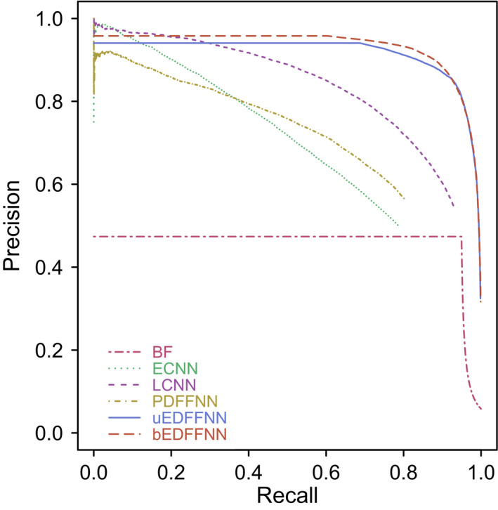
Precision‐recall curves for all possible cutoff values of the Bloom filter (BF), Eudex convolutional neural network (ECNN), letter convolutional neural network (LCNN), pseudosyllable deep feed‐forward neural network (PDFFNN), uninomial ensemble deep feed‐forward neural networks (uEDFFNN), and binomial ensemble deep feed‐forward neural networks (bEDFFNN) calculated from the validation data (5% of the total data set; not used for neural network training or testing). A 5% random error was added to the inherent BF error rate to mimic the effect of missing entries, thereby depressing the BF, uEDFFNN, and bEDFFNN curves. The bEDFFNN and uEDFFNN ensemble classifiers perform better than any of the input classifiers demonstrating complementarity.
The ensemble classifiers frequently failed to correctly identify the Latin scientific names derived from Latinized words; for example, Latin scientific eponyms with an ‘‐i’ suffix constituted approximately 10.26% of the uEDFFNN validation data set, but 13.88% of the uEDFFNN false negatives. Words that have Latin‐like construction, but are not used in Latin scientific names, were a frequent source of false positives for the ensemble classifiers; for example, within the uEDFFNN validation data set, 14.54% of the words used in Latin scientific names have an ‘‐us’ suffix, while only 0.39% of vernacular words do, but 11.34% of the uEDFFNN false positives had a ‘‐us’ suffix. Although relatively uncommon, words used in both Latin scientific names and vernacular text are also problematic (e.g., the common English word ‘are’ is also a genus of moth).
Quaesitor algorithm
The Quaesitor algorithm works by first screening plain input text with a regular expression (includes a lookahead) that captures all possible Latin binomial names in approximately canonical form, including abbreviated forms, those with embedded sectional designations, qualifiers (e.g., aff.), and nothotaxa. As a result, erroneous names are sometimes captured in minimally formatted lists. If bEDFFNN determines that a captured binomial is a Latin scientific name, the text immediately following the name is parsed to capture any infraspecific names or hybrid combinations present, which are retained or discarded based on the uEDFFNN output. The captured names are converted to a standardized format, and abbreviated genera and specific epithets are expanded where possible. Quaesitor is written in TypeScript and can be transpiled into JavaScript for interpretation within any modern web browser or using the stand‐alone NodeJS interpreter (available for Linux/Unix, MacOS, and Windows). Quaesitor can be installed via the node package manager (npm) for direct use or as a programming library for incorporation into other JavaScript/TypeScript projects.
Quaesitor performance
To evaluate the performance of Quaesitor relative to existing solutions, three test data sets were used: (1) A100, a novel synthetic data set of 100 arbitrarily selected Latin scientific names, representing a diversity of commonly encountered valid token arrangements and formats, individually embedded inside a sentence that was machine translated into each of the 16 languages that are used for >96% of biodiversity literature titles (Table 1); (2) the S800 data set of English language biological abstracts (Pafilis et al., 2013); and (3) the COPIOUS data set of Biodiversity Heritage Library extracts (Nguyen et al., 2019). The S800 and COPIOUS data set annotations were corrected, and only annotations for Latin scientific names (species and below) were evaluated. In addition to Quaesitor version 1.0.8, LINNAEUS version 2.0 (Gerner et al., 2010), SPECIES version 1.0 (Pafilis et al., 2013), TaxonFinder version 1.1.0 (Leary et al., 2007), and NetiNeti version 0.1.0 (Akella et al., 2012) were evaluated. The programs were executed in a single thread, and the analysis time (including program load time) was recorded for each document. Performance descriptive statistics and visualizations were computed with R version 3.5.3 using Precrec version 0.10.1 (Saito and Rehmsmeier, 2016) and epiR version 1.0‐4 (https://cran.r‐project.org/web/packages/epiR/index.html [accessed 29 June 2020]). The fastest program was LINNAEUS (6.7 ms/word; Fig. 2) followed by Quaesitor (8.6 ms/word), TaxonFinder (14.5 ms/word), SPECIES (34.7 ms/word), and NetiNeti (142.3 ms/word). NetiNeti has an extremely long load time and was consequently much faster (1.2 ms/word) when run as a server (i.e., when load time is disregarded). Quaesitor had both the highest recall and precision for the A100 data set (0.83 and 0.80, respectively), the highest recall and unexceptional precision for the S800 data set (0.97 and 0.84, respectively), and the highest recall and mediocre precision (0.80 and 0.69, respectively) for the COPIOUS data set (Fig. 2).
Figure 2.

Precision versus recall for the (A) A100, (B) S800, and (C) COPIOUS data sets using LINNAEUS (L), NetiNeti (N), Quaesitor (Q), SPECIES (S), and TaxonFinder (T). Error bars indicate 99% confidence intervals. Confidence area opacity indicates the relative processing time on a log scale, with darker colors indicating slower programs.
CONCLUSIONS
Quaesitor consistently had the highest recall rate of the tested solutions, making it particularly well‐suited for generating search indices (Fig. 2). In addition, Quaesitor performs well on non‐English texts (Fig. 2A); although the other tested solutions are able to find Latin scientific names within non‐English vernacular backgrounds, the error rate is unacceptably high. Due to these performance properties, Quaesitor will likely be a valuable tool for the mobilization of data contained within scanned specimen labels and biodiversity literature.
ACKNOWLEDGMENTS
Esther Jackson, Susan Lynch, and Mai Reitmeyer provided summaries of the library catalog records of the New York Botanical Garden, Biodiversity Heritage Library, and American Museum of Natural History, respectively. The City University of New York neither contributed to nor provided material support for this research in any way, yet insists that its address be included in all publications of graduate faculty.
Little, D. P. 2020. Recognition of Latin scientific names using artificial neural networks. Applications in Plant Sciences 8(7): e11378.
Data Availability
The instructions for use, computer code, trained neural networks, testing/training/validation data, and annotated text corpora can be downloaded from GitHub (https://github.com/dpl10/quaesitor; https://github.com/dpl10/quaesitor‐cli; https://github.com/dpl10/quaesitor‐web). The programming library as well as command‐line and web interfaces can be installed via the node package manager (npm). A live version of the web interface is hosted by the New York Botanical Garden (https://www.nybg.org/files/scientists/dlittle/quaesitor.html).
LITERATURE CITED
- Abadi, M. , Agarwal A., Barham P., Brevdo E., Chen Z., Citro C., Corrado G. S., et al. 2016. TensorFlow: Large‐scale machine learning on heterogeneous distributed systems. arXiv 1603.04467v2 [Preprint]. Published 16March 2016 [accessed 7 July 2020]. Available from https://arxiv.org/abs/1603.04467.
- Akella, L. M. , Norton C. N., and Miller H.. 2012. NetiNeti: Discovery of scientific names from text using machine learning methods. BMC Bioinformatics 13: 211. [DOI] [PMC free article] [PubMed] [Google Scholar]
- Berghe, E. V. , Coro G., Bailly N., Fiorellato F., Aldemita C., Ellenbroek A., and Pagano P.. 2015. Retrieving taxa names from large biodiversity data collections using a flexible matching workflow. Ecological Informatics 28: 29–41. [Google Scholar]
- Bloom, B. H. 1970. Space/time trade–offs in hash coding with allowable errors. Communications of the ACM 13: 422–426. [Google Scholar]
- Burges, C. J. C. 1998. A tutorial on support vector machines for pattern recognition. Data Mining and Knowledge Discovery 2: 121–167. [Google Scholar]
- Chorazyk, P. , Godzik M., Pietak K., Turek W., Kisiel‐Dorohinicki M., and Byrski A.. 2017. Lightweight volunteer computing platform using web workers. Procedia Computer Science 108: 948–957. [Google Scholar]
- Gerner, M. , Nenadic G., and Bergman C. M.. 2010. LINNAEUS: A species name identification system for biomedical literature. BMC Bioinformatics 11: 85. [DOI] [PMC free article] [PubMed] [Google Scholar]
- Herrera, D. , Chen H., Lavoie E., and Hendren L.. 2018. WebAssembly and JavaScript Challenge: Numerical program performance using modern browser technologies and devices. Sable Technical Report No, McLAB‐2018‐02. McGill University, School of Computer Science, Montreal, Canada. [Google Scholar]
- Jeni, L. A. , Cohn J. F., and De La Torre F.. 2013. Facing imbalanced data—Recommendations for the use of performance metrics. Proceedings of the 2013 Humaine Association Conference on Affective Computing and Intelligent Interaction, 245–251. [DOI] [PMC free article] [PubMed]
- Koning, D. , Sarkar I. N., and Moritz T.. 2005. TaxonGrab: Extracting taxonomic names from text. Biodiversity Informatics 2: 79–82. [Google Scholar]
- Kruskal, J. B. 1964. Multidimensional scaling by optimizing goodness of fit to a nonmetric hypothesis. Psychometrika 29: 1–27. [Google Scholar]
- Leary, P. R. , Remsen D. P., Norton C. N., Patterson D. J., and Sarkar I. N.. 2007. uBioRSS: Tracking taxonomic literature using RSS. Bioinformatics 23: 1434–1436. [DOI] [PubMed] [Google Scholar]
- LeCun, Y. , Bengio Y., and Hinton G.. 2015. Deep learning. Nature 521: 436–444. [DOI] [PubMed] [Google Scholar]
- Min, S. , Lee B., and Yoon S.. 2016. Deep learning in bioinformatics. Briefings in Bioinformatics 18: 851–869. [DOI] [PubMed] [Google Scholar]
- Morse, L. E. 1971. Specimen identification and key construction with time‐sharing computers. Taxon 20: 269–282. [Google Scholar]
- Naderi, N. , Kappler T., Baker C. J. O., and Witte R.. 2011. OrganismTagger: Detection, normalization and grounding of organism entities in biomedical documents. Bioinformatics 27: 2721–2729. [DOI] [PubMed] [Google Scholar]
- Nguyen, N. T. H. , Gabud R. S., and Ananiadou S.. 2019. COPIOUS: A gold standard corpus of named entities towards extracting species occurrence from biodiversity literature. Biodiversity Data Journal 7: e29626. [DOI] [PMC free article] [PubMed] [Google Scholar]
- Pafilis, E. , Frankild S. P., Fanini L., Faulwetter S., Pavloudi C., Vasileiadou A., Arvanitidis C., and Jensen L. J.. 2013. The SPECIES and ORGANISMS resources for fast and accurate identification of taxonomic names in text. PLoS ONE 8: e65390. [DOI] [PMC free article] [PubMed] [Google Scholar]
- R Core Team . 2019. R: A language and environment for statistical computing. R Foundation for Statistical Computing, Vienna, Austria: Website http://www.R‐project.org/ [accessed 29 June 2020]. [Google Scholar]
- Rebholz‐Schuhmann, D. , Arregui M., Gaudan S., Kirsch H., and Jimeno A.. 2007. Text processing through web services: Calling Whatizit. Bioinformatics 24: 296–298. [DOI] [PubMed] [Google Scholar]
- Rennie, J. D. M. , Shih L., Teevan J., and Karger D. R.. 2003. Tackling the poor assumptions of naive bayes text classifiers. Proceedings of the Twentieth International Conference on International Conference on Machine Learning, 616–623.
- Roskov, Y. , Ower G., Orrell T., Nicolson D., Bailly N., Kirk P. M., Bourgoin T., et al. [eds.]. 2018. Species 2000 & ITIS Catalogue of Life, 2018 Annual Checklist. Available at www.catalogueoflife.org/annual‐checklist/2018 [accessed 29 June 2020]. Naturalis, Leiden, the Netherlands.
- Saito, T. , and Rehmsmeier M.. 2016. Precrec: Fast and accurate precision‐recall and ROC curve calculations in R. Bioinformatics 33: 145–147. [DOI] [PMC free article] [PubMed] [Google Scholar]
- Sautter, G. , Bohm K., and Agosti D.. 2006. A combining approach to find all taxon names (FAT). Biodiversity Informatics 3: 46–58. [Google Scholar]
- Schultz, A. , Wieland R., and Lutze G.. 2000. Neural networks in agroecological modelling—Stylish application or helpful tool? Computers and Electronics in Agriculture 29: 73–97. [Google Scholar]
- Steinarsson, S. 2013. Downsampling time series for visual representation. M.S. thesis, University of Iceland, Reykjavik, Iceland. [Google Scholar]
Associated Data
This section collects any data citations, data availability statements, or supplementary materials included in this article.
Data Availability Statement
The instructions for use, computer code, trained neural networks, testing/training/validation data, and annotated text corpora can be downloaded from GitHub (https://github.com/dpl10/quaesitor; https://github.com/dpl10/quaesitor‐cli; https://github.com/dpl10/quaesitor‐web). The programming library as well as command‐line and web interfaces can be installed via the node package manager (npm). A live version of the web interface is hosted by the New York Botanical Garden (https://www.nybg.org/files/scientists/dlittle/quaesitor.html).