Estimating the relative probability of direct transmission between infectious disease patients

Abstract

Background

Estimating infectious disease parameters such as the serial interval (time between symptom onset in primary and secondary cases) and reproductive number (average number of secondary cases produced by a primary case) are important in understanding infectious disease dynamics. Many estimation methods require linking cases by direct transmission, a difficult task for most diseases.

Methods

Using a subset of cases with detailed genetic and/or contact investigation data to develop a training set of probable transmission events, we build a model to estimate the relative transmission probability for all case-pairs from demographic, spatial and clinical data. Our method is based on naive Bayes, a machine learning classification algorithm which uses the observed frequencies in the training dataset to estimate the probability that a pair is linked given a set of covariates.

Results

In simulations, we find that the probabilities estimated using genetic distance between cases to define training transmission events are able to distinguish between truly linked and unlinked pairs with high accuracy (area under the receiver operating curve value of 95%). Additionally, only a subset of the cases, 10–50% depending on sample size, need to have detailed genetic data for our method to perform well. We show how these probabilities can be used to estimate the average effective reproductive number and apply our method to a tuberculosis outbreak in Hamburg, Germany.

Conclusions

Our method is a novel way to infer transmission dynamics in any dataset when only a subset of cases has rich contact investigation and/or genetic data.

Key Messages

• This paper introduces a method to calculate the relative probability that two infectious disease patients are connected by direct transmission using clinical, demographic, geographical and genetic characteristics.

• We use naive Bayes, a machine learning technique, to estimate these probabilities using a training set of probable links defined by contact investigation and/or pathogen whole genome sequence data on a subset of cases.

• These probabilities can be used to explore possible transmission chains, rule out transmission events and estimate the reproductive number.

Introduction

Infectious disease parameters such as the serial interval (time between symptom onset from primary to secondary case) and the reproductive number (average number of secondary cases produced by a primary case over the infection course) are instrumental in managing outbreaks.¹ For diseases in which disease progression shortly follows infection, these parameters have been studied extensively.^1–6 For others, such as tuberculosis (TB), the serial interval and reproductive number estimates are few and inconsistent.^7–9

Serial interval and reproductive number estimation methods often rely on determining which cases are linked by direct transmission. Pathogen whole genome sequence (WGS) data are a powerful tool to link cases, and several methods have been developed to analyse these data.^10–22 However, WGS data are still relatively expensive and require bioinformatics expertise, making universal use in high disease burden settings unfeasible. Therefore, datasets may have WGS data on only a proportion of cases. Another way to link cases is contact investigations, which are often part of an outbreak response.^23–29 However, these investigations do not perfectly identify infectors due to nonspecific transmission mechanisms, disease characteristics and the willingness and ability of cases to share contact information.^26,29–33 Additionally, contact investigations are time consuming and require significant human resources, again meaning that these data are unlikely to be available for all cases.

Here, we present a novel method to predict the relative probability of direct transmission between infectious disease patients using pathogen WGS data and/or contact investigations when these data are only available on a proportion of cases, paired with other risk factor data. These probabilities can be used to understand outbreak transmission dynamics and estimate the reproductive number without a reliable serial interval estimate. We apply our method to a TB outbreak in Hamburg, Germany.

Methods

Data structure

Our method requires individual-level case data, e.g. geographical location, clinical information, demographics and observation date. At least a subset of the cases needs additional information, e.g. detailed contact investigation and/or pathogen genome WGS data, to form the training set to generate the model. We transform this dataset of individuals into a dataset of ordered case-pairs ($i,\mathrm{ }j$), where case $i$ was observed before case $j$. We convert the individual-level covariates (${\mathrm{X}}_1,\mathrm{ }{\mathrm{X}}_2,\mathrm{ }\dots ,\mathrm{ }{\mathrm{X}}_{\mathrm{p}}$) into pair-level covariates ($Z_1,\mathrm{ }{Z}_2,\mathrm{ }\dots ,\mathrm{ }{Z}_p$) by computing ‘distances’ which capture how well the individuals match on covariate values. For example, if the individual-level covariate $X_1$ was town of residence, the pair-level covariate $Z_1$ could indicate if the individuals live in the same town, neighbouring towns or more distant towns (see Supplementary Methods available as Supplementary data at IJE online).

Naive Bayes

To estimate the probability that cases $i$ and $j$ are linked by direct transmission, $p(i\to j$), we use a classification technique called naive Bayes. This method uses Bayes rule to estimate the probability of an outcome given a set of covariates from the observed frequencies in a training dataset. Our outcome, $L_{ij}$ equals 1 if case $i$ infected case $j$ and 0 otherwise. We know the probable value of $L_{ij}$ for case-pairs in the training set based on pathogen WGS and/or contact investigation data, and want to predict the probability that $L_{ij}=1$ for the remaining pairs.

We first use the training set to calculate $P(Z_k=z_k|L=l)$, the probability that the pair-level covariate $Z_k$ equals $z_k$ for each covariate $k\in \{1,\mathrm{ }2,\mathrm{ }\dots ,\mathrm{ }p\}\mathrm{ }$for a pair with link status $l\in \{1,\mathrm{ }0\}$, using:

$$\begin{array}{c}P(Z_k=z_{k}L=l)=\frac{{\sum }_{i,j}\mathbb{1}\left\{L_{ij}=l,\mathrm{ }{Z}_{\mathit{kij}}=z_k\right\}+\alpha }{{\sum }_{i,j}\mathbb{1}\left\{L_{ij}=l\right\}+\alpha n_k}. \end{array}$$ (1)

The indicator function, $\mathbb{1}$, equals 1 if the input is true and 0 if false, $n_k$ is the number of levels of $Z_k$ for $k\in \{1,\mathrm{ }2,\mathrm{ }\dots ,\mathrm{ }p\}$, and $\alpha$ is a smoothing parameter to avoid zero-probabilities resulting from sparse data. The numerator, ${\sum }_{i,j}\mathbb{1}\{L_{ij}=l,\mathrm{ }{Z}_{\mathit{kij}}=z_k\}$, counts how often a pair $i,\mathrm{ }j$ has linked status $l$ and value $z_k$ for covariate $Z_k$, $k\in \{1,\mathrm{ }2,\mathrm{ }\dots ,\mathrm{ }p\}$. The denominator counts the number of pairs with link status $l$ plus the total added because of the smoothing correction ($\alpha n_k$). Then we use the training set to calculate $P(L\mathrm{ }=\mathrm{ }\mathrm{l})$, the prior probability of link status for $l\in \{1,\mathrm{ }0\}$ using:

$$\begin{array}{c}P\left(L=l\right)=\frac{{\sum }_{i,j}\mathbb{1}\left\{L_{ij}=l\right\}+\alpha }{N+2\alpha } \end{array}$$ (2)

where $N$ is the total number of cases in the training set. We used an $\alpha$ value of 1, which is equivalent to the Bayesian estimate of the probabilities in Equations 1 and 2 with a uniform prior.^34–36

We then use Bayes rule to calculate the predicted probability that case $i$ infected case $j$, $p(i\to j)$ for all pairs in the prediction set as:

$$\begin{array}{c}p\left(i\to j\right)={\mathrm{P}(\mathrm{L}}_{\text{ij}}=1{|\mathrm{Z}}_{1\text{ij}}={ \mathrm{z}}_1, \dots ,{ \mathrm{Z}}_{\text{pij}}={\mathrm{z}}_{\mathrm{p}})\\ =\frac{\mathrm{P}\left({\mathrm{Z}}_1={ \mathrm{z}}_1, \dots ,{ \mathrm{Z}}_{\mathrm{p}}={\mathrm{z}}_{\mathrm{p}}|\mathrm{L}=1\right)\mathrm{P}\left(\mathrm{L}=1\right)}{\mathrm{P}\left({\mathrm{Z}}_1={\mathrm{z}}_1, \dots ,{ \mathrm{Z}}_{\mathrm{p}}={\mathrm{z}}_{\mathrm{p}}\right)} \\ =\frac{{\prod }_{k=1}^p\mathrm{P}({\mathrm{Z}}_{\mathrm{k}}={\mathrm{z}}_{\mathrm{k}}|\mathrm{L}=1)\mathrm{P}(\mathrm{L}=1) }{{\prod }_{k=1}^p\mathrm{P}({\mathrm{Z}}_{\mathrm{k}}={\mathrm{z}}_{\mathrm{k}}|\mathrm{L}=1)\mathrm{P}(\mathrm{L}=1)+{\prod }_{k=1}^p\mathrm{P}({\mathrm{Z}}_{\mathrm{k}}={\mathrm{z}}_{\mathrm{k}}|\mathrm{L}=0)\mathrm{P}(\mathrm{L}=0)}.\end{array}$$ (3)

We calculate the conditional probability of all covariate values given link status$\mathrm{ }\mathrm{P}({\mathrm{Z}}_1=\mathrm{ }{\mathrm{z}}_1,\mathrm{ }\dots ,\mathrm{ }{\mathrm{Z}}_{\mathrm{p}}={\mathrm{z}}_{\mathrm{p}}|\mathrm{L} = 1)$, as the product of the conditional probabilities of each covariate,$\mathrm{ }\mathrm{P}({\mathrm{Z}}_{\mathrm{k}}={\mathrm{z}}_{\mathrm{k}}|\mathrm{L} = 1)$ for $k\in \{1,\mathrm{ }2,\mathrm{ }\dots ,\mathrm{ }p\}$, assuming that covariates are conditionally independent.

Finally, we scale the estimated probabilities to represent the relative likelihood that case $j$ has been infected by case $i$ rather than any other sampled case, using:

$$\begin{array}{c}p{\left(i\to j\right)}^s=\frac{p\left(i\to j\right)}{{\sum }_{m\ne j}p\left(m\to j\right)}. \end{array}$$ (4)

We call this scaled probability, $p{\left(i\to j\right)}^s$, the ‘relative transmission probability’. Note: the ordered nature of the pair dataset implies that if case $j$ was observed before case $i$, then $p\left(i\to j\right)=0$.

Training dataset construction

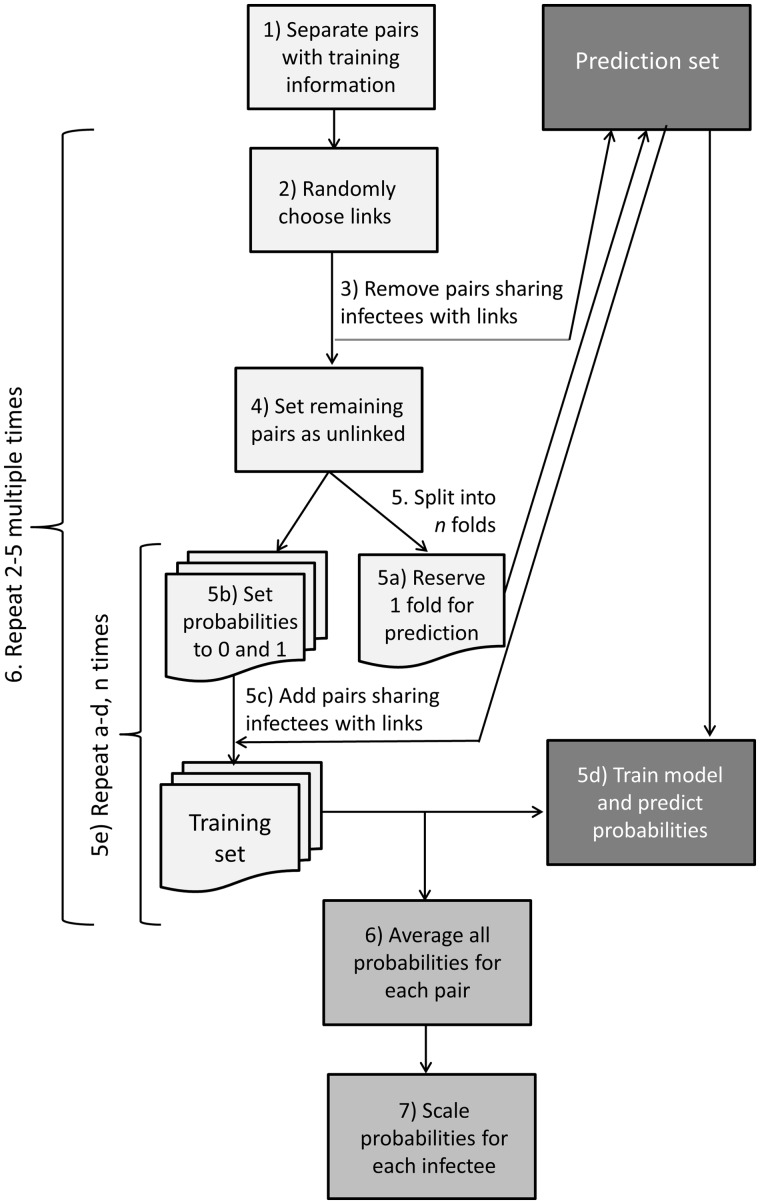
Naive Bayes uses a training set with a known outcome to inform a model to estimate probabilities in a separate prediction set. In our training set however, the outcome represents probable rather than certain transmission events, inferred from a subset of cases with pathogen WGS and/or detailed contact investigation data. Because of this uncertainty, we want to estimate the transmission probability of the training case-pairs as well as those that lack WGS or contact data. Therefore, we use an iterative estimation procedure where each pair has a turn in the prediction set. The algorithm used to create the training set and iterative estimation procedure is diagrammed in Figure 1 and described further in the Supplementary Methods available as Supplementary data at IJE online.

Figure 1.

Flowchart depicting the algorithm we used to create the training dataset and the iterative procedure to estimate the relative transmission probabilities.

Reproductive number estimation

To estimate the reproductive number, we use the Wallinga and Teunis approach³ which calculates the relative probability that each case was infected by all other cases, using the serial interval distribution. The effective reproductive number ($R_i$) for each case is then calculated by summing the scaled probabilities for all possible infectees with:

$$\begin{array}{c}{\mathrm{R}}_{\mathrm{i}}={\sum }_{m\ne i}{p\left(i\to m\right)}^S \end{array}$$ (5)

assuming that all cases are sampled, and the outbreak is completed. We use this equation, but with probabilities derived from our naive Bayes approach.

By averaging the individual reproductive numbers for all cases observed at each time point, we obtain time-level effective reproductive number ($R_t$) estimates and average those values for the stable portion of the outbreak, to give an average reproductive number estimate over the study period (${\overline{R}}_t$). We calculate confidence intervals for $R_t$ and ${\overline{R}}_t$ using parametric bootstrapping (see Supplementary Methods available as Supplementary data at IJE online).

Simulation study

We assess our method by using an R package called TransPhlyo, developed by Didelot et al.,²¹ to simulate 1000 outbreaks of at least 500 cases with TB transmission dynamics and composed of multiple transmission chains.^11,37 We simulate each transmission chain with an ${\overline{R}}_t$ of 1.2 and a shifted gamma distributed generation interval (shape = 1.05, scale = 2.0, shift = 0.25) so at least 3 months separated each transmission event (Ma et al., in press at AJE). We simulate representative pathogen genomes and inform the model with four different covariates, representing clinical and demographic variables and a discretized version of the time between infection. We order cases by the date of infection.

We compare our method performance when training using probable transmission events defined by single nucleotide polymorphism (SNP) distances, with performance when training using truly linked and unlinked case-pairs. We also compare the performance with that of probabilities derived from the time between infection dates and the serial/generation interval distribution motivated by the Wallinga and Teunis method.³ For each simulation scenario (Box 1), we calculate the area under the receiver operating curve (AUC), assess how the probability of the true infector rank compares with the probabilities of all possible infectors and estimate ${\overline{R}}_t$. To determine what proportion of cases needs to be in the training set to achieve good performance, we use a sensitivity analysis with various outbreak sizes and training proportions. We also assess the performance when using the date of observation instead of the date of infection to order the cases. The simulation structure is explained further in the Supplementary Methods available as Supplementary data at IJE online.

Box 1. Description of simulation scenarios

Simulation scenarios
Model trained on true links
Model trained on SNPa distance links
Correct serial interval—gamma (1.05, scale = 2.0)
Wide serial interval—gamma (1.30, scale = 3.3)
Narrow serial interval—gamma (0.54, scale = 1.9)
Random probabilities

^aSingle nucleotide polymorphism.

Hamburg TB outbreak application

We apply our method to a small TB outbreak in Hamburg and Schleswig-Holstein, Germany, analysed in Roetzer et al.¹⁰ The outbreak includes 86 individuals from the largest strain cluster in a long-term surveillance study conducted by the health departments in these cities. The dataset includes pathogen WGS data for all individuals as well as clinical, demographic and social risk factor data. Furthermore, a subset of these individuals was involved in contact investigations performed by the local health authorities.

We define probable links in the training set in two ways: (i) SNP distances, and (ii) contact investigation. When training with SNP distance, case-pairs with <2 SNPs are considered linked and those with >12 SNPs are considered unlinked. Pairs with 2–12 SNPs are excluded from the training set as indeterminate.^11,37 When using contact investigation data, pairs who had confirmed contact with each other are considered linked, pairs without confirmed contact are considered unlinked and cases who did not undergo contact investigation are excluded. For comparison, we also calculate the relative transmission probabilities randomly and using the same serial intervals as the simulation study. We also tested different smoothing parameters, $\alpha$, to assess the possible impact of adding one to each cell on the estimate of ${\overline{R}}_t$.

We implemented the method to calculate relative transmission probabilities and estimate the reproductive number in an R package, nbTransmission, available from [https://github.com/sarahleavitt/nbTransmission]. Additionally, the code used to produce the simulations, analyse the Hamburg outbreak and produce all results reported in this paper is also available on GitHub at [https://github.com/sarahleavitt/nbSimulation and https://github.com/sarahleavitt/nbPaper1].

Results

Simulation study

The sample sizes of the 1000 outbreaks (which were simulated to have at least 500 cases) ranged 500–1178 (median: 545). Each outbreak had 2–39 (median: 14) transmission chains with 2–846 (median: 9) cases each. Supplementary Figure S1, available as Supplementary data at IJE online, shows the relative transmission probability distributions for one outbreak comparing truly linked and unlinked case-pairs. In that outbreak, our method estimated relative transmission probabilities of <0.005 for most unlinked pairs (92% when training with the truth and 89% training using SNP distance). With both ways of defining the training set, our method assigned more than 75% of truly linked case-pairs higher probabilities than the serial interval method (Supplementary Figure S2, available as Supplementary data at IJE online).

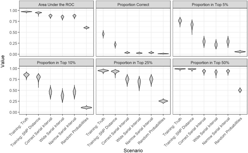
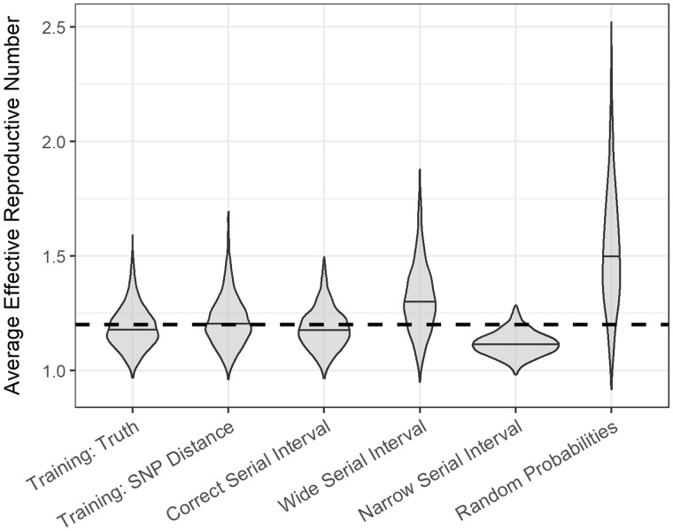
Over 1000 simulations, the average AUC was 97% [standard deviation (SD) 0.6] compared with 95% (SD 1.2) when the model was trained using true links and SNP distances, respectively (Figure 2; Supplementary Table S1, available as Supplementary data at IJE online). When the model was trained with links determined by SNP distances, the estimated probability of the true infector was the highest of all possible infectors 22% of the time and ranked in the top 25% of all possible infectors 93% (SD 2.4) of the time [compared with 46% (SD 2.6) and 95% (SD 1.6) when training with true links]. Our method outperformed probabilities estimated using serial intervals (Figure 2; Supplementary Table S1, available as Supplementary data at IJE online). Figure 3, and Supplementary Table S2 (available as Supplementary data at IJE online), show the ${\overline{R}}_t$ estimates for each of the different scenarios compared with the 1.2 value used to simulate the outbreaks. Both our method and the correct serial interval estimated ${\overline{R}}_t$ accurately. However, when incorrect serial intervals were used, the ${\overline{R}}_t$ estimates were either too high or too low.

Figure 2.

Violin plots of the performance metrics for the different scenarios across 1000 simulated outbreaks. The scenarios were: our method with a training set of true links; our method with a training set of links defined by single nucleotide polymorphism (SNP) distance; probabilities derived from the serial interval distribution used to simulate the outbreak: gamma(1.05, 2.0); probabilities derived from a serial interval distribution that is too wide: gamma(1.3, 3.3) and too narrow: gamma(0.54, 1.9); and random probabilities. The metrics shown are the area under the receiver operating curve (AUC), the proportion of time the true infector was assigned the highest relative transmission probability (Proportion Correct), and the proportion of time the probability of the true infector was ranked in the top 5%, 10%, 25%, and 50% of all possible infectors.

Figure 3.

Violin plots of the distribution of the average effective reproductive number for different scenarios across 1000 simulated outbreaks. The dashed horizontal line indicates the true value of 1.2 that was used to simulate the outbreaks.

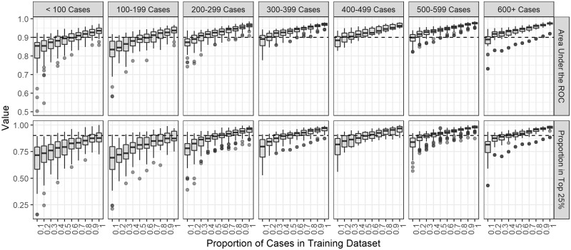
In our sensitivity analysis, the performance improved and the metrics’ variability decreased as the proportion of cases in the training set increased (Supplementary Figure S3, available as Supplementary data at IJE online). If the sample size was at least 500, only 10% of all cases were needed to train the model to obtain good performance. For a sample size of 200–500, training the model with 20% of cases resulted in good performance. For smaller outbreaks, the performance was best with at least 50% of the cases in the training set (Figure 4). The ${\overline{R}}_t$ estimates grew increasingly accurate as the training dataset proportion increased (Supplementary Figure S4, available as Supplementary data at IJE online). We also found that there was little change in the performance when using the observation date instead of the infection date (Supplementary Figure S5, available as Supplementary data at IJE online).

Figure 4.

Boxplots of the performance metrics by training set proportion in 300 simulated outbreaks stratified by the total sample size of the outbreak. The metrics shown are the area under the receiver operating curve (ROC) and the proportion of time the relative transmission probability of the true source case was ranked in the top 25%. The dotted black line indicates a value of 90% on either metric.

Hamburg TB outbreak application

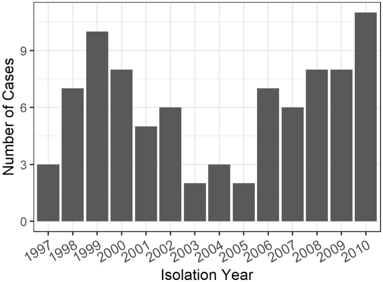
Case counts over the course of the Hamburg outbreak and clinical and demographic characteristics are shown in Figure 5 and Table 1. The 86 cases resulted in 3633 possible ordered case-pairs where the possible infector was observed before the infectee. These pairs were separated by 0–20 SNPs (median: 4). Of the 86 individuals, 31 (36%) were part of contact investigations, with 51 confirmed contacts. All individual-level covariates were transformed into pair-level covariates (Table 2).

Figure 5.

Case counts by year for the Hamburg outbreak described in Roetzer et al.¹⁰.

Table 2.

Pair-level demographic and clinical characteristics for the Hamburg outbreak

Covariate	Level	n (%) of all pairs
		(n = 3633)
City	Same city	2148 (59.1%)
	Different city	1485 (40.9%)
Nationality	Both German	2129 (58.6%)
	Same foreign country	19 (0.5%)
	One German, one foreign country	1315 (36.2%)
	Different foreign countries	170 (4.7%)
Sex	Male to male	2401 (66.1%)
	Female to female	120 (3.3%)
	Male to female	757 (20.8%)
	Female to male	355 (9.8%)
Age group	Same age group	695 (19.1%)
	Different age group	2938 (80.9%)
Smear status	Infector smear–	2339 (64.4%)
	Infector smear+	1294 (35.6%)
HIVa status	Infector HIV–	3463 (95.3%)
	Infector HIV+	170 (4.7%)
Substance abuse	Both yes	1372 (37.8%)
	Both no	526 (14.5%)
	Different	1735 (47.8%)
Residence	Both permanent	2473 (68.1%)
	Both homeless	105 (2.9%)
	Different	1055 (29.0%)
Affiliation to alcohol-consuming milieu/street scene	Both affiliated	2062 (56.8%)
	Both not affiliated	210 (5.8%)
	Different	1361 (37.5%)
Observation time difference	<1 year	546 (15.0%)
	1–2 years	485 (13.3%)
	2–3 years	374 (10.3%)
	3–4 years	305 (8.4%)
	>4 years	1923 (52.9%)
SNPb distance	<2 SNPs	796 (21.9%)
	2–12 SNPs	2452 (67.5%)
	>12 SNPs	385 (10.6%)
Confirmed contact	Yes	51 (1.4%)
	No	408 (11.2%)
	Unknown	3174 (87.4%)

^aHuman immunodeficiency virus.

^bSingle nucleotide polymorphism.

Table 1.

Individual-level demographic and clinical characteristics for the Hamburg outbreak

Covariate	Level	n (%) of all individuals
		(n = 86)
City	Hamburg	62 (72.1%)
	Schleswig-Holstein	24 (27.9%)
Nationality	German	66 (76.7%)
	Other	20 (23.3%)
Sex	Female	16 (18.6%)
	Male	70 (81.4%)
Age group	<25 years old	5 (5.8%)
	25–34 years old	13 (15.1%)
	35–44 years old	24 (27.9%)
	45–54 years old	20 (23.3%)
	55–64 years old	16 (18.6%)
	≥65 years old	8 (9.3%)
Smear status	Negative	50 (58.1%)
	Positive	36 (41.9%)
HIVa status	Negative	81 (94.2%)
	Positive	5 (5.8%)
Substance abuse	No	33 (38.4%)
	Yes	53 (61.6%)
Residence	Permanent residence	71 (82.6%)
	Homeless	15 (17.4%)
Affiliation to alcohol-consuming milieu/street scene	Not affiliated	21 (24.4%)
	Affiliated	65 (75.6%)

^aHuman immunodeficiency virus.

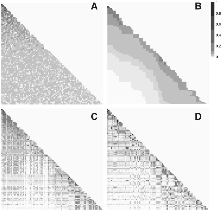
Figure 6 shows heatmaps of all potential infectors using our method compared with random probabilities (Figure 6A) and a serial interval distribution (Figure 6B). Using our method, defining links with either SNP distance (Figure 6C) or confirmed contact (Figure 6D), there is more variation in the relative transmission probability across possible infectors than the serial interval or random scenarios. Some infectees have infectors with a higher probability than all others in the row, suggesting this is the likely true infector. However, even for rows without a clear infector, many of the possible infectors have very low probabilities and can be eliminated.

Figure 6.

Heatmaps of the relative probabilities that each infectee (rows) was infected by each possible infector (columns) in the Hamburg TB outbreak. Darker squares represent higher probabilities. The cases are ordered by infection date, with the earliest cases on the top and to the left. Each panel shows the results from a different method of calculating probabilities: A) randomly assigned probabilities; B) probabilities calculated using a gamma(1.05, 2.0) serial interval distribution; C) probabilities calculated using our method and a training set with links based on single nucleotide polymorphism (SNP) distance; and D) probabilities calculated using our method and a training set with links based on contact investigations.

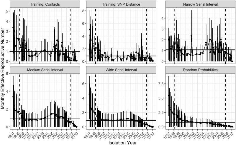
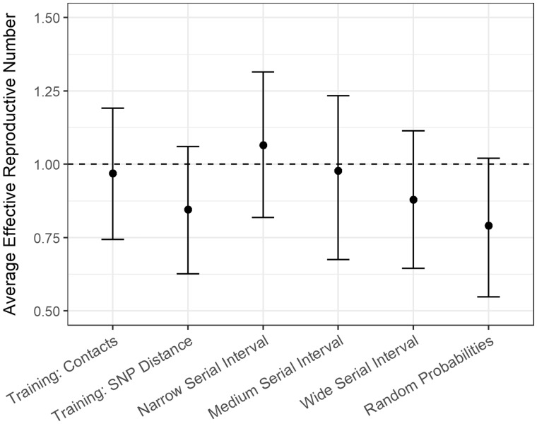
All methods except random probabilities show spikes in$\mathrm{ }{R}_t$ at the second peak in case counts, but to different degrees (Figure 7). The ${\overline{R}}_t$ estimate was 0.97 [95% confidence interval (CI) 0.73–1.19] when training with confirmed contacts and 0.85 (95% CI 0.63–1.07) when training with SNP distances (Figure 8;Supplementary Table S3, available as Supplementary data at IJE online,). Changing the smoothing parameter, $\alpha$, had negligible effect on these estimates (Supplementary Table S4, available as Supplementary data at IJE online).

Figure 7.

Monthly reproductive number over the course of the 14 years of the Hamburg TB outbreak estimated from the relative transmission probabilities with bootstrap confidence intervals. Each panel shows the results from a different method of calculating probabilities: our method and a training set with links based on contact investigation data; our method and a training set with links based on single nucleotide polymorphism (SNP) distance; probabilities derived from narrow: gamma(0.54, 1.9), medium: gamma(1.05, 2.0) and wide: gamma(1.33, 3.0) serial interval distributions; and random probabilities. The months in between the dotted horizontal lines were averaged to find the average effective reproductive number for the scenario which is shown by the solid horizontal line.

Figure 8.

Average effective reproductive number for the Hamburg TB outbreak calculated using the relative transmission probabilities derived from different methods of calculating probabilities: our method and a training set with links based on contact investigation data; our method and a training set with links based on single nucleotide polymorphism (SNP) distance; probabilities derived from narrow: gamma(0.54, 1.9), medium: gamma(1.05, 2.0) and wide: gamma(1.33, 3.0) serial interval distributions; and random probabilities. The vertical bars represent 95% bootstrap confidence intervals. The dotted horizontal line represents an average effective reproductive number of 1.

Discussion

We have developed a method to estimate the relative transmission probability between pairs of infectious disease cases using clinical, demographic, geographical and genetic data, which accurately distinguishes between linked and unlinked case-pairs. Using an SNP distance proxy for transmission to train the model, the classification accuracy was 95%, and 93% of the time the true infector had a probability in the top 25% of all possible infectors. Therefore, our method provides a powerful way to rule out transmission events, outperforming the serial interval method in all metrics and accurately estimating ${\overline{R}}_t$. This is important because the serial interval is difficult to estimate and highly variable,^7,8,38 highlighting the value of estimation methods that are independent of the serial interval.

Applying our method to the Hamburg outbreak, we found that both ways of model training allowed for the elimination of many transmission links. The training methods produced slightly different ${\stackrel{-}{R}}_t$ estimates, which is expected because neither of the probable transmission events used to train the model perfectly capture the truth. Using contact investigation for training is more discriminating than SNP distance, because we know the cases have interacted but we may miss links with unknown or unreported contacts. Using SNP distances for training will result in fewer missed links, but could connect cases that never had contact with one another. We hypothesize that the true reproductive number for M. tuberculosis in this context lies in between these two estimates (0.85–0.97). We recognize however, that for TB, reactivation risk and long time-frames may limit the usefulness of this conventional ${\overline{R}}_t$ estimate. Our method is applicable to outbreaks of diseases other than tuberculosis. Method performance depends on how likely the training links are true links and therefore will perform better with faster mutating pathogens or rich contact investigations.

Most established methods for exploring transmission focus on either identifying recent transmission clusters,^{11,14,37,39–42} recreating possible transmission chains^{12,13,15–20,43–45} or identifying the true infector.^46–50 When estimating transmission parameters, simply knowing clusters is not informative enough and identifying the true infector is often impossible. The strength of our method is that it directly estimates the relative transmission probability for all case-pairs, instead of seeking to find the true infector or a set of possible transmission trees. This gives our method broad applicability as it can identify potential true infectors (pairs with very high probabilities) or transmission clusters (groups of pairs with high probabilities). These probabilities can then be used to estimate transmission parameters incorporating the uncertainty around the true infector.

If all cases in an outbreak have WGS data, numerous powerful analytical methods have been developed to analyse transmission dynamics and estimate transmission probabilities which also can incorporate covariates.^21,22,39 Teunis et al. developed a way to estimate transmission probabilities without relying on WGS data, but it requires prior knowledge of the relationship between the covariates and transmission.⁵¹ Our method’s use of training and prediction sets means that not all cases require highly discriminatory information such as WGS data to estimate relative transmission probabilities. This is relevant because existing datasets often have rich demographic, clinical and spatial data but lack detailed contact investigation or pathogen WGS data due to the significant time and resources needed to obtain these data. Provided a subset of cases, 10–50% depending on the sample size, has this information, our method can infer transmission patterns among the remaining cases as well. Additionally, our method does not assume any relationship between covariates and transmission.

Our method is based on naive Bayes, a simple but powerful machine learning tool that has many diverse applications.^{34,35,52–54} We preferred naive Bayes to logistic regression or other more complex machine learning algorithms due to its simplicity and ease of incorporating missing values and sparse data. Although traditionally a naive Bayes model is trained with a set of true events, our method performs almost as well when SNP distance is used as a transmission proxy. Though it has many advantages, the method also makes assumptions. First, naive Bayes assumes independence of the covariates when conditioning on the outcome, which may not be realistic. However, numerous papers have shown that naive Bayes still performs well even when this assumption is violated.^53,55–57 Furthermore, many naive Bayes extensions have been developed which relax this assumption,^35,58,59 which could be easily integrated into our method.

The Wallinga and Teunis³ approach for estimating ${\overline{R}}_t$ we used assumes that every case was infected by someone who has been sampled. These authors and others found that simulations incorporating random incomplete reporting did not substantially decrease the accuracy of their ${\stackrel{-}{R}}_t$ estimates, so this is unlikely to be an issue here.^3,60 Our probability estimates themselves do not assume that all cases in an outbreak are sampled, because we estimate the relative probability that one case was infected by another over any other sampled case. If the infector for a case was not sampled, our method may assign a high transmission probability to another case, but this should be interpreted as relative to all sampled cases as opposed to the absolute probability that this case is the true infector. Our method could also be affected by biased sampling, e.g. because only certain types of cases are observed or have the information needed to define training links. Future work could more fully examine the effect of biased reporting and biased training sets.

Finally, as with other infectious disease analytical approaches, our method assumes that cases were infected in the same order as that in which they were observed.^42,61 Although not a strong assumption for diseases with clear symptoms and a short latent period, this may not be appropriate for diseases such as TB, with a highly variable, potentially long latent period and often substantial delays in care-seeking and diagnosis.^62,63 Although this assumption is a known problem in infectious disease research, it is frequently made,^46,47 and we found that using the observation date instead of the infection date in our simulations did not substantially change our results.

We have developed a method to estimate the relative transmission probabilities between pairs of cases which is flexible, using any information sources that are available without making assumptions about the relationship between these covariates and transmission. The power of our method is that only a subset of cases requires pathogen WGS or contact investigation data, making this method applicable to many outbreak and surveillance datasets. These probabilities can be used to better understand the transmission dynamics of an outbreak by identifying or ruling out possible transmission events and estimating transmission parameters. In a disease where determining transmission events can be extremely difficult, using transmission probabilities between all possible cases provides a unique and powerful analysis tool.

Supplementary Data

Supplementary data are available at IJE online.

Funding

This work was supported by the US National Institutes of Health [NIHGMS R01GM122876]. S.V.L. was also funded by the Interdisciplinary Training grant from the US National Institutes of Health [NIHGMS T32GM074905]. H.E.J. was also funded by US National Institutes of Health [NIH K01AI102944]. C.R.H. and L.F.W. were also funded by the Providence/Boston Center for AIDS Research [P30AI042853]. C.R.H. was supported by the Boston University/Rutgers Tuberculosis Research Unit [U19AI111276] and the U.S.-India Vaccine Action Program (VAP) Initiative on Tuberculosis (CRDF Global/NIAID). R.S.L. holds a Fellowship from the Canadian Institutes of Health Research [MFE-152448]. The content of the article is solely the responsibility of the authors and does not necessarily represent the views of the National Institute of Allergy and Infectious Disease or the Office of the Director, NIH. The funders had no role in the decision to publish this manuscript.

References

- 1. Boelle P-Y, Ansart S, Cori A, Valleron A-J.. Transmission parameters of the A/H1N1 (2009) influenza virus pandemic: a review. Influenza Other Respir Viruses 2011;5:306–16. [DOI] [PMC free article] [PubMed] [Google Scholar]
- 2. Riley S, Fraser C, Donnelly CA. et al. Transmission dynamics of the etiological agent of SARS in Hong Kong: impact of public health interventions. Science 2003;300:1961–67. [DOI] [PubMed] [Google Scholar]
- 3. Wallinga J, Teunis P.. Different epidemic curves for severe acute respiratory syndrome reveal similar impacts of control measures. Am J Epidemiol 2004;160:509–16. [DOI] [PMC free article] [PubMed] [Google Scholar]
- 4. Chowell G, Hengartner NW, Castillo-Chavez C, Fenimore PW, Hyman JM.. The basic reproductive number of Ebola and the effects of public health measures: the cases of Congo and Uganda. J Theor Biol 2004;300:1961–66. [DOI] [PubMed] [Google Scholar]
- 5. White LF, Pagano M.. A likelihood-based method for real-time estimation of the serial interval and reproductive number of an epidemic. Stat Med 2008;27:2999–3016. [DOI] [PMC free article] [PubMed] [Google Scholar]
- 6. Fraser C, Donnelly CA, Cauchemez S. et al. ; WHO Rapid Pandemic Assessment Collaboration. Pandemic potential of a strain of influenza A (H1N1): early findings. Science 2009;324:1557–61. [DOI] [PMC free article] [PubMed] [Google Scholar]
- 7. Ma Y, Horsburgh CR Jr,, White LF, Jenkins HE.. Quantifying TB transmission: a systematic review of reproductive number and serial interval estimates for tuberculosis. Epidemiol Infect 2018;146:1478–94. [DOI] [PMC free article] [PubMed] [Google Scholar]
- 8. Vink MA, Christoffel M, Bootsma J, Wallinga J.. Systematic reviews and meta- and pooled analyses serial intervals of respiratory infectious diseases: a systematic review and analysis. Am J Epidemiol 2014;180:865–75. [DOI] [PubMed] [Google Scholar]
- 9. Delamater PL, Street EJ, Leslie TF, Yang YT, Jacobsen KH.. Complexity of the basic reproduction number (R0). Emerg Infect Dis 2019;25:1–4. [DOI] [PMC free article] [PubMed] [Google Scholar]
- 10. Roetzer A, Diel R, Kohl TA. et al. Whole genome sequencing versus traditional genotyping for investigation of a Mycobacterium tuberculosis outbreak: a longitudinal molecular epidemiological study. PLoS Med 2013;10:e1001387. [DOI] [PMC free article] [PubMed] [Google Scholar]
- 11. Walker TM, Ip CLC, Harrell RH. et al. Whole-genome sequencing to delineate Mycobacterium tuberculosis outbreaks: a retrospective observational study. Lancet Infect Dis 2013;13:137–46. [DOI] [PMC free article] [PubMed] [Google Scholar]
- 12. Lee RS, Radomski N, Proulx J. et al. Population genomics of Mycobacterium tuberculosis in the Inuit. Proc Natl Acad Sci U S A 2015;112:13609–14. [DOI] [PMC free article] [PubMed] [Google Scholar]
- 13. Cottam EM, Thebaud G, Wadsworth J. et al. Integrating genetic and epidemiological data to determine transmission pathways of foot-and-mouth disease virus. Proc R Soc B 2008;275:887–95. [DOI] [PMC free article] [PubMed] [Google Scholar]
- 14. Didelot X, Eyre DW, Cule M. et al. Microevolutionary analysis of Clostridium difficile genomes to investigate transmission. Genome Biol 2013;13:R118. [DOI] [PMC free article] [PubMed] [Google Scholar]
- 15. Jombart T, Cori A, Didelot X, Cauchemez S, Fraser C, Ferguson N.. Bayesian reconstruction of disease outbreaks by combining epidemiologic and genomic data. PLoS Comput Biol 2014;10:e1003457. [DOI] [PMC free article] [PubMed] [Google Scholar]
- 16. Long SW, Beres SB, Olsen RJ, Musser M.. Absence of patient-to-patient intrahospital transmission of Staphylococcus aureus as determined by whole-genome sequencing. MBio 2014;5:1–10. [DOI] [PMC free article] [PubMed] [Google Scholar]
- 17. Morelli MJ, Thébaud G, Chadœuf J, King DP, Haydon DT, Soubeyrand S.. A Bayesian inference framework to reconstruct transmission trees using epidemiological and genetic data. PLoS Comput Biol 2012;8:e1002768. [DOI] [PMC free article] [PubMed] [Google Scholar]
- 18. Worby CJ, O’Neill PD, Kypraios T. et al. Reconstructing transmission trees for communicable diseases using densely sampled genetic data. Ann Appl Stat 2016;10:395–417. [DOI] [PMC free article] [PubMed] [Google Scholar]
- 19. Ypma RJF, Bataille AMA, Stegeman A, Koch G, Wallinga J, van Ballegooijen WM.. Unravelling transmission trees of infectious diseases by combining genetic and epidemiological data. Proc R Soc B 2012;279:444–50. [DOI] [PMC free article] [PubMed] [Google Scholar]
- 20. Klinkenberg D, Backer JA, Didelot X, Colijn C, Wallinga J.. Simultaneous inference of phylogenetic and transmission trees in infectious disease outbreaks. PLoS Comput Biol 2017;13:e1005495. [DOI] [PMC free article] [PubMed] [Google Scholar]
- 21. Didelot X, Fraser C, Gardy J, Colijn C.. Genomic infectious disease epidemiology in partially sampled and ongoing outbreaks. Mol Biol Evol 2017;34:997–1007. [DOI] [PMC free article] [PubMed] [Google Scholar]
- 22. Dudas G, Carvalho LM, Bedford T. et al. Virus genomes reveal factors that spread and sustained the Ebola epidemic. Nature 2017;544:309–15. [DOI] [PMC free article] [PubMed] [Google Scholar]
- 23. Faye O, Boëlle PY, Heleze E. et al. Chains of transmission and control of Ebola virus disease in Conakry, Guinea, in 2014: an observational study. Lancet Infect Dis 2015;15:320–26. [DOI] [PMC free article] [PubMed] [Google Scholar]
- 24. Shen Z, Ning F, Zhou W. et al. Superspreading SARS Events, Beijing, 2003. Emerg Infect Dis 2004;10:256. [DOI] [PMC free article] [PubMed] [Google Scholar]
- 25. Armbruster B, Brandeau ML.. Contact tracing to control infectious disease: when is enough. Health Care Manag Sci 2007;10:341–55. [DOI] [PMC free article] [PubMed] [Google Scholar]
- 26. Kiss IZ, Green DM, Kao RR.. Disease contact tracing in random and clustered networks. Proc R Soc B Biol B 2005;272:1407–14. [DOI] [PMC free article] [PubMed] [Google Scholar]
- 27. Campbell F, Cori A, Ferguson N, Baker S, Jombart T.. Bayesian inference of transmission chains using timing of symptoms, pathogen genomes and contact data. PLOS Comput Biol 2019;15:e1006930. [DOI] [PMC free article] [PubMed] [Google Scholar]
- 28.WHO. Global Tuberculosis Report. Geneva: WHO, 2018. [Google Scholar]
- 29. Bell G, Potterat J.. Partner notification for sexually transmitted infections in the modern world: a practitioner perspective on challenges and opportunities. Sex Transm Infect 2011;87(Suppl 2):34–36. [DOI] [PMC free article] [PubMed] [Google Scholar]
- 30. Diel R, Schneider S, Meywald-Walter K, Ruf C-M, Rusch-Gerdes S, Niemann S.. Epidemiology of tuberculosis in Hamburg, Germany: long-term population-based analysis applying classical and molecular epidemiological techniques. J Clin Microbiol 2002;40:532–39. [DOI] [PMC free article] [PubMed] [Google Scholar]
- 31. Oelemann MC, Diel R, Vatin V. et al. Assessment of an optimized mycobacterial interspersed repetitive-unit – variable-number tandem-repeat typing system combined with spoligotyping for population-based molecular epidemiology studies of tuberculosis. J Clin Microbiol 2007;45:691–97. [DOI] [PMC free article] [PubMed] [Google Scholar]
- 32. Golub JE, Cronin WA, Obasanjo OO. et al. Transmission of Mycobacterium tuberculosis through casual contact with an infectious case. Arch Intern Med 2001;161:2254–58. [DOI] [PubMed] [Google Scholar]
- 33. Diel R, Niemann S, Nienhaus A.. Risk of tuberculosis transmission among healthcare workers. ERJ Open Res 2018;4:00161–2017. [DOI] [PMC free article] [PubMed] [Google Scholar]
- 34. Arar ÖF, Ayan K.. A feature dependent Naive Bayes approach and its application to the software defect prediction problem. Appl Soft Comput 2017;59:197–209. [Google Scholar]
- 35. Jiang L, Li C, Wang S, Zhang L.. Engineering applications of artificial intelligence deep feature weighting for naive Bayes and its application to text classification. Eng Appl Artif Intell 2016;52:26–39. [Google Scholar]
- 36. Manning CD, Schütze H.. Foundations of statistical natural language processing In: Foundations of Statistical Natural Language Processing. 2nd edn Cambridge, MA: MIT Press, 1999: 191–227. [Google Scholar]
- 37. Walker TM, Lalor MK, Broda A. et al. Assessment of Mycobacterium tuberculosis transmission in Oxfordshire, UK, 2007–12, with whole pathogen genome sequences: an observational study. Lancet Repir Med 2014;2:285–92. [DOI] [PMC free article] [PubMed] [Google Scholar]
- 38. Vynnycky E, Fine P.. Lifetime risks, incubation period, and serial interval of tuberculosis. Am J Epidemiol 2000;152:247–63. [DOI] [PubMed] [Google Scholar]
- 39. Stimson J, Gardy J, Mathema B, Crudu V, Cohen T, Colijn C.. Beyond the SNP threshold: identifying outbreak clusters using inferred transmissions. Mol Biol Evol 2019;36:587–603. [DOI] [PMC free article] [PubMed] [Google Scholar]
- 40. Cori A, Nouvellet P, Garske T, Bourhy H, Nakouné E, Jombart T.. A graph-based evidence synthesis approach to detecting outbreak clusters : An application to dog rabies. PLoS Comput Biol 2018;14:e1006554. [DOI] [PMC free article] [PubMed] [Google Scholar]
- 41. Anderson LF, Tamne S, Brown T. et al. Transmission of multidrug-resistant tuberculosis in the UK: a cross-sectional molecular and epidemiological study of clustering and contact tracing. Lancet Infect Dis. 2014;14:406–15. [DOI] [PubMed] [Google Scholar]
- 42. France AM, Grant J, Kammerer JS, Navin TR.. A field-validated approach using surveillance and genotyping data to estimate tuberculosis attributable to recent transmission in the United States. Am J Epidemiol 2015;182:799–807. [DOI] [PMC free article] [PubMed] [Google Scholar]
- 43. Bryant JM, Harris SR, Parkhill J. et al. Whole-genome sequencing to establish relapse or re-infection with Mycobacterium tuberculosis: a retrospective. Lancet Respir Med 2013;1:786–92. [DOI] [PMC free article] [PubMed] [Google Scholar]
- 44. Worby CJ, Lipsitch M, Hanage WP.. Shared genomic variants: identification of transmission routes using pathogen deep-sequence data. Am J Epidemiol 2017;186:1209–16. [DOI] [PMC free article] [PubMed] [Google Scholar]
- 45. Jombart T, Eggo RM, Dodd PJ, Balloux F.. Reconstructing disease outbreaks from genetic data: a graph approach. Heredity (Edinb) 2011;106:383–90. [DOI] [PMC free article] [PubMed] [Google Scholar]
- 46. Borgdorff MW, Sebek M, Geskus RB, Kremer K, Kalisvaart N, van Soolingen D.. The incubation period distribution of tuberculosis estimated with a molecular epidemiological approach. Int J Epidemiol 2011;40:964–70. [DOI] [PubMed] [Google Scholar]
- 47. ten Asbroek AHA, Borgdorff MW, Nagelkerke NJD. et al. Estimation of serial interval and incubation period of tuberculosis using DNA fingerprinting. Int J Tuberc Lung Dis 1999;3:414–20. [PubMed] [Google Scholar]
- 48. Brooks-Pollock E, Becerra MC, Goldstein E, Cohen T, Murray MB.. Epidemiologic inference from the distribution of tuberculosis cases in households in Lima, Peru. J Infect Dis 2011;203:1582–89. [DOI] [PMC free article] [PubMed] [Google Scholar]
- 49. Donnelly CA, Finelli L, Cauchemez S. et al. Serial intervals and the temporal distribution of secondary infections within households of 2009 Pandemic Influenza A ( H1N1): implications for influenza control recommendations. Clin Infect Dis 2011;52(Suppl 1):123–30. [DOI] [PMC free article] [PubMed] [Google Scholar]
- 50. Comas I, Homolka S, Niemann S, Gagneux S.. Genotyping of genetically monomorphic bacteria: DNA sequencing in Mycobacterium tuberculosis highlights the limitations of current methodologies. PLoS One 2009;4:e7815. [DOI] [PMC free article] [PubMed] [Google Scholar]
- 51. Teunis P, Heijne JCM, Sukhrie F, van Eijkeren J, Koopmans M, Kretzschmar M.. Infectious disease transmission as a forensic problem: who infected whom? J R Soc Interface 2013;10:20120955. [DOI] [PMC free article] [PubMed] [Google Scholar]
- 52. Settouti N, Bechar MEA, Chikh MA.. Statistical comparisons of the top 10 algorithms in data mining for classification task. Int J Interact Multimed Artif Intell 2016;4:46–51. [Google Scholar]
- 53. Turhan B, Bener A.. Analysis of Naive Bayes’ assumptions on software fault data: an empirical study. Data Knowl Eng 2009;68:278–90. [Google Scholar]
- 54. Sebastiani P, Solovieff N, Sun JX.. Naïve Bayesian classifier and genetic risk score for genetic risk prediction of a categorical trait : not so different after all! Front Genet 2012;3:1–9. [DOI] [PMC free article] [PubMed] [Google Scholar]
- 55. Kuncheva LI. On the optimality of Naive Bayes with dependent binary features. Pattern Recognit Lett 2006;27:830–37. [Google Scholar]
- 56. Rish I. An empirical study of the naive Bayes classifier IJCAI 2001 Workshop on Empirical Methods in Artificial Intelligence; 2001 Aug 4-6. Seattle, WA, New York, NY: IBM, 2001, pp. 41–46. [Google Scholar]
- 57. Zhang H. The optimality of naive Bayes In: FLAIRS Conference. Palo Alto, CA: AAAI Press, 2004. [Google Scholar]
- 58. Jiang L, Wang D, Cai Z, Yan X.. Survey of improving Naive Bayes for classification International Conference on Advanced Data Mining and Applications. Berlin, Heidelberg: Springer, 2007, pp.134–45. [Google Scholar]
- 59. Zaidi NA, Cerquides J, Carman MJ, Webb GI.. Alleviating Naive Bayes attribute independence assumption by attribute weighting. J Mach Learn Res 2013;14:1947–88. [Google Scholar]
- 60. White LF, Archer B, Pagano M.. Determining the dynamics of influenza transmission by age. Emerg Themes Epidemiol 2014;11:1–10. [DOI] [PMC free article] [PubMed] [Google Scholar]
- 61. Yuen CM, Kammerer JS, Marks K, Navin TR, France AM.. Recent transmission of tuberculosis—United States, 2011–2014. PLoS One 2016;11:e0153728. [DOI] [PMC free article] [PubMed] [Google Scholar]
- 62. Sreeramareddy CT, Panduru KV, Menten J, Van den Ende J.. Time delays in diagnosis of pulmonary tuberculosis: a systematic review of literature. BMC Infect Dis 2009;9:1–10. [DOI] [PMC free article] [PubMed] [Google Scholar]
- 63. Storla DG, Yimer S, Bjune GA.. A systematic review of delay in the diagnosis and treatment of tuberculosis. BMC Public Health 2008;8:1–9. [DOI] [PMC free article] [PubMed] [Google Scholar]
Associated Data
This section collects any data citations, data availability statements, or supplementary materials included in this article.