Examining the association between socio-demographic composition and COVID-19 fatalities in the European region using spatial regression approach

Highlights

• •The spatial association between socio-demographic composition and COVID-19 deaths and cases were evaluated.
• •Four spatial regression models were implemented for spatial regression modelling.
• •Socio-demographic composition significantly impacting the overall casualties caused by COVID-19.
• •The spatially predicted COVID-19 cases and deaths were found highly consistent with actual estimates.

Abstract

The socio-demographic factors have a substantial impact on the overall casualties caused by the Coronavirus (COVID-19). In this study, the global and local spatial association between the key socio-demographic variables and COVID-19 cases and deaths in the European regions were analyzed using the spatial regression models. A total of 31 European countries were selected for modelling and subsequent analysis. From the initial 28 socio-demographic variables, a total of 2 (for COVID-19 cases) and 3 (for COVID-19 deaths) key variables were filtered out for the regression modelling. The spatially explicit regression modelling and mapping were done using four spatial regression models such as Geographically Weighted Regression (GWR), Spatial Error Model (SEM), Spatial Lag Model (SLM), and Ordinary Least Square (OLS). Additionally, Partial Least Square (PLS) and Principal Component Regression (PCR) was performed to estimate the overall explanatory power of the regression models. For the COVID cases, the local R² values, which suggesting the influences of the selected socio-demographic variables on COVID cases and death, were found highest in Germany, Austria, Slovenia, Switzerland, Italy. The moderate local R² was observed for Luxembourg, Poland, Denmark, Croatia, Belgium, Slovakia. The lowest local R² value for COVID-19 cases was accounted for Ireland, Portugal, United Kingdom, Spain, Cyprus, Romania. Among the 2 variables, the highest local R² was calculated for income (R² = 0.71), followed by poverty (R² = 0.45). For the COVID deaths, the highest association was found in Italy, Croatia, Slovenia, Austria. The moderate association was documented for Hungary, Greece, Switzerland, Slovakia, and the lower association was found in the United Kingdom, Ireland, Netherlands, Cyprus. This suggests that the selected demographic and socio-economic components, including total population, poverty, income, are the key factors in regulating overall casualties of COVID-19 in the European region. In this study, the influence of the other controlling factors, such as environmental conditions, socio-ecological status, climatic extremity, etc. have not been considered. This could be the scope for future research.

1. Introduction

The global pandemic caused by Coronavirus (COVID-19), a new genre of acute respiratory syndrome coronavirus 2 (SARS-CoV-2), has become a global health concern for its unpredictable nature and lack of adequate medicines (Gorbalenya et al., 2020; Ma et al., 2020; World Health Organization, 2020). Since no medicine is available yet to treat this novel disease, the rate of mortality and casualties due to COVID-19 is unimaginably rising worldwide from its first emergence in December 2019 in Wuhan, China. However, according to World Health Organization (2020), the rate of COVID-19 deaths depends on the immune system of a person, as most of the COVID-19 infected persons have experienced mild to moderate respiratory unwellness and cured without requiring special treatment. As of July 8th, 2020, 11,635,939 confirmed cases and 539,026 deaths of COVID-19 reported in 215 Countries (including the applied case definitions adopted for COVID-19 and various testing strategies adopted by different countries) (World Health Organization, 2020). Considering its surmount impact on overall human wellbeing, the United Nations, 2020, declared the disease as a social, human, and economic crisis. Most of the developing countries are experiencing the impacts and burden of this virus on the national economy. However, the negative socioeconomic consequences of COVID-19 are not only limited to developing countries, but the disease morbidity had also severely impacted the western developed countries as well (United Nations, 2020). The Congessional Research Service (2020) analyzed the economic impact of COVID-19 and predicted a 24 % reduction of annual global gross domestic product (GDP), an additional 13%–32% decline in global trade (Mollalo, Vahedi, & Rivera, 2020).

The socio-demographic factor plays a crucial role in shaping the pattern of COVID-19 positive cases and deaths across the globe. According to UNDESA (2019) and World Health Organization (2020), the inter(national) migrants, especially those involved in low-income jobs, are the most affected and vulnerable to death and infection of COVID-19. As of 22 April 2020, the migrants accounted for 10 % of the total population for 10 out of the 15 countries having the highest number of COVID-19 cases. However, in many cases, the migrants performed a crucial role in tackling the COVID-19 emergency by providing essential services in several critical sectors (United Nations Department of Economic & Social Welfare, 2020; World Health Organization, 2020). The aging factor is also found crucial in controlling COVID-19 deaths and spreading. The high number of COVID-19 deaths and infection in Italy may be linked with the demographic structure of the country. The median age of the population in Italy is 46.5 years, and nearly a quarter of its population is over the age of 65 (CIA, 2018). The same pattern is evident in Spain (the median age of the population is 43.9 years and more than 25,000 COVID-19 deaths reported so far in Spain) (Population Europe, 2020; Slate, 2020). According to World Health Organization (2020), in Europe, more than 95 percent of people who have died due to COVID-19 have been over 60. The long-time illness and existing respiratory disease history are also found associated with COVID-19 deaths. Zhou et al. (2020) study in Wuhan, China, found that patients with existing respiratory diseases, including hypertension, diabetes, and coronary heart disease, etc. are the most vulnerable to COVID-19 deaths. Almagro and Orane-hutchinson (2020) developed a regression model to evaluate the statistical significance between the control (neighborhood characteristics, occupations) and response variables (COVID-19 incidence) in New York City’s neighborhoods. This study found that occupations were substantially explaining the observed COVID-19 patterns as people with high-level social outreach and higher social interaction were more vulnerable to be infected to the virus. Several other studies have also evaluated the association between the explanatory variables such as neighborhood characteristics (Borjas, 2020); age structure (Dowd et al., 2020; Kulu & Dorey, 2020); psychological interventions (Duan & Zhu, 2020); pre-existing health records (Fu et al., 2020); population flows and control measures (Kraemer et al., 2020); the influence of social and economic ties (Mogi & Spijker, 2020) and COVID-19 cases and deaths across the globe.

This study further advances the assessment of the impact of demographic and socio-economic parameters on the spread of COVID-19 cases and deaths across Europe by adopting spatial regression-based approaches. Spatial regressions models have been used extensively in many epidemiological studies ranges across the scale (Guo, Wu, & Chen, 2020; Guo, Yang et al., 2020; Liu, Sun, & Feng, 2020; Liu, Zhang, Jin, & Liu, 2020; Zhao, Zhan, Yao, & Yang, 2020). Diuk-Wasser, Brown, Andreadis, and Fish (2006)) evaluated the spatial distribution of mosquito vectors for West Nile virus in Connecticut, the USA using logistic regression models. Kauhl et al. (2015) have evaluated the spatial distribution of Hepatitis C virus infections and associated determinants using Geographically Weighted Poisson Regression (GWPR) model. Kauhl et al. (2015) study also advocated the uses of Geographic Information Systems (GIS) and spatial epidemiological methods for providing viable screening interventions with identifying spatial hotspots/clusters as well as demographic and socio-economic determinants that have a strong association with the casualties caused by the virus. Linard et al. (2007) study on determining the geographic distribution of Puumala virus and Lyme borreliosis infections in Belgium found that the environmental and socio-economic factors play a crucial role in controlling the spatial variation in disease risk. Mollalo et al. (2020) performed GIS-based spatial modelling to evaluate the impact of socioeconomic, behavioural, environmental, topographic, and demographic factors on COVID-19 incidence in the continental United States and found that different explanatory variables including income inequality, median household income, the proportion of black females, and the proportion of nurse practitioners, etc. largely control the spatial distribution of COVID-19 cases in the USA. Malesios et al. (2020) study evaluated the spatiotemporal evolution patterns of the Bluetongue virus outbreak on the island of Lesvos, Greece, and found a strong spatial autocorrelation between the spread of Bluetongue virus and farms located nearby.

The traditional statistical approaches, including principal component analysis (Varraso et al., 2012), clustering (Merlo et al., 2006), factor analysis (Meigs, 2000), single/multiple regression (Blyth, Kincaid, Craigen, & Bennet, 2001), multivariate regression (Lewis & Ward, 2013), etc. have been used extensively for epidemiological studies to identify the determinants that regulate the incidence, prevalence, and overall mortalities caused by any viruses. However, all these traditional statistical approaches are based on one fundamental assumption: that samples that have been used in these models are independent of one another (Kauhl et al., 2015; Wu, Chen, Cai et al., 2020). This classical and straightforward statistical assumption and ignorance of spatial dependency in parameter estimates led these approaches unreliable while addressing spatial dependencies in the observations. On the other hand, the spatial regression models (SRM), such as spatial lag model (SLM), spatial error model (SEM), spatial autoregressive model (SAM), spatial durbin model (SDM), geographically weightage regression (GWR), etc. were found highly effective and reliable when variables are locally varying, spatially dependent, and autocorrelated. Unlike ordinary regression, the spatial regression approach considers the spatial autocorrelation among the observation. Moreover, the spatial regression models can effectively estimate the influence of independent factors on target variables by differentiating the spatial dependence by including the lag and error components of independent features (Kauhl et al., 2015; Wu, Chen, Cai et al., 2020; Yang & Jin, 2010). These functional capabilities make the spatial regression models a promising alternative for spatial epidemiological studies. Only a few studies are available so far that investigated the close association between socio-demographic determinants and the spread of COVID-19 using spatial regression approach. Therefore, this study has made an effort to address the mentioned research gap and to provide effective solutions for future preparedness for COVID-19 like situation. The main objectives of this study are: (1) to identify the key socio-demographic driving factors that have a substantial impact on the overall pattern of COVID-19 casualties; (2) implementing global and local spatial regression models to assess the spatial association between the driving factors and COVID-19 cases/death.

2. Materials and methods

2.1. Data source and variable selection

The COVID-19 cases and deaths data was retrieved from 31st December 2019 to 29th April 2020 from European Union Open data portal1 . Few European countries (Albania, Andorra, Bosnia and Herzegovina, Czech Republic, Faroe Islands, Guernsey, Jan Mayen, Jersey, Liechtenstein, Macedonia, Monaco, Montenegro, San Marino, Serbia, and Turkey) were discarded from the analysis due to data unavailability. COVID cases and death per 100,000 population was considered for the predictive modelling and subsequent interpretation.

The socio-demographic data for the European region was collected from Eurostat2 . Initially, a total of 28 socio-demographic variables have been identified for regression modelling. The description of the variables is given in Table S1. These variables have gone through all types of horizontal and cross-sectional adjustments to make the data comparable between different countries. The European Union Statistics on Income and Living Conditions3 (EU-SILC) usually provides two types of data, (i) cross-sectional data, that takes a particular time or a time frame into consideration, and (ii) longitudinal data, concerning the changes of individual component overtime or a time period. The detailed background methodology about how these predictors were computed can be found on Eurostat4 .

Using the stepwise forward regression approach, a total of 2 (for COVID-19 cases) and 3 (for COVID-19 deaths) variables were selected for the final analysis. The log transformation approach was adopted to address the scale effect and skewness in the datasets. To further ensure data normality, four different tests were employed, i.e., Shapiro-Wilk, Anderson-Darling, Lilliefors, and Jarque-Bera. All these four tests collectively indicate that data are normally distributed; hence, we accepted the null hypothesis, which assumes that “the variable from which the sample was extracted follows a normal distribution.”

For the COVID-19 deaths, a four parameters model was developed using three explanatory variables–income (Inc), poverty (Pov), and total population (TotPop). For the COVID-19 cases, a three-parameter regression model has been developed by incorporating 2 variables in the model, i.e., income (Inc) and poverty (Pov). These filtered variables had acceptable (<2) variable inflation factor (VIF) values and explained substantial model variances. All these variables exhibited spatial non-stationarity and hence produced a spatially dependent output in different modelling set-ups. Additionally, partial least square regression (PLSR) and principal components regression (PCR) modelling was conducted for identifying the key variables and to develop multivariate regression models for COVID-19 cases and deaths.

All four spatial regression models have produced statistically significant estimates at different probability levels. Additionally, both global (spatial autocorrelation) and local (Getis-Ord-Gi hotspot/cold spot) analysis was carried out for evaluating global and local distribution and significance of the features. Different spatial dependence tests, including Moran's I (error), Lagrange Multiplier (lag), Robust LM (lag), Lagrange Multiplier (error), Robust LM (error), Lagrange Multiplier (SARMA), etc. was performed to evaluate the spatial dependencies in observation and relevance of spatial regression modeling in this study.

2.2. Spatial regression modelling

The spatial regression models (SRM) have been used extensively for evaluating demographic pattern analysis (Chi & Zhu, 2008), estimating land surface temperature (Chakraborti et al., 2019; Jain et al., 2019), urban air quality monitoring (Fang, Liu, Li, Sun, & Miao, 2015), ecosystem service valuation (Sannigrahi et al., 2020; Sannigrahi, Zhang, Pilla et al., 2020). The specific application of spatial regression models is to understand the spatial effects such as spatial autocorrelation, spatial stationarity, and heterogeneity of feature distribution. In this study, total four spatial regression models, i.e., Geographically Weighted Regression (GWR), Spatial Error Model (SEM), Spatial Lag Model (SLM), and Ordinary Least Square (OLS) models were implemented to evaluate how the socio-demographic factors are shaping the pattern of COVID-19 case/deaths across Europe. Among these four regression models, the global interaction between the socio-demographic factors and COVID-19 cases/deaths were analyzed using OLS, SEM, SLM models as these model are not impacted by spatial autocorrelation or homogeneity in the feature space. The local association between the control and response variables was calculated using the GWR model.

The GWR model is a local spatial regression model that assumes that traditional ‘global’ regression models such as OLS, SEM, SLM, etc. may not be effective enough do describe spatial variation of interactions, especially when spatial process varies with spatial context (Chen, Shen, & Wang, 2018; Oshan, Li, Kang, Wolf, & Stewart Fotheringham, 2019, 2020; Mollalo et al., 2020). Unlike OLS, SEM, SLM models, the GWR model depends on the assumption of spatial non-stationarity and heterogeneity in feature space and quantifies the locally varying parameter estimates (Brunsdon, Fotheringham, & Charlton, 2002; Fotheringham, Charlton, & Brunsdon, 1996; Fotheringham and Oshan, 2016). GWR calculates the location-specific interaction among the control and response variables after integrating the spatially referenced data layers (Brunsdon et al., 2002; Lugoi, Bamutaze, Martinsen, Dick, & Almås, 2019; Fotheringham and Oshan, 2016). The GWR model will be ineffective and may produce biased estimates if spatially autocorrelated regression residuals are statistically significant, or one or more control variables exhibit unexpected spatial variation among the regression coefficients.

$$\begin{array}{l}{y}_i={\beta }_{i0}+\sum _{j=1}^m{\beta }_{ij}{X}_{ij}+{\epsilon }_i\\ i=1,2,\mathrm{3........}n\end{array}$$ (1)

Where $y_i$ is the value of response variables, ${\beta }_{i0}$ is the intercept, ${\beta }_{ij}$ is the jth regression parameter, $X_{ij}$ is the value of the $j$ th explanatory variable, ${\epsilon }_i$ is the random error. Parameter approximation for different explanatory variables was made using Fotheringham and Oshan, 2016 defined equation:

$$\stackrel{\wedge }{\beta }(i)={(X^{i}W(i)X)}^{-1}{X}^{i}W(i)y$$

Where $\stackrel{\wedge }{\beta }$ refers to the vector of the parameter estimates ($m$ ×1), $X$ denotes the matrix of the explanatory variables $(n\times m)$, $W(i)$ is the local spatial weight matrix $(n\times n)$, $y$ is the vector of the response variable (Fotheringham and Oshan, 2016; Mollalo et al., 2020). (Brunsdon, Fotheringham, & Charlton, 1996) suggested that the GWR can easily compute locally varying parameter estimates, and thus found to be highly effective to produce detailed spatially explicit maps of locational variations in relationships. Regarding the kernel selection and defining local weight matrix in the GWR model, an adaptive bi-square (based on nearest neighbor) kernel selection approach, which is found more accurate than a fixed distance-based kernel parametrization, was adopted for GWR modelling. For optimum bandwidth selection using the nearest neighbor's information, model inbuilt golden search function was used. Additionally, the selection of bandwidth and parametrization of the number of nearest neighbour was made by verifying the AIC values. The other spatial regression models (OLS, SEM, SLM) are global in nature, and therefore, no local spatial weight is parameterized for these models. However, for defining the global spatial weight, the first-order Queens' contiguity approach was adopted.

The OLS is a type of global regression models that examine the (non)spatial relationships between the set of control and response variables with the fundamental assumption of homogeneity and spatial non-variability (Mollalo et al., 2020; Oshan et al., 2019; Sun, Wang, & Wang, 2020; Ward & Gleditsch, 2018):

$$y_i={\beta }_0+x_i\beta +{\epsilon }_i$$ (2)

Where i and yi are the COVID-19 incidence parameters, β₀ is the intercept, xi is the vector of selected demographic variables, β is the vector of regression coefficients, and εi is a random error. The fundamental function of OLS is to optimize the regression coefficients (β) by reducing the sum of squared prediction errors (Anselin & Arribas-Bel, 2013; Mollalo et al., 2020; Oshan et al., 2019). The usual OLS method assumes that the residual errors are homogenous and un-correlated, and thereby the traditional OLS has proven to be inefficient when the errors are heterogeneous and spatially correlated and lead to a bias in regression coefficient estimation (Goodchild, Parks, & Steyaert, 1993; Yang & Jin, 2010).

The SLM is based on a “spatially-lagged dependent variable” and assumes the close association between the response and control variables. Additionally, SLM also assumes dependency between the independent variables, which denotes that an independent variable could be influenced by another independent variable in the neighbourhood region (Z. Wu, Chen, Han, Ke, & Liu, 2020). Therefore, spatial lag function, which computes the influence of adjacent independent variables on another independent variable, can be used as a new independent variable in spatial regression modelling (Wu, Chen, Han et al., 2020). The SLM incorporates spatial dependency between the parameters into the regression model (Anselin, 2003; Mollalo et al., 2020; Ward & Gleditsch, 2018; Wu, Chen, Han et al., 2020).

$$y_i={\beta }_0+x_i\beta +\rho W_i{y}_i+{\epsilon }_i$$ (3)

where ρ is the spatial lag parameter, and Wi is a vector of spatial weights (a row of the spatial weights matrix). The weight matrix (W) of SLM indicating the neighbors at location i and connects one independent variable to the explanatory variables in feature space (Anselin & Arribas-Bel, 2013; Mollalo et al., 2020).

The SEM assumes spatial dependence in the OLS residuals, which is generated from the OLS modelling error term, as OLS often ignoring the independent variables with spatial dependence in the modelling (Guo, Wu et al., 2020; Guo, Yang et al., 2020; Mollalo et al., 2020; Wu, Chen, Han et al., 2020). Therefore, the residuals of OLS are decomposed into two spatial components- error term and a random error term (for satisfying the assumption in the modelling).

$$\begin{array}{l}{y}_i=\beta x_i+u_i\\ u_i=\lambda w_i{u}_j+{\epsilon }_i\end{array}$$ (4)

where u_i and u_j are the error terms at locations i and j, respectively, and λ is the coefficient of spatial component errors.

The local model (GWR) was performed in ArcGIS Pro 2.5.05 . Additionally, the multiscale geographically weighted regression (MGWR) python package was used for estimating spatial local correlation coefficients (LCC), local condition number (CN), local variation inflation factors (VIF), local variation decomposition proportions (VDP) (Oshan et al., 2019). The other spatial regression models, i.e., SEM, SLM, OLS, were performed in GeoDa and GeoDaSpace software6 . All the statistical analysis was performed in R studio7 (an integrated development environment for R programming language), Python, XLSTAT8 , and SPSS9 software. Mapping and data visualization was done in ArcGIS Pro, Python, and R studio. The bivariate local Moran’s I and multivariate local Geary C cluster and outlier analysis was performed using GeoDa software.

3. Results

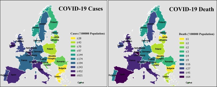
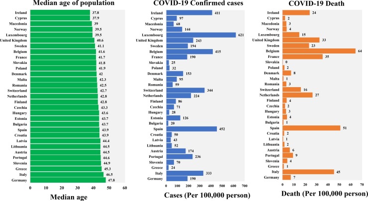
The spatial distribution of COVID-19 cases and deaths are presented in Fig. 1 . The highest number of cases (per 100,000 population) were observed in Luxembourg, Spain, Belgium, Ireland, Switzerland, Italy, etc. In comparison, comparably lower COVID-19 cases (per 100,000 people) were accounted in Bulgaria, Greece, Slovakia, Hungary, Poland, Latvia, Lithuania, respectively. In addition to this, moderate levels of COVID-19 cases (per 100,000 people) were counted for United Kingdom, Netherlands, Portugal, France, Sweden, and Austria (Fig. 1, Fig. 2 ). Considering the COVID-19 deaths (per 100,000 population) across Europe, the maximum counts were recorded in Belgium, Spain, Italy, France, United Kingdom, and moderate level morbidity was observed in Netherlands, Ireland, Sweden, Switzerland, Luxembourg, etc. Moreover, considerably lower COVID-19 deaths (per 100,000 population) were reported in Slovakia, Greece, Latvia, Malta, Croatia, Lithuania, Poland, Cyprus, Romania, Hungary, Slovenia, respectively (Fig. 1, Fig. 2). These heterogeneous distributions of COVID cases and deaths can be linked with the socio-demographic pattern of the country.

Fig. 1.

The spatial distribution of COVID-19 cases and deaths across Europe.

Fig. 2.

The distribution of median age of population, COVID case intensity, COVID death intensity in different European countries.

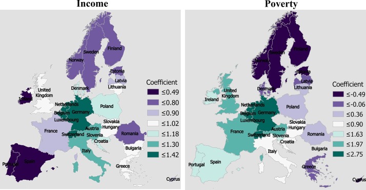
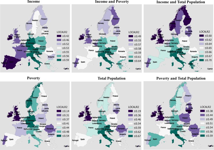
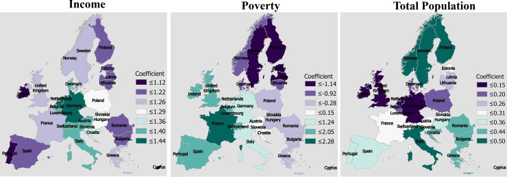
The spatially varying local R² and coefficient values for each explanatory variable were computed using the GWR model (Fig. 3, Fig. 4, Fig. 5, Fig. 6 , Table S2). These figures are collectively demonstrating the profound impact of socio-demographic components on overall COVID patterns in Europe. Considering local R² values for the cases, the highest association between socio-demographic variables and the COVID-19 cases was observed in Germany (R² = 0.93), Austria (R² = 0.93), Slovenia (R² = 0.92), Switzerland (R² = 0.92). The moderate local R² was observed for Italy (R² = 0.90), Luxembourg (R² = 0.90), Poland (R² = 0.90), Denmark R² = 0.89), Croatia (R² = 0.89), Belgium (R² = 0.87), Slovakia (R² = 0.87), and Netherlands (R² = 0.86). The lowest local R² value for COVID-19 cases was accounted for Ireland (R² = 0.56), Portugal (R² = 0.58), United Kingdom (R² = 0.66), and Spain (R² = 0.67) (Fig. 3). In addition to the Local R² approximation, the spatially varying coefficient values for the explanatory variables were also analyzed and presented in Fig. 4. For income factor, all the European countries exhibited a positive coefficient with different intensity, found highest in Germany, Belgium, Netherland, Italy, Austria, Slovenia, Switzerland. In contrast, comparably lower coefficient values have been approximated for Spain, Portugal, Ireland, Norway, Sweden, Finland (Fig. 4). On the other hand, a two-parameter GWR model, which has been developed for evaluating the association between poverty and COVID cases in the European countries, has produced a negative coefficient for many cases (Fig. 4). This indicates that poverty and COVID cases are negatively associated. For the COVID deaths, four-parameter regression models were developed using the local GWR model (Fig. 5 ). The highest association between the explanatory variables, i.e. poverty, income, total populations and COVID death was accounted for Italy (R² = 0.71), Croatia (R² = 0.68), Slovenia (R² = 0.67), Austria (R² = 0.65), Hungary (R² = 0.64), and Greece (R² = 0.64). Conversely, the minimum association between these variables and COVID deaths were found in United Kingdom (R² = 0.002), Ireland (R² = 0.07), Netherland (R² = 0.44), Cyprus (R² = 0.45), Lithuania (R² = 0.46), Latvia (R² = 0.48) (Fig. 5). In addition to the regression estimates, the spatially varying and autocorrelated coefficient estimates of the three explanatory variables were also measured and documented in Fig. 6. Among the three variables, income and total population have exhibited a positive coefficient in the regression modelling. As expected, a negative association between poverty and COVID deaths was found in Northern European region, especially in Norway, Finland, Sweden, Estonia, Latvia, Lithuania, respectively (Fig. 6).

Fig. 3.

The individual effect of the demographic variables on the COVID-19 case derived from the GWR model.

Fig. 4.

The spatial varying local regression coefficient estimated for the COVID case factor.

Fig. 5.

The individual effect of the demographic variables on COVID-19 death derived from the GWR model.

Fig. 6.

The spatial varying local regression coefficient estimated for the COVID death factor.

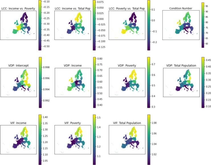
The spatial distribution of four confirmatory components, i.e., local correlation coefficient, local condition number, local variation decomposition proportions, and local variation inflation factors, were computed using python programming, and the same is presented in Fig. 7 . All these factors collectively indicate the robustness of the multi-parameters GWR model conceptualized for this research. The lower values of spatial LCC, condition number, VDP, and VIF are suggesting that the independent variables chosen for the modelling does not have multi-collinearity problems among the observation and have substantial explanatory power to explain maximum model variances. Additionally, for all three explanatory variables, a negligible spatial local correlation and VIF values were computed, which lies within the acceptable threshold (Fig. 7). Based on these unbiased explanatory variables, a set of multi-parameter local GWR models was performed. For COVID cases, the three-parameter regression model has explained 88 % model variances, and for COVID death, the four-parameter regression model was able to explain 70 % model variances (Table 1 ). Additionally, both models are statistically significant at P = 0.05 significance level.

Fig. 7.

Spatial distribution of local correlation coefficient, local condition number, local variation decomposition proportions, and variance inflation factors, estimated from local GWR model.

Table 1.

Overall explanatory statistics of the GWR model.

Factors	Response variable	R2	Adj.R2	Sigma2	Sigma2 MLE	AICc
VIFCase	Cases	0.88	0.83	0.1681	0.1200	40.21
VIFDeath	Death	0.72	0.60	0.7712	0.5584	82.23

The individual impact of the socio-demographic variables (2 for COVID-19 cases and 3 for COVID-19 death) on COVID incidences are also evaluated using both global (OLS) and local (GWR) regression model (Table 2, Table 3, Table 4 ). Among the 2 variables approximated for the COVID cases, the highest local R² was calculated for income (R² = 0.82), followed by poverty (R² = 0.74) (Table 2). However, the interaction effect of these variables was found much higher (R² = 0.85) than the individual effect. For COVID deaths, the total population factor exhibited the highest individual effect (R² = 0.68), followed by income (R² = 0.57), and poverty (R² = 0.55), respectively. All these values were found statistically significant at different probability levels. Considering the combined effect of these variables on COVID death, the interaction effect of income and total population was found highest (R² = 0.68), followed by income/poverty (R² = 0.62), and poverty/total population (R² = 0.62). Except for income/total population, the interaction effects of the other variables (income/poverty and poverty/total population) was found higher than their individual effect. The global OLS model was also performed to re-confirm the local modelling estimates, and the results of the same are presented in Table 3, Table 4. The three-parameter regression model approximated for the COVID cases has explained 76 % model variances, which was found much lower than the local GWR model (88 %). For the COVID deaths, the four parameters global OLS model has explained 68 % model variances, which is also way lower than the variances explained by local GWR model (72 %). Therefore, after taking examples from the explanatory power of both local and global regression models, it is recommended to adopt local regression models when the dependent or target variables are spatially inter-linked and auto-correlated. The PLS and PCR models were also executed for examining the model variances and to develop multivariate regression models for reproducibility and effective replication of the approaches adopted in this study. For cases, the PLS and PCR models have explained 68 % model variances, and for deaths, the PLS and PCR models have explained 63 % and 64 % model variances, which appears to be much lower than the variance explained by local GWR model (Table 5 ).

Table 2.

The association between the demographic variables and total COVID-19 cases across the Europe derived from GWR model. Inc - Income; Pov - Poverty, TotPop - Total Population.

Variable	Response variable	R2	Adj.R2	Sigma 2	Sigma2 MLE	AICc
Inc	Cases	0.82	0.74	0.26	0.18	53.44
Pov	Cases	0.74	0.59	0.39	0.26	67.74
Inc/Pov	Cases	0.85	0.80	0.20	0.15	43.54
Inc	Death	0.57	0.48	1.02	0.85	86.70
Pov	Death	0.55	0.39	1.19	0.88	93.87
TotPop	Death	0.68	0.56	0.85	0.60	86.45
Inc/Pov	Death	0.62	0.50	0.98	0.76	87.79
Inc/TotPop	Death	0.68	0.58	0.82	0.63	83.28
Pov/TotPop	Death	0.62	0.43	1.11	0.75	95.91

Table 3.

Ordinary Least Square model summary statistics and spatial dependence analysis. Inc - Income; Pov - Poverty; TotPop - Total Population.

Factor	Model	Value	t-Statistic	Probability
Cases	Constant	−13.73	−5.41	0.0000
	Inc	1.36	8.77	0.0000
	Pov	1.95	3.74	0.0010
	R2	0.76
	Adj.R2	0.74
	F	38.62
	P (F Test)	0.00
	AIC	45.53
Death	Constant	−26.45	−5.69	0.0000
	Inc	1.55	6.08	0.0000
	Pov	2.08	2.42	0.0236
	TotPop	0.48	3.81	0.0008
	R2	0.68
	Adj.R2	0.64
	F	17.35
	P (F Test)	0.00
	AIC	74.24
	Spatial Dependence	MI/DF	Value	Probability
Cases	Moran's I (error)	0.48	3.29	0.0010
	Lagrange Multiplier (lag)	1	4.97	0.0258
	Robust LM (lag)	1	1.44	0.2301
	Lagrange Multiplier (error)	1	7.07	0.0078
	Robust LM (error)	1	3.54	0.0598
	Lagrange Multiplier (SARMA)	2	8.51	0.0142
Death	Moran's I (error)	0.14	1.28	0.1999
	Lagrange Multiplier (lag)	1	3.59	0.0580
	Robust LM (lag)	1	3.94	0.0472
	Lagrange Multiplier (error)	1	0.59	0.4436
	Robust LM (error)	1	0.93	0.3345
	Lagrange Multiplier (SARMA)	2	4.53	0.1041

Table 4.

Ordinary Least Square model summary statistics for cases and death . Inc - Income; Pov - Poverty; TotPop - Total Population.

Criteria	Factor	Source	Value	Std.Error	t	Pr > |t|	Lower bound (95 %)	Upper bound (95 %)
Model Estimates	Cases	Intercept	−10.523	2.352	−4.474	0.000	−15.341	−5.705
		Inc	1.162	0.150	7.773	< 0.0001	0.856	1.468
		Pov	1.507	0.486	3.103	0.004	0.512	2.502
	Death	Intercept	−23.483	4.239	−5.540	< 0.0001	−32.180	−14.785
		TotPop	0.473	0.120	3.930	0.001	0.226	0.720
		Inc	1.308	0.239	5.464	< 0.0001	0.817	1.800
		Pov	1.883	0.779	2.417	0.023	0.284	3.481
Standardized Coefficients	Cases	Inc	0.916	0.118	7.773	< 0.0001	0.674	1.157
		Pov	0.365	0.118	3.103	0.004	0.124	0.607
	Death	TotPop	0.459	0.117	3.930	0.001	0.219	0.698
		Inc	0.703	0.129	5.464	< 0.0001	0.439	0.968
		Pov	0.312	0.129	2.417	0.023	0.047	0.576

Table 5.

PCR and PLS derived model estimates showing the strong association between demographic variables and COVID-19 spread and death in Europe. Inc - Income; Pov - Poverty; TotPop - Total Population.

Model	Factor	Model description	R2	MSE	RMSE
PCR	Cases	Cases = −10.52 + 1.16*Inc+1.51*Pov	0.68	0.317	0.563
	Death	Death = −23.48 + 0.47*TotPop+1.31*Inc+1.88*Pov	0.64	0.812	0.901
PLS	Cases	Cases = −10.52 + 1.16*Inc+1.51*Pov	0.68	0.286	0.535
	Death	Death = −23.16 + 0.53*TotPop+1.21*Inc+1.78*Pov	0.63	0.717	0.847

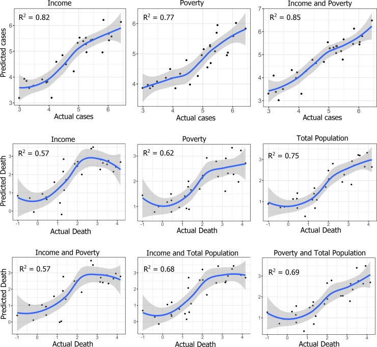
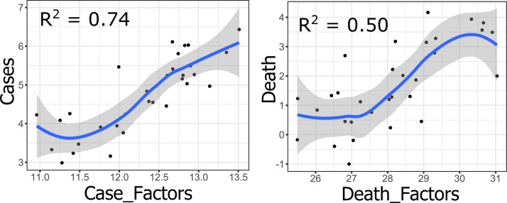
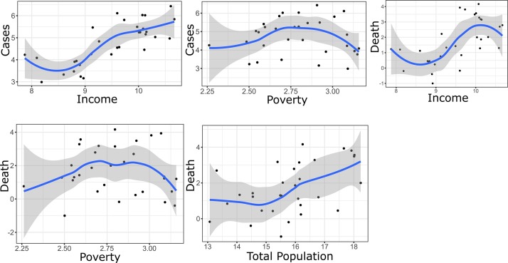
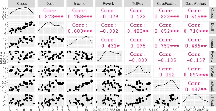
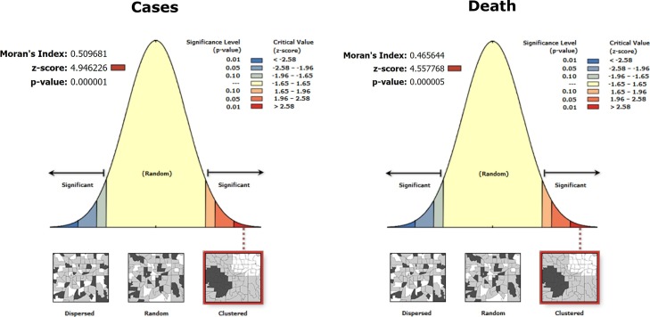
Using the multi-parameter regression models, the prediction of COVID-19 cases and deaths was made using the local GWR model (Fig. 8 ). For the cases, the income factor has predicted the COVID cases with 82 % accuracy. On the other hand, the prediction accuracy (77 %) was found much lower for the poverty factor. Combinedly, poverty and income factors have explained substantial model variances and predicted the COVID cases with 85 % accuracy. For the deaths, the predictive power of all three explanatory variables was measured and found highest for the total population (75 %), followed by poverty (62 %) and income (57 %). Therefore, the GWR based prediction for both cases and deaths is suggesting the superiority of spatial regression models in explaining the heterogeneous distribution of COVID cases and deaths across Europe. Additionally, spatial regression modelling will be highly effective, where spatial dependence among the observation is quite obvious and omnipresent. Fig. 9, Fig. 10 shows the linear association between socio-demographic variables and COVID-19 for different parametric models. For the COVID-19 cases, the coefficient of determination (R²) value was recorded as 0.74, while for the deaths, the linear model has explained 50 % model variances (Fig. 9). Fig. 10 explained the linear association between each socio-demographic variables and COVID-19 cases and death. Among the three socio-demographic variables, the income and total population factors exhibited a strong association with COVID cases/deaths. In comparison, the poverty factor has not shown any strong association with COVID cases/deaths. The correlation among and between the socio-demographic variables and COVID-19 cases and deaths are presented in Fig. 11 . Among the driving factors, a high correlation was observed for income; a comparably weak association was accounted for the total population factor. Moreover, a weak negative correlation was found between poverty and COVID factors (Fig. 11). In addition to this, the correlation between the case and death factors (all the three explanatory variables approximated for cases/deaths were merged together for evaluating their collective influence on COVID cases) and COVID counts was found higher than their individual impact. The spatial dependency among the observation was tested using global Moran’s I statistics (Fig. 12 ). For both cases and deaths, a statistically significant spatial cluster was found. The Local Moran’s I have produced a similar pattern, where 4 European countries are exhibiting a high-high spatial cluster, 3 countries show low-low spatial cluster, and a high-low spatial cluster was observed for a single country (Fig. S1). The spatial cluster and outliers were measured for the explanatory variables using the Local Geary C multivariate cluster method, and the same is presented in Fig. S1. A total of 6 statistically significant spatial clusters was calculated, among which 4 were significant at P = 0.05 significance level, and 2 clusters were found significant at P = 0.01 significance level. For evaluating the robustness and accuracy of the spatial regression models, the normality check was done for standardized residuals of the GWR model, and for all explanatory variables, statistically significant normality scores were measured, which combinedly suggesting that model estimates are not biased and irrelevant.

Fig. 8.

The predicted values of COVID-19 case and death derived from the GWR model.

Fig. 9.

The linear association between socio-demographic components and COVID case/death counts.

Fig. 10.

The linear association between 3 socio-demographic variables and COVID-19 case/death.

Fig. 11.

The correlation between the selected socio-demographic variables and COVID-19 case/death. TotPop - total population.

Fig. 12.

Global Moran's I spatial dependency test for evaluating the statistical significance of spatial clusters of the distribution.

The overall summary of the four spatial regression models is reported in Table 6. Among the 2 socio-demographic variables chosen for the cases, the average R² was observed for income (R² = 0.71), followed by poverty (R² = 0.45), respectively. For deaths, the highest R² value was calculated for income (R² = 0.51), followed by total population (R² = 0.49), and poverty (R² = 0.39), respectively. Considering the results of all four spatial regression models, the socio-demographic variables explained 88 % model variances for the COVID-19 cases and 72 % model variances for the COVID-19 deaths (Table 1).

Table 6.

Overall summary of spatial regression models that indicates the linkages between the socio-demographic variables and total COVID-19 cases and deaths across Europe. Inc - Income; Pov - Poverty; TotPop - Total Population

			Spatial Regression Models
			Global			Local
Factor	Variable	Parameter	SEM	SLM	OLS	GWR	Average
Cases	Inc	R2	0.72	0.67	0.62	0.82	0.71
		AIC	50.44	54.38	55.97	53.44	53.56
		SIC	53.10	58.38	58.63	-----	56.71
	Pov	R2	0.70	0.34	0.00	0.74	0.45
		AIC	58.42	75.24	82.90	67.74	71.07
		SIC	61.08	79.23	85.56	-----	75.29
Death	Inc	R2	0.49	0.56	0.42	0.57	0.51
		AIC	84.72	83.35	87.14	86.70	85.48
		SIC	87.38	87.35	89.80	----	88.18
	Pov	R2	0.52	0.49	0.01	0.55	0.39
		AIC	88.05	90.91	102.36	93.87	93.80
		SIC	90.71	94.91	105.03	----	96.88
	TotPop	R2	0.53	0.54	0.19	0.70	0.49
		AIC	86.03	86.88	96.50	86.45	88.96
		SIC	88.69	90.87	99.17	----	92.91

4. Discussion

The spatial distribution of COVID-19 deaths and confirmed cases were examined in order to understand how the socio-demographic structure of a country can regulate the overall casualties caused by the novel coronavirus. The distribution of the COVID-19 confirmed cases and deaths were found heterogeneous across Europe. This uneven distribution could be attributed to many corresponding factors, including demography, climatic, cultural, or socio-economic differences among the countries. For both COVID-19 cases and deaths, the maximum records (actual values) were documented in the western European region (Spain, Italy, France, Germany, UK, Belgium, Netherlands). While, the cases and deaths were found lower (actual values) in the Eastern (Romania, Bulgaria, Greece, Estonia, Latvia, Lithuania) and Northern European region (Norway, Finland, Sweden). However, the above pattern is found somewhat different when the proportion or density of COVID cases and deaths were taken into consideration. For instance, the case density (cases per 100 000 persons) was found maximum in Luxembourg, Belgium, Spain, Ireland, and found minimum in Bulgaria, Greece, Slovakia. These statistical figures suggest that the rate of COVID infection, which indeed portray more logical and reliable estimates than its absolute counterparts, should be taken into account for unbiased estimation and effective interpretation of results. Additionally, the uneven distribution (for both cases and deaths of COVID-19) in the European countries could be linked to the age of the population (old age and median age of population). It can be seen in Fig. 2, the median age of population in Italy and Spain is 46.5 and 43.9, and these two countries affected badly by COVID pandemic in terms of the number of cases and deaths. As of 11th July 2020, total 34,938 and 28,403 deaths were recorded so far in Italy and Spain10 . The spatial association between the socio-demographic variables and COVID-19 cases and deaths were found maximum in the central European regions (Germany, Switzerland, Italy, Austria). All these countries have been affected badly in terms of the total number of cases and deaths caused by COVID-19. For the cases, a weak association between income and the COVID-19 cases was evident in the western European countries (Portugal, Spain, Ireland). The same association was found considerably high in the central European region. This suggests that income factors do not have a uniform and spatial stationary interaction with COVID cases. Several factors could be responsible for this uneven distribution of spatial association. This includes the age structure of the population, ratio of the elderly population, ratio of dependent population, pre-existing health records, human mobility, the socio-economic structure of the society, etc. The intercept values were calculated for the two response variables (cases and deaths), which followed the same pattern as observed for the regression estimates. The individual influences of all the socio-demographic variables on COVID-19 cases and deaths were analysed, and these variables have exhibited a statistically significant spatially dependent model estimates.

Using all the (non)spatial regression models including GWR, OLS, SLM, SER, PCR, PLS, MLR, the individual and interaction effect of the demographic variables on COVID-19 cases and deaths were analyzed and reported. Among the 2 variables considered for COVID-19 cases, the income factor has strongly regulated the COVID-19 cases across the European region. For the COVID deaths, the income and total population factors were strongly correlated with the deaths and explained substantial model variances. The positive association between income/total population and COVID cases/deaths indicates that these two factors could be the key controlling variables that determine the overall casualties caused by this pandemic in the European countries. A similar close association between the socio-demographic factors and COVID-19 was observed in Wuhan, China (Wu, Chen, Cai et al., 2020). Wu, Chen, Cai et al. (2020) found a close association between pre-existing illness of the patients, including Acute Respiratory Distress Syndrome (ARDS) and Pneumonia and its association with COVID-19 and stated that patients with existing respiratory illness were more susceptible to COVID-19. The psychological status of the people, especially the old age people, is closely linked with the diagnostic of COVID 19 (Wang et al., 2020). Therefore, the combination of effective psychological interventions, including the lower level of psychological pressure and behavioural practices that boost mental health, can be used to improve the psychological status of vulnerable communities (Wang et al., 2020). Aging adults (>65) with long-term illness and incapable of household works were found highly vulnerable COVID-19 (Lakhani, 2020). The proportion of deaths due to COVID-19 in Italy, Netherlands, Spain, and France was 50 %, 58 %, 59 %, and 59 % for the population with age >80 (Medfod & Trias-Llimos, 2020). (Likassa, 2020), stated that the spatial distribution of COVID-19 cases was highly associated with case-fatality rate, and the linkages between these two variables were much stronger and reached up to 8.0 % for patients with the age group of 70–79 years and 14.8 % for patients aged >80 years. Likassa (2020) also stated that the high infection and death rate in China, Italy, Iran, and the USA, could be linked with the spread of previous virus outbreak. Lippi, Mattiuzzi, Sanchis-Gomar and Henry (2020) stated that three main determinants – male sex, population with age >60, and pre-existing comorbidities such as diabetes, hypertension, chronic respiratory diseases, cancer, and cardiovascular disorders, strongly determine the rate of COVID-19 death and infection. These statistics signifying the inherent connections amongst the socio-demographic composition and overall COVID-19 deaths and cases reported so far in the European region (Almagro & Orane-hutchinson, 2020; Borjas, 2020; Dowd et al., 2020; Jia et al., 2020; Mollalo et al., 2020). Apart from the demographic factors, several climatic factors, including average temperature, minimum temperature, maximum temperature, rainfall, average humidity, wind speed, and air quality has also regulated the spread and casualties of COVID-19 (Bashir et al., 2020; Ma et al., 2020). The availability of sufficient SARS-CoV-2 testing centers is also found to be important for adopting control strategies and decision making for minimizing the impact of COVID-19 on the overall socio-ecological system (Rader et al., 2020). In addition to this, Kraemer et al. (2020) found that human mobility factors is the key critical factor that aggravated the spread of COVID-19 cases in China as the growth rates become stable or negative in some areas where strong control measures were implemented and mandatorily imposed. However, the mobility factors in the other regions where the stringent regulations were not implemented, still pose severe threats by transmitting the infection in the closest neighbours (Kraemer et al., 2020). Therefore, it has been suggested that paying more attention to controlling (inter)national migration, restricted population flows, modernizing the healthcare system by improving diagnosis and treatment capacity, and upgrading the public welfare system to make it fully functional for the crisis situation, could be the point of interest in order to fight against the COVID-19 like situation effectively (Su et al., 2020).

Cities in the developing and developed world, including the UNESCO defined creative cities, which was designed in 2004 for providing maximum priority on creativity and sustainable urban development by achieving efficiency in all aspects, have been impacted badly by the outbreak of COVID pandemic. Though the long-term impact of COVID-19 on urban and city environment is challenging to predict, the historical shreds of evidence suggest that the long-term inelastic and old fashioned exhausted strategical plans of cities had always been shaped by strong interventions, like the outbreak of deadly viral diseases, natural calamities such as flood or earthquake11 . Therefore, it is highly expected that in COVID-19 recovery period, the concerned stakeholders, including governments bodies, decision-makers, businesses leaders, city planners, land administrators, etc. will be directed in a way that forced them to re-think the viability of existing plans and find more comprehensive solutions that accelerate sustainability in city planning. There are few specific areas where complete structural reforms can be done, such as promoting a healthier building environment, which characterized by clean indoor air quality for both office and home environment. Healthier indoor environments can enhance the cognitive performance of a person that eventually boosts the logical and emotional intelligence of the person. Therefore, more focus on nature-based landscape design, such as open spaces and greenery for meditation, exercise, green material in living areas, proper ventilation system, uses of energy-efficient building materials, will be the need of the day.

5. Conclusion

In this study, the spatial association between the socio-demographic variables and COVID-19 cases and deaths was evaluated across Europe. The distribution of the COVID-19 confirmed cases and deaths were found heterogeneous across Europe. This uneven distribution could be attributed to many corresponding factors, including demography, climatic, cultural, or socio-economic differences among the countries. For both COVID-19 cases and deaths, the maximum records (actual values) were documented in the western European region (Spain, Italy, France, Germany, UK, Belgium, Netherlands). While, the cases and deaths were found lower (actual values) in the Eastern (Romania, Bulgaria, Greece, Estonia, Latvia, Lithuania) and Northern European region (Norway, Finland, Sweden). This can be attributed to the socio-demographic composition of these countries as Italy has the second oldest population (23 %) in the world and the oldest in Europe (population ages 65 and above). The population composition of the other European countries, i.e., Spain, France, and the Netherlands, that affected badly by COVID-19, is also dominated by senior and old age populations, thereby increasing the vulnerability to COVID-19 and many similar COVID-19 pandemics in the future. The case density (cases per 100, 000 persons) was found maximum in Luxembourg, Belgium, Spain, Ireland, and found minimum in Bulgaria, Greece, Slovakia. In comparison, the death intensity is highest in Belgium, Spain, Italy, and the lowest in Slovakia, Bulgaria, Greece, respectively. These statistical figures suggest that the rate of COVID infection and rate of COVID recovery, which indeed portrays a more logical and reliable estimate than its absolute counterparts, should be taken into account for unbiased estimation and effective interpretation of results. To explain this spatial non-stationary distribution of COVID cases/death and to examine the spatial dependency among the observation, several spatial regression models, including GWR, OLS, SLM, SEM, etc. was performed. COVID cases and death counts were considered as dependent variables for regression modelling. All the explanatory variables produced a statistically significant locally varying associations with COVID cases/death. The highest association was accounted for Germany, Austria, Italy, Spain, Luxembourg, Croatia. A strong positive association between income/total population and COVID cases/deaths is found in this study, which indicates that these two factors could be the key controlling variables that determine the overall casualties caused by COVID-19 European countries. In this study, the influence of the other controlling factors such as environmental pollution, socio-ecological status, climatic extremity, etc. have not been considered. This could be scope for future research.

CRediT authorship contribution statement

Srikanta Sannigrahi: Conceptualization, Data curation, Formal analysis, Writing - review & editing. Francesco Pilla: Conceptualization, Supervision, Writing - review & editing. Bidroha Basu: Conceptualization, Supervision, Writing - review & editing. Arunima Sarkar Basu: Conceptualization, Writing - review & editing. Anna Molter: Conceptualization, Writing - review & editing.

Declaration of Competing Interest

The authors whose names are listed in this manuscript certify that they have NO conflict of interest for subject matter or materials discussed in this manuscript.

Appendix A. Supplementary data

The following are Supplementary data to this article:

References

- Almagro M., Orane-hutchinson A. 2020. The determinants of the differential exposure to COVID-19 in New York City and their evolution over time. [DOI] [PMC free article] [PubMed] [Google Scholar]
- Anselin L. Spatial externalities, spatial multipliers and spatial econometrics. International Regional Science Review. 2003;26(2):153–166. [Google Scholar]
- Anselin L., Arribas-Bel D. Spatial fixed effects and spatial dependence in a single cross-section. Papers in Regional. 2013;92(1):3–17. [Google Scholar]
- Bashir M.F., Ma B., Bilal, Komal B., Bashir M.A., Tan D., Bashir M. Correlation between climate indicators and COVID-19 pandemic in New York, USA. The Science of the Total Environment. 2020;728 doi: 10.1016/j.scitotenv.2020.138835. [DOI] [PMC free article] [PubMed] [Google Scholar]
- Blyth M.J.G., Kincaid R., Craigen M.A.C., Bennet G.C. The changing epidemiology of acute and subacute haematogenous osteomyelitis in children. The Journal of Bone and Joint Surgery British Volume. 2001;83(1):99–102. doi: 10.1302/0301-620x.83b1.10699. [DOI] [PubMed] [Google Scholar]
- Borjas G.J. Demographic determinants of testing incidence and COVID-19 infections in New York City neighborhoods. SSRN Electronic Journal. 2020 doi: 10.2139/ssrn.3572329. [DOI] [Google Scholar]
- Brunsdon C., Fotheringham A.S., Charlton M.E. Geographically weighted regression: A method for exploring spatial nonstationarity. Geographical Analysis. 1996;28(4):281–298. doi: 10.1111/j.1538-4632.1996.tb00936.x. [DOI] [Google Scholar]
- Brunsdon C., Fotheringham A.S., Charlton M. Geographically weighted summary statistics—A framework for localised exploratory data analysis. Computers, Environment and Urban Systems. 2002;26(6):501–524. [Google Scholar]
- Chakraborti S., Banerjee A., Sannigrahi S., Pramanik S., Maiti A., Jha S. Assessing the dynamic relationship among land use pattern and land surface temperature: A spatial regression approach. Asian Geographer. 2019;36(2):93–116. [Google Scholar]
- Chen W., Shen Y., Wang Y. Does industrial land price lead to industrial diffusion in China? An empirical study from a spatial perspective. Sustainable Cities and Society. 2018;40:307–316. [Google Scholar]
- Chi G., Zhu J. Spatial regression models for demographic analysis. Population Research and Policy Review. 2008;27(1):17–42. doi: 10.1007/s11113-007-9051-8. [DOI] [Google Scholar]
- Congessional Research Service . 2020. Global econoic effects of COVID-19.https://fas.org/sgp/crs/row/R46270.pdf Retrieved from. [Google Scholar]
- Diuk-Wasser M.A., Brown H.E., Andreadis T.G., Fish D. Modeling the spatial distribution of mosquito vectors for West Nile Virus in Connecticut, USA. Vector-Borne and Zoonotic Diseases. 2006;6(3):283–295. doi: 10.1089/vbz.2006.6.283. [DOI] [PubMed] [Google Scholar]
- Dowd J.B., Andriano L., Brazel D.M., Rotondi V., Block P., Ding X.…Mills M.C. Demographic science aids in understanding the spread and fatality rates of COVID-19. Proceedings of the National Academy of Sciences. 2020 doi: 10.1073/pnas.2004911117. [DOI] [PMC free article] [PubMed] [Google Scholar]
- Duan L., Zhu G. Psychological interventions for people affected by the COVID-19 epidemic. The Lancet Psychiatry. 2020;7(4):300–302. doi: 10.1016/S2215-0366(20)30073-0. [DOI] [PMC free article] [PubMed] [Google Scholar]
- Fang C., Liu H., Li G., Sun D., Miao Z. Estimating the impact of urbanization on air quality in China using spatial regression models. Sustainability (Switzerland) 2015;7(11):15570–15592. doi: 10.3390/su71115570. [DOI] [Google Scholar]
- Fotheringham A., Charlton M., Brunsdon C. The geography of parameter space: An investigation of spatial non-stationarity. International Journal of Geographical Information Systems. 1996;10(5):605–627. [Google Scholar]
- Fotheringham A.S., Oshan T.M., (2016) Geographically weighted regression and multicollinearity: dispelling the myth. Journal of Geographical Systems. 2016;18(4):303–329. [Google Scholar]
- Fu L., Fei J., Xiang H.-X., Xiang Y., Tan Z.-X., Li M.-D., Xu D.-X. Analysis of death risk factors among 200 COVID-19 patients in Wuhan, China: A hospital-based case-cohort study. SSRN Electronic Journal. 2020;86(551) doi: 10.2139/ssrn.3551430. [DOI] [Google Scholar]
- Goodchild M.F., Parks B.O., Steyaert L.T. 1993. Environmental modeling with GIS. [Google Scholar]
- Gorbalenya A.E., Baker S.C., Baric R.S., Groot R.J.D., Gulyaeva A.A., Haagmans B.L., Leontovich A.M. The species and its viruses – A statement of the coronavirus study group. Biorxiv (Cold Spring Harbor Laboratory) 2020:1–15. doi: 10.1101/2020.02.07.937862. [DOI] [Google Scholar]
- Guo A., Yang J., Xiao X., Xia J., Jin C., Li X. Influences of urban spatial form on urban heat island effects at the community level in China. Sustainable Cities and Society. 2020;53 [Google Scholar]
- Guo G., Wu Z., Chen Y. Evaluation of spatially heterogeneous driving forces of the urban heat environment based on a regression tree model. Sustainable Cities and Society. 2020;54 [Google Scholar]
- Jain S., Sannigrahi S., Sen S., Bhatt S., Chakraborti S., Rahmat S. Urban heat island intensity and its mitigation strategies in the fast-growing urban area. Journal of Urban Management. 2019;9(October 2019):5856. doi: 10.1016/j.jum.2019.09.004. [DOI] [Google Scholar]
- Jia J.S., Lu X., Yuan Y., Xu G., Jia J., Christakis N.A. Population flow drives spatio-temporal distribution of COVID-19 in China. Nature. 2020:1–11. doi: 10.1038/s41586-020-2284-y. [DOI] [PubMed] [Google Scholar]
- Kauhl B., Heil J., Hoebe C.J.P.A., Schweikart J., Krafft T., Dukers-Muijrers N.H.T.M. The spatial distribution of hepatitis C virus infections and associated determinants--An application of a geographically weighted poisson regression for evidence-based screening interventions in hotspots. PloS One. 2015;10(9):e0135656. doi: 10.1371/journal.pone.0135656. [DOI] [PMC free article] [PubMed] [Google Scholar]
- Kraemer M.U.G., Yang C.H., Gutierrez B., Wu C.H., Klein B., Pigott D.M.…Scarpino S.V. The effect of human mobility and control measures on the COVID-19 epidemic in China. Science (New York, NY) 2020;497(May):493–497. doi: 10.1126/science.abb4218. [DOI] [PMC free article] [PubMed] [Google Scholar]
- Kulu H., Dorey P. The contribution of age structure to the number of deaths from Covid-19 in the UK by geographical units. MedRxiv. 2020 doi: 10.1101/2020.04.16.20067991. 2020.04.16.20067991. [DOI] [Google Scholar]
- Lakhani A. Which Melbourne metropolitan areas are vulnerable to COVID-19 based on age, disability and access to health services? Using spatial analysis to identify service gaps and inform delivery. Journal of Pain and Symptom Management. 2020 doi: 10.1016/j.jpainsymman.2020.03.041. [DOI] [PMC free article] [PubMed] [Google Scholar]
- Lewis F.I., Ward M.P. Improving epidemiologic data analyses through multivariate regression modelling. Emerging Themes in Epidemiology. 2013;10(1):1–10. doi: 10.1186/1742-7622-10-4. [DOI] [PMC free article] [PubMed] [Google Scholar]
- Linard C., Lamarque P., Heyman P., Ducoffre G., Luyasu V., Tersago K.…Lambin E.F. Determinants of the geographic distribution of Puumala virus and Lyme borreliosis infections in Belgium. International Journal of Health Geographics. 2007;6(1):15. doi: 10.1186/1476-072X-6-15. [DOI] [PMC free article] [PubMed] [Google Scholar]
- Lippi G., Mattiuzzi C., Sanchis-Gomar F., Henry B.M. Clinical and demographic characteristics of patients dying from COVID-19 in Italy versus China. Journal of Medical Virology. 2020:0–3. doi: 10.1002/jmv.25860. [DOI] [PMC free article] [PubMed] [Google Scholar]
- Likassa H.T., 2020 The Impacts of Covariates on Spatial Distribution of CORONA Virus 2019 (COVID-19): WHO Data through Multivariate Analysis of Covariance (MANCOVA). Eurasian J. Med. Oncol . 2020;4:141–148. doi: 10.14744/ejmo.2019.81104. [DOI] [Google Scholar]
- Liu X., Sun T., Feng Q. Dynamic spatial spillover effect of urbanization on environmental pollution in China considering the inertia characteristics of environmental pollution. Sustainable Cities and Society. 2020;53 [Google Scholar]
- Liu Y., Zhang Y., Jin S.T., Liu Y. Spatial pattern of leisure activities among residents in Beijing, China: Exploring the impacts of urban environment. Sustainable Cities and Society. 2020;52 [Google Scholar]
- Lugoi L.P., Bamutaze Y., Martinsen V., Dick Ø.B., Almås Å.R. Ecosystem productivity response to environmental forcing, prospect for improved rain-fed cropping productivity in Lake Kyoga Basin. Applied Geography. 2019;102(September 2018):1–11. doi: 10.1016/j.apgeog.2018.11.001. [DOI] [Google Scholar]
- Ma Y., Zhao Y., Liu J., He X., Wang B., Fu S.…Luo B. Effects of temperature variation and humidity on the death of COVID-19 in Wuhan, China. The Science of the Total Environment. 2020;724 doi: 10.1016/j.scitotenv.2020.138226. [DOI] [PMC free article] [PubMed] [Google Scholar]
- Malesios C., Chatzipanagiotou M., Demiris N., Kantartzis A., Chatzilazarou G., Chatzinikolaou S., Kostoulas P. A quantitative analysis of the spatial and temporal evolution patterns of the bluetongue virus outbreak in the island of Lesvos, Greece, in 2014. Transboundary and Emerging Diseases. 2020 doi: 10.1111/tbed.13553. n/a(n/a) [DOI] [PubMed] [Google Scholar]
- Medfod A., Trias-Llimos S. Population age structure only partially explains the large number of COVID-19 deaths at the oldest ages. MedRxiv. 2020 doi: 10.1101/2020.04.09.20056341. 2020.04.09.20056341. [DOI] [Google Scholar]
- Meigs J.B. Invited commentary: Insulin resistance syndrome? Syndrome X? Multiple metabolic syndrome? A syndrome at all? Factor analysis reveals patterns in the fabric of correlated metabolic risk factors. American Journal of Epidemiology. 2000;152(10):908–911. doi: 10.1093/aje/152.10.908. [DOI] [PubMed] [Google Scholar]
- Merlo J., Chaix B., Ohlsson H., Beckman A., Johnell K., Hjerpe P.…Larsen K. A brief conceptual tutorial of multilevel analysis in social epidemiology: Using measures of clustering in multilevel logistic regression to investigate contextual phenomena. Journal of Epidemiology and Community Health. 2006;60(4):290–297. doi: 10.1136/jech.2004.029454. [DOI] [PMC free article] [PubMed] [Google Scholar]
- Mogi R., Spijker J. 2020. The influence of social and economic ties to the spread of COVID-19 in Europe; pp. 1–27. [DOI] [PMC free article] [PubMed] [Google Scholar]
- Mollalo A., Vahedi B., Rivera K.M. GIS-based spatial modeling of COVID-19 incidence rate in the continental United States. The Science of the Total Environment. 2020;728 doi: 10.1016/j.scitotenv.2020.138884. [DOI] [PMC free article] [PubMed] [Google Scholar]
- Oshan T.M., Li Z., Kang W., Wolf L.J., Stewart Fotheringham A. MGWR: A python implementation of multiscale geographically weighted regression for investigating process spatial heterogeneity and scale. ISPRS International Journal of Geo-information. 2019;8(6) doi: 10.3390/ijgi8060269. [DOI] [Google Scholar]
- Population Europe, 2020. https://population-europe.eu/news/demography-coronavirus.
- Rader B., Astley C.M., Sy K.T.L., Sewalk K., Hswen Y., Brownstein J.S., Kraemer M.U. Increased travel times to United States SARS-CoV-2 testing sites: A spatial modeling study. medRxiv. 2020 doi: 10.1093/jtm/taaa076. [DOI] [PMC free article] [PubMed] [Google Scholar]
- S. Sannigrahi, Q. Zhang, P.K. Joshi, P.C. Sutton, S. Keesstra, P.S. Roy, F. Pilla, B. Basu, Y. Wang, S. Jha and S.K. Paul, 2020. Examining effects of climate change and land use dynamic on biophysical and economic values of ecosystem services of a natural reserve region. Journal of Cleaner Production, 257, p.120424.
- Sannigrahi S., Zhang Q., Pilla F., Joshi P.K., Basu B., Keesstra S.…Chakraborti S. Responses of ecosystem services to natural and anthropogenic forcings: A spatial regression based assessment in the world’s largest mangrove ecosystem. The Science of the Total Environment. 2020;715 doi: 10.1016/j.scitotenv.2020.137004. [DOI] [PubMed] [Google Scholar]
- Slate, 2020. https://slate.com/news-and-politics/2020/04/graying-populations-economic-recovery.html.
- Su D., Chen Y., He K., Zhang T., Tan M., Zhang Y., Zhang X. Influence of socio-ecological factors on COVID-19 risk: A cross-sectional study based on 178 countries/regions worldwide. medRxiv. 2020 [Google Scholar]
- Sun Y., Wang S., Wang Y. Estimating local-scale urban heat island intensity using nighttime light satellite imageries. Sustainable Cities and Society. 2020 [Google Scholar]
- United Nations, 2020. https://www.un.org/en/.
- United Nations Department of Economic and Social Welfare, 2020. https://www.un.org/en/development/desa/population/migration/data/estimates2/estimates19.asp.
- Varraso R., Garcia-Aymerich J., Monier F., Le Moual N., De Batlle J., Miranda G.…Maccario J. Assessment of dietary patterns in nutritional epidemiology: Principal component analysis compared with confirmatory factor analysis. The American Journal of Clinical Nutrition. 2012;96(5):1079–1092. doi: 10.3945/ajcn.112.038109. [DOI] [PubMed] [Google Scholar]
- Wang C., Pan R., Wan X., Tan Y., Xu L., Ho C.S., Ho R.C. Immediate psychological responses and associated factors during the initial stage of the 2019 coronavirus disease (COVID-19) epidemic among the general population in China. International Journal of Environmental Research and Public Health. 2020;17(5) doi: 10.3390/ijerph17051729. [DOI] [PMC free article] [PubMed] [Google Scholar]
- Ward M.D., Gleditsch K.S. Vol. 155. Sage Publications; 2018. (Spatial regression models). [Google Scholar]
- World Health Organization, 2020. https://covid19.who.int/.
- Wu C., Chen X., Cai Y., Xia J., Zhou X., Xu S.…Song Y. Risk factors associated with acute respiratory distress syndrome and death in patients with coronavirus disease 2019 pneumonia in Wuhan, China. JAMA Internal Medicine. 2020:1–10. doi: 10.1001/jamainternmed.2020.0994. [DOI] [PMC free article] [PubMed] [Google Scholar]
- Wu Z., Chen Y., Han Y., Ke T., Liu Y. Identifying the influencing factors controlling the spatial variation of heavy metals in suburban soil using spatial regression models. The Science of the Total Environment. 2020;717 doi: 10.1016/j.scitotenv.2020.137212. [DOI] [PubMed] [Google Scholar]
- Yang X., Jin W. GIS-based spatial regression and prediction of water quality in river networks: A case study in Iowa. Journal of Environmental Management. 2010;91(10):1943–1951. doi: 10.1016/j.jenvman.2010.04.011. [DOI] [PubMed] [Google Scholar]
- Zhao R., Zhan L., Yao M., Yang L. A geographically weighted regression model augmented by Geodetector analysis and principal component analysis for the spatial distribution of PM2. 5. Sustainable Cities and Society. 2020;56 [Google Scholar]
- Zhou F., Yu T., Du R., Fan G., Liu Y., Liu Z.…Cao B. Clinical course and risk factors for mortality of adult inpatients with COVID-19 in Wuhan, China: A retrospective cohort study. Lancet. 2020;395(10229):1054–1062. doi: 10.1016/S0140-6736(20)30566-3. [DOI] [PMC free article] [PubMed] [Google Scholar]
Associated Data
This section collects any data citations, data availability statements, or supplementary materials included in this article.