Responses of Tropical Ocean Clouds and Precipitation to the Large-Scale Circulation:Atmospheric-Water-Budget-Related Phase Space and Dynamical Regimes

Abstract

An atmospheric-water-budget-related phase space is constructed with the tendency terms related to dynamical convergence (QCON ≡ −Q∇ · V) and moisture advection (QADV ≡ −V · ∇Q) in the water budget equation. Over the tropical oceans, QCON accounts for large-scale dynamical conditions related to conditional instability, and QADV accounts for conditions related to lower-tropospheric moisture gradient. Two reanalysis products [MERRA and ERA-Interim (ERAi)] are used to calculate QCON and QADV. Using the phase space as a reference frame, the Moderate Resolution Imaging Spectroradiometer (MODIS) cloud-top pressure (CTP) and cloud optical depth (COD) are used to evaluate simulated clouds in the GISS-E2 general circulation model. In regimes of divergence over the tropical oceans, moist advection yields frequent high- to midlevel medium-thickness to thick clouds associated with moderate stratiform precipitation, while dry advection yields low-level thin clouds associated with shallow convection with lowered cloud tops. In regimes with convergence, moist and dry advection modulate the relative abundance of high-level thick clouds and low-level thin to medium-thickness clouds. GISS-E2 qualitatively reproduces the cloud property dependence on moisture budget tendencies in regimes of convergence but with larger COD compared to MODIS. Low-level thick clouds in GISS-E2 are the most frequent in regimes of near-zero convergence and moist advection instead of those of large-scale divergence. Compared to the Global Precipitation Climatology Project product, MERRA, ERAi, and GISS-E2 have more rain in regimes with deep convection and less rain in regimes with shallow convection.

1. Introduction

Cloud feedbacks involving changes in the large-scale circulation have long been recognized as the main source of uncertainties in climate model projections of climate change caused by increases in greenhouse gases (Bony et al. 2015; Colman 2003; Dessler 2010; Randall et al. 2007; Ringer et al. 2006; Soden and Held 2006; Webb et al. 2006; Zelinka et al. 2012). Bony et al. (2015) state that understanding the interaction between clouds and circulation is urgently needed to accelerate progress in resolving discrepancies in climate sensitivity among models.

Previous process-oriented climate model evaluations have attempted to link climate variables (e.g., cloud amount) to large-scale dynamical conditions mainly through dynamical convergence (e.g., Bony and Dufresne 2005; Teixeira et al. 2011; Su et al. 2011, 2013) by using variables such as vertical velocity at 500 hPa, lower-tropospheric stability, and sea surface temperature. Bony et al. (2013) apply the atmospheric water budget equation to study climate change caused by CO₂ increase, but the work is mainly focused on the convergence (or vertical velocity) portion of the equation. Effects of horizontal moisture advection, which is important in areas with strong trade winds or tropical waves, are not explicitly investigated in these studies. In fact, the atmospheric water budget equation includes individual terms that are related to large-scale convergence and moisture advection and can be used to construct a thorough picture for water-budget-related large-scale dynamical conditions.

In section 2, we first define a phase space connecting large-scale dynamical conditions to metrics of the largescale atmospheric water budget. We further demonstrate the application of this phase space as a reference frame to represent large-scale dynamical conditions related to the varying combinations of effects of large-scale convergence (QCON) and moist advection (QADV). In section 3, we apply the water-budget-related phase space for climate model evaluation by studying simulated relationships among large-scale atmospheric water budgets, cloud properties, and precipitation in a free-running AGCM, the Goddard Institute for Space Studies Model E2 [GISS-E2; refer to Schmidt et al. (2014), with modifications described by Del Genio et al. (2012)]. Stratifying climate variables on the phase space provides a means to analyze how key climate variables (e.g., cloud properties) are related to large-scale dynamical conditions and the atmospheric water budget (e.g., precipitation). We focus on our study over the tropical oceans (30°S–30°N) to see whether this framework produces new insights as well as reproducing previous findings. Section 4 concludes our main results.

2. The water-budget-related phase space

a. Water vapor tendencies related to QCON and QADV

We define a phase space spanned by advection and convergence terms in the atmospheric water vapor budget equation (e.g., Peixoto and Oort 1992; Trenberth and Guillemot 1998; Wong et al. 2011; Bony et al. 2013):

$$P-E+\frac{\partial Q}{\partial t}=-\nabla \cdot (Q\mathbf{V})=-Q\nabla \cdot \mathbf{V}-\mathbf{V}\cdot \nabla Q,$$ (1)

where

$$Q(x,y,t)={\int }_{\text{ptop}}^{\text{psrf}}q(x,y,p,t)\frac{dp}{g}$$ (2)

and

$$\mathbf{V}(x,y,t)=\frac{1}{Q}{\int }_{\text{ptop}}^{\text{psrf}}q(x,y,p,t)\mathbf{v}(x,y,p,t)\frac{dp}{g}.$$ (3)

In Eq. (1), surface freshwater exchange [precipitation minus surface evaporation (P − E)] plus the tendency in the atmospheric-column-integrated specific humidity (or total precipitable water) Q [Eq. (2)] is decomposed into two terms: the tendency related to large-scale dynamical convergence (−Q∇ · V, hereafter referred to as QCON) and the tendency caused by total moisture advection (−V · ∇Q, hereafter referred to as QADV). The two-dimensional vector V is the column-integrated horizontal winds v weighted by the vertical profile of specific humidity [Eq. (3)]. The integrals in Eqs. (2) and (3) are evaluated for pressure p from the top of the atmosphere (ptop) to the surface (psrf). For reanalysis products, an analysis increment should be added to Eq. (1).

A point in the “water-budget-related phase space” is defined by the pairs of variables (QCON, QADV) at each horizontal grid cell. Each point in the phase space is tightly linked to the atmospheric water budget such that the sum of its components is the surface water exchange plus the net increase in precipitable water. Hereafter, we refer to the space spanned by QCON and QADV as simply the phase space.

To implement the phase space for model evaluation, column-integrated variables (Q and V) are first calculated on sigma levels, and then QCON and QADV are computed through finite differencing. Computing vertical integrals of specific humidity on sigma levels provides more accurate total precipitable water than from interpolated specific humidity at standard pressure levels. In this study, QCON and QADV are calculated from a 3-hourly humidity and horizontal wind velocities from a GISS-E2 simulation at 2° latitude × 2.5° longitude resolution for 2007–09 with prescribed sea surface temperatures.

The GISS model version used is identical to that described in Schmidt et al. (2014) except for changes in the cumulus parameterization that were implemented to produce stronger intraseasonal variability (Del Genio et al. 2012; Kim et al. 2012). Changes include increased entrainment in the more weakly entraining of two components of the mass flux, removal of a mass flux limiter that produces zero entrainment rates at upper levels in some vigorously convecting grid boxes, stronger convective rain evaporation into the environment, and replacement of temperature-based buoyancy in the downdraft with a buoyancy calculation based on virtual temperature, including condensate loading.

We use the NASA Modern-Era Retrospective Analysis for Research and Applications (MERRA; version 5.0.2) as the reference for QCON and QADV. MERRA uses the Goddard Earth Observing System Model version 5 (GEOS-5) data assimilation system (Rienecker et al. 2008; Rienecker et al. 2011) to assimilate observations for the analysis. The details of the MERRA water cycle are described by Bosilovich et al. (2011). Wong et al. (2011) demonstrate that MERRA provides reasonable spatial and temporal variability in the atmospheric water vapor budgets over the tropical oceans. Column-integrated variables (Q and V) are obtained from the MERRA products of 1-hourly averages of vertically integrated specific humidity and water vapor fluxes at native spatial resolution (½° × ⅔°). To facilitate comparison with GISS-E2, the 1-hourly MERRA QCON and QADV are converted to 3-hourly data at 2° latitude × 2.7° longitude resolution by averaging groups of 4 × 4 native grid cells so that the horizontal and temporal resolutions are comparable to that of the GISS-E2 diagnostics (2° latitude × 2.5° longitude × 3 hourly).

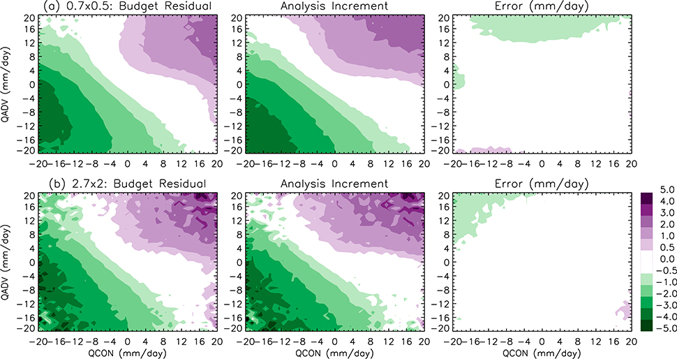
The errors from finite differencing and conversion of temporal and spatial resolutions can be estimated by the departures of the residuals of Eq. (1) (i.e., P − E + ∂Q/∂t − QCON − QADV) from the analysis increments. Figure 1 shows that such errors are in general less than 1 mm day⁻¹ for both the hourly dataset at native resolution (Fig. 1a) and the 3-hourly dataset at 2° × 2.7° resolution (Fig. 1b).

FIG. 1.

MERRA atmospheric-water-budget-related variables (mm day⁻¹) averaged on the phase space for (a) native resolution (⅔° × ½° × 1 hourly) and (b) resolution at 2.7° × 2° × 3 hourly (averaged 4 × 4 native grid cells). (left) The water budget residuals (P − E + ∂Q/∂t − QCON − QADV); (center) the MERRA analysis increments for Q; and (right) error estimates for finite differencing calculations [difference between (left) and (right)]. The phase space is spanned by QCON (abscissa) and QADV (ordinate).

We also calculate QCON and QADV using the European Centre for Medium-Range Weather Forecasts interim reanalysis (ERA-Interim, hereinafter ERAi; Dee et al. 2011) so that differences between reanalysis datasets can be assessed and used as uncertainty estimates of the references. ERAi 6-hourly data are averaged onto 2° latitude × 2° longitude grid boxes for comparison with the MERRA and GISS-E2 results. The difference in temporal resolution of ERAi from MERRA and GISS-E2 does not influence key results of this study.

b. Large-scale dynamical conditions in the water-budget-related phase space

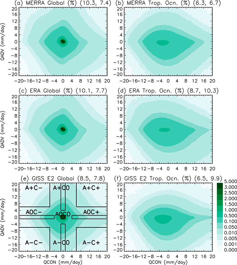
Joint histograms of three years’ (2007–09) QCON and QADV are plotted for MERRA, ERAi, and GISS-E2 in Figs. 2a,c,e for the whole globe and in Figs. 2b,d,f for the tropical oceans. All three models show the most frequent events at the center (hereafter referred to as the “quiet zone,” where QCON ≅ 0 and QADV ≅ 0) and along the pure convergence/divergence axis (QADV = 0) or the pure moist/dry advection axis (QCON = 0). Events of mixed combinations of large values of QCON and QADV are relatively rare. For the distribution over the tropical oceans, one sees higher skewness toward positive QCON because of the intertropical convergence zone (ITCZ), and toward negative QADV because of dry advection associated with the tropical trade winds.

FIG. 2.

Joint histograms of QCON (mm day⁻¹) and QADV (mm day⁻¹) for (a),(b) MERRA, (c),(d) ERAi, and (e),(f) GISS-E2 for 2007–09. Standard deviations of QCON and QADV are listed in the titles of each panel. The color shading indicates the probability (%) for (left) over the whole globe and (right) over the tropical oceans. Different dynamical regimes are defined by black boxes in (e) and labeled as A+C−, A+C0, A+C+, A0C−, A0C0 (the quiet zone), A0C+, A−C−, A−C0, and A−C+.

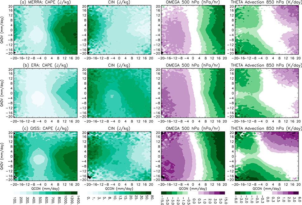
To demonstrate how tropical large-scale dynamical conditions vary in regimes in the phase space, averages of commonly used climate variables on the phase space are shown for MERRA (Fig. 3a), ERAi (Fig. 3b), and GISS-E2 (Fig. 3c) over the tropical oceans. These variables are convective available potential energy [CAPE (J kg⁻¹); Fig. 3, left], convective inhibition [CIN (J kg⁻¹); Fig. 3, center left], vertical velocity ω at 500 hPa [ω500 (hPa h⁻¹); Fig. 3, center right], and potential temperature advection at 850 hPa (−V · ∇θ, where θ is potential temperature; Fig. 3, right). CAPE measures the maximum kinetic energy an air parcel can gain through lifting by buoyancy in convection and, hence, how conditionally unstable the atmospheric column is. CIN measures the energy an air parcel needs to reach the free convection level in order to trigger deep convection and, hence, how stable the boundary layer is. The ω at 500 hPa is normally used to indicate if a large-scale grid cell in the tropics is strongly convective and is related to precipitation intensity and cloud properties in previous studies (e.g., Bony et al. 2013; Su et al. 2013). Low-level temperature advection can influence the development of convection in the tropics and is mainly contributed from regions poleward of 15° latitude in both hemispheres (because the temperature gradient is relatively small in the deep tropics).

FIG. 3.

Large-scale dynamical conditions over the tropical oceans averaged in the phase space for (a) MERRA, (b) ERAi, and (c) GISS-E2. (left) CAPE (J kg⁻¹), (center left) CIN (J kg⁻¹), (center right) vertical velocity at 500 hPa (hPa h⁻¹), and (right) horizontal advection of potential temperature at 850 hPa (K day⁻¹).

The three models have qualitatively similar distributions of these dynamical variables in the phase space. Variables commonly used to represent conditional stability (Bony and Dufresne 2005; Teixeira et al. 2011; Su et al. 2011, 2013), such as CAPE, CIN, and ω at 500 hPa, mainly vary in the direction of the QCON axis, with slight modulation by QADV. In the tropics, the sign of temperature advection is determined by the sign of QCON, with the absolute value of QADV modulating the magnitude. In the extratropics, regimes in the phase space with large moisture advection can be used to indicate baroclinic systems (see section 2c and Fig. 4).

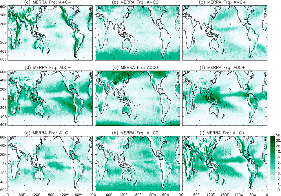
FIG. 4.

Geographical maps of occurrence frequencies (%) for the nine dynamical regimes defined in Fig. 2e using MERRA in 2007–09.

There are detailed quantitative differences among the three models for variables shown in Fig. 3. Differences in CAPE and CIN imply that temperature and/or specific humidity profiles are different among the models. Compared to the two reanalyses, GISS-E2 has stronger rising motion in conditionally unstable regimes and stronger sinking motion in regimes with boundary layers with strong inversions, implying a stronger Hadley (and/or Walker) circulation.

c. Dynamical regimes

Climate variables over the tropical oceans stratified as continuous functions of QCON and QADV can be directly associated with the large-scale dynamical conditions shown in Fig. 3. Given the patterns shown in Fig. 3, we examine in this study nine representative dynamical regimes with their boundaries shown in Fig. 2e to isolate various combinations of negative (−), near-zero (0), and positive (+) values of QADV (A) and QCON (C). The ranges of QCON and QADV for the nine regimes are listed in Table 1. Two regimes (A0C+ and A0C−) along the QCON axis have minimal effects from temperature and moisture advection but with strong conditional instability (A0C+) and low-level inversion (A0C−) associated with strong ascending and descending motion, respectively. Regimes A+C0 and A−C0 along the QADV axis have minimal effects of stability or vertical motion but with strong moist and dry advection, respectively. The regimes at the four corners (A+C+, A+C−, A−C−, and A−C+) have mixed effects of maximal moisture and temperature advections as well as dynamical convergence or divergence. The quiet zone (A0C0) has minimal effects from stability and moisture advection with near-zero vertical velocity at 500 hPa.

TABLE 1.

Acronyms of nine water-budget-related dynamical regimes and examples of dynamical systems they contain.

Regimes	Definitions (units in mm day−1)	Dynamical systems
A+C−	QADV > 6, QCON < −6	Mountainsides with uplifting motion.
A+C0	QADV > 6, −1 < QCON < 1	Extratropical eddies (poleward moist advection).
A+C+	QADV < 6, QCON < 6	Extratropical storm tracks and extreme precipitation.
A0C−	−1 < QADV < 1, QCON < −6	Subtropical stable boundary layer.
A0C0	−1 < QADV < 1, −1 < QCON < 1	Dry regions: deserts and polar air intrusion.
A0C+	−1 < QADV < 1, QCON > 6	ITCZ and SPCZ.
A−C−	QADV < −6, QCON < −6	Shallow convection.
A−C0	QADV < −6, −1 < QCON < 1	Shallow convection and extratropical eddies (equatorward dry advection).
A−C+	QADV < −6, QCON > 6	Mountain lee sides and dry air intrusion in ITCZ or SPCZ.

Geographical maps of occurrence frequencies for the nine dynamical regimes (Fig. 4) indicate that they are associated with familiar systems on the globe. ERAi and GISS-E2 have similar patterns in the geographical distributions, and we only show the MERRA distributions for purposes of illustration. The quiet zone (A0C0; Fig. 4e) has high occurrence frequencies in areas with weak moisture sources and sinks (e.g., deserts over land, the eastern parts of subtropical ocean basins, and polar regions). The regime A0C+ (strong convergence, weak advection; Fig. 4f) clearly identifies the ITCZ, where deep convective events frequently occur, while the regimes A−C− and A−C0 (strong dry advection with either strong or weak divergence; Figs. 4g and 4h, respectively) capture the subtropical subsidence regions on either side of the ITCZ influenced by the trade wind–induced dry air intrusion. Regimes A+C− (Fig. 4a) and A−C+ (Fig. 4i) are most common in coastal regions and especially in locations of orographic lifting and descent; the regime A+C− occurs infrequently over the tropical oceans, but the regime A−C+ is observed on occasion in the ITCZ and South Pacific convergence zone (SPCZ), perhaps in connection with subtropical dry air intrusions into convective regions (Lintner and Neelin 2008; Niznik and Lintner 2013). Regimes A+C+ and A+C0 (Figs. 4c,b) rarely occur in the tropics; in the extratropics, these regimes are common in the storm tracks associated with synoptic scale weather systems. The regime A0C− (strong divergence, weak advection; Fig. 4d) indicates regions of boundary layers with strong inversions in the eastern parts of subtropical oceans where stratus and stratocumulus are common. Meteorological or large-scale dynamical systems represented by the nine dynamical regimes are summarized in Table 1.

In the next section, we investigate how subgrid-scale cloud properties are modified by large-scale moisture tendencies by embedding these cloud properties in the phase space.

3. Clouds linked to large-scale dynamical conditions and atmospheric water budget

a. Representation of clouds

Following Rossow and Schiffer (1999), we represent clouds using retrievals of cloud-top pressure (CTP) and cloud optical depth (COD) from the Moderate Resolution Imaging Spectroradiometer (MODIS) collection 5.1 cloud products onboard the Aqua platform (MYD06c5.1; King et al. 2013; King et al. 2003; Platnick et al. 2003; Ackerman et al. 2008; Frey et al. 2008; Menzel et al. 2008). MODIS has a much smaller occurrence of middle clouds on a CTP–COD histogram than is seen by the ISCCP in cases when high-level clouds overlap low-level clouds (e.g., Chen and Del Genio 2009; Bodas-Salcedo et al. 2011). We average MODIS COD retrieved on 1-km pixels to 5-km resolution, on which the CTP is reported. The averaging is done by excluding pixels of zero COD, known as in-cloud averaging. Tests show that in-cloud averaging of COD preserves the patterns of CTP–COD histograms (Wong et al. 2015).

We define cloud state at each 5-km pixel by a pair of variables (CTP, COD). Each pair of MODIS CTP and COD is associated with a large-scale dynamical state by choosing the MERRA 2° × 2.7° grid cell that contains the MODIS 5-km pixel at the time closest to the MODIS overpass time. As a MERRA grid cell can include multiple MODIS 5-km pixels, one point in the phase space at a MERRA grid cell matched in time to MODIS is mapped to a histogram of MODIS cloud state distribution.

To represent cloud property statistics in GISS-E2 compatible to what the MODIS observes, the model clouds are processed by the Cloud Feedback Model Intercomparison Project (CFMIP) Observation Simulator Package (COSP) MODIS simulator (Bodas-Salcedo et al. 2011; Pincus et al. 2012). The simulator mimics instrument measurements at pixel scales by constructing subcolumns in each grid cell of the climate model and then samples subgrid-scale cloud properties from the subcolumns (Klein and Jakob 1999; Räisänen et al. 2004). A cloud in each subcolumn at each model level is treated as homogeneous, and the statistics of cloud properties (e.g., cloud fraction and cloud liquid and ice water contents) over all subcolumns at each model level are consistent with those of the grid-scale outputs. The cloud overlapping scheme used in the model is used to distribute the model clouds among the subcolumns.

COD in each subcolumn is the integrated liquid and ice water extinction from the surface to the top of atmosphere, and CTP in each subcolumn is determined by the mean extinction-weighted pressure of the first COD [see Eq. (2) in Pincus et al. (2012)]. Joint histograms of CTP and COD are aggregated for each model grid cell at each 3-hourly time step. For comparison with MODIS daytime observations, we analyze both dynamical and cloud-related data in each grid cell at the 3-hourly interval closest to 1330 local time. We have tested that daily averaged dynamical data yield results almost identical to what we will report in this study; however, we will present the results for the finer temporal resolution for increased robustness.

Occurrence frequencies of cloud state are calculated as fractions of each cloud state counts relative to the total counts in a histogram. Counts of clear sky in the MODIS observations are determined by the MODIS cloud mask (Ackerman et al. 1998; Frey et al. 2008). Counts of clear sky in one GISS-E2 model grid cell (at 2° × 2.5° resolution) are calculated as one minus the grid cloud fraction, and counts of a particular cloud state are the values given by the joint histogram from the MODIS simulator. All statistics of occurrence frequencies of cloud states are reported as joint histograms of CTP and COD (in percent), with the occurrence frequencies of clear sky specified.

b. Cloud responses to large-scale atmospheric water tendencies

Clouds created by a particular process in a climate model may have values of CTP and COD that are different from those in the real world. Thus, cloud type classification schemes designed for observational measurements (e.g., Rossow and Schiffer 1999) may not be directly applicable to climate model output. For comparison between observations and model results we avoid using fixed regions in the CTP–COD space to define cloud types, and instead we investigate the whole CTP–COD histograms and see how they change in different regimes of the phase space. The dynamical regimes defined in section 2c (or Fig. 2e) have geographical distributions (Fig. 4) of occurrence resembling certain cloud types. Therefore, as a first example, we investigate the CTP–COD histograms in the nine dynamical regimes.

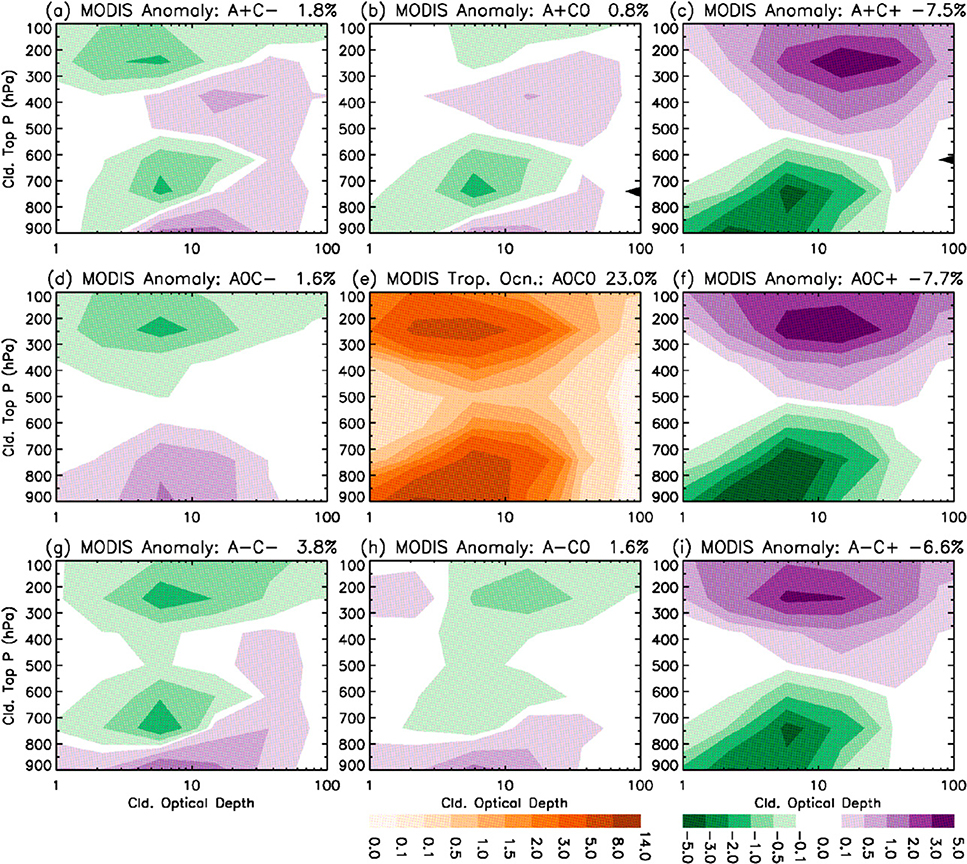
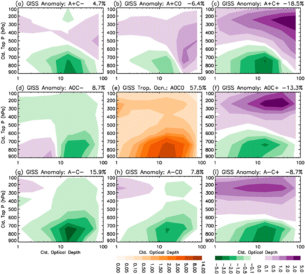
We quantify the changes of MODIS CTP–COD histograms when the large-scale dynamical conditions shift from the quiet zone (i.e., the center of the phase space). For this purpose, anomalies in CTP–COD histograms from those of the quiet zone are constructed for different dynamical regimes. These cloud histogram anomalies account for the formation or elimination of certain cloud states associated with changes in large-scale dynamical conditions. The same analysis is then applied to CTP–COD histograms from the COSP MODIS simulator implemented in GISS-E2. The phase space constructed from MERRA data is used to define the dynamical regimes for MODIS clouds, while GISS-E2 clouds are associated with its own model water budget tendencies. The results reported in this section are not sensitive to whether ERAi or MERRA water budget tendencies are used for the MODIS clouds. Figure 5 shows plots for the MODIS CTP and COD data, and Fig. 6 plots for data from the GISS-E2 COSP MODIS simulator.

FIG. 5.

Cloud state histograms (occurrence frequencies, %), spanned by MODIS CTP (ordinate) and COD (abscissa), sorted by the nine dynamical regimes over the tropical oceans. (e) The histogram for the quiet zone with the clear sky occurrence frequency shown in the panel title. Panels surrounding (e) are anomalous occurrence frequencies from those of the quiet zone for the other eight dynamical regimes, with the anomalous clear sky occurrence frequencies shown in the corresponding panel titles. The dynamical regimes are defined by the MERRA QCON and QADV. The labels of the nine dynamical regimes are in the panel titles, and the regimes defined in Fig. 2e.

FIG. 6.

As in Fig. 5, but for cloud state histograms calculated by the COSP MODIS simulator implemented in GISS-E2. The clear sky occurrence frequencies are calculated by the modeled total cloud fractions.

For the quiet zone (A0C0), the MODIS cloud CTP–COD histogram (Fig. 5e) shows a typical pattern with two maxima: one located at CTP around 200–300 hPa with COD around 2–10, the other located in the lower troposphere (CTP > 700 hPa) with COD in about the same range of the high-level maximum. The GISS-E2 simulated cloud occurrence frequencies for the quiet zone (Fig. 6e) qualitatively capture the pattern of the MODIS histogram, with the maxima located at thicker COD range (~10–24) for both high- and low-cloud regimes, and with fewer high clouds than MODIS. GISS-E2 has an additional maximum for high thin clouds (CTP in 200–400 hPa and COD ≤ 1) not observed by MODIS. While GISS-E2 contains thicker clouds, the clear sky occurrence frequency in the quiet zone (~58%) is more than twice the MODIS value (~23%).

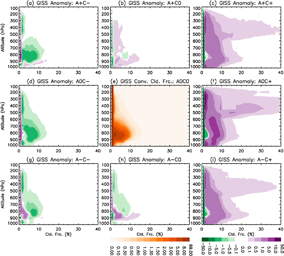
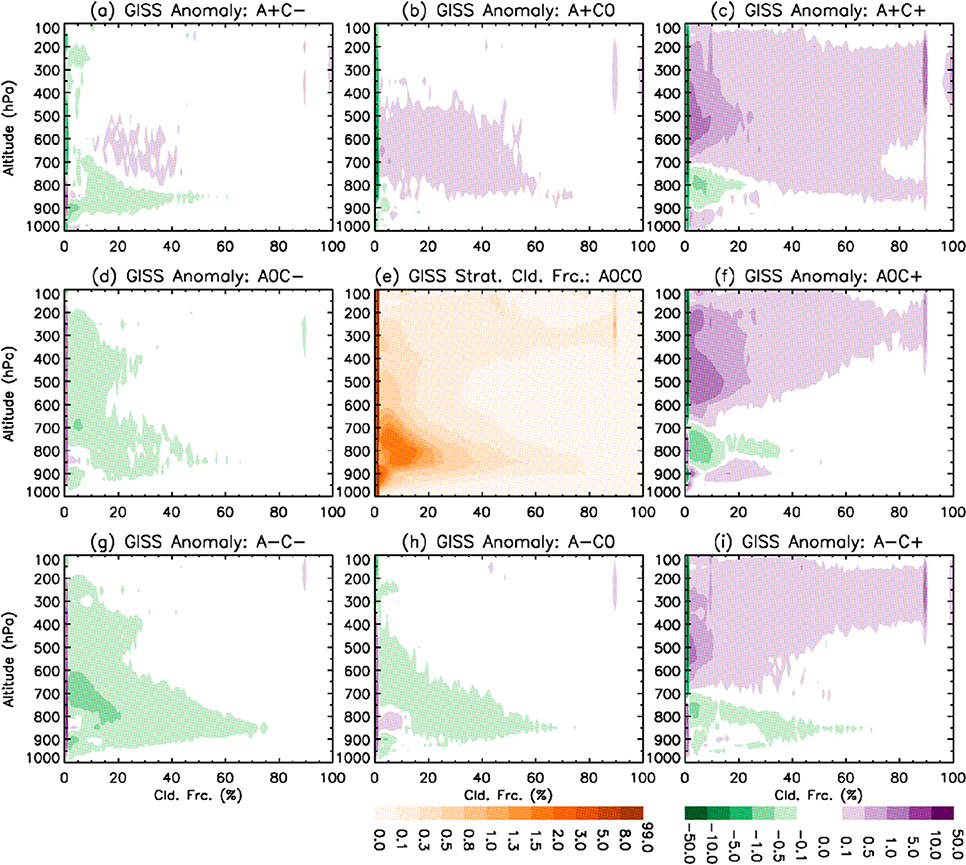
Further investigation of the diagnostics of convective (Fig. 7) versus stratiform (Fig. 8) cloud types in GISS-E2 helps understand the difference between the outputs of the simulator and the MODIS histograms. The low-level clouds in the GISS-E2 quiet zone are mainly shallow convective clouds with cloud fractions less than 10% (Fig. 7e) and stratiform clouds with cloud fractions occasionally reaching as high as 80% (Fig. 8e). The high-level clouds in the model quiet zone are mainly stratiform including cirrus. Because MODIS retrievals for COD < 1.3 have large discrepancies from those of ISCCP (Pincus et al. 2012) and MODIS COD limitation for cloud masks is COD < 0.4 (Ackerman et al. 2008), these thin clouds simulated in GISS-E2 may exist and are not detected by MODIS.

FIG. 7.

Histograms (occurrence frequencies, %) of GISS-E2 convective cloud fractions (%) as functions of altitudes sorted by the nine dynamical regimes. (e) The histogram for the quiet zone and normalized to 100% at each altitude level. Panels surrounding (e) are anomalous occurrence frequencies from those of the quiet zone (summed to zero at each altitude level) for the other eight dynamical regimes. The labels of the nine dynamical regimes are in the panel titles, and the regimes defined in Fig. 2e.

FIG. 8.

As in Fig. 7, but for histograms (occurrence frequencies, %) of GISS-E2 stratiform cloud fractions (%).

In the regimes of convergence (QCON > 0, regimes A+C+, A0C+, and A−C+; Figs. 5c,f,i), more high-level thick clouds (deep convective clouds) with histogram distributions skewing toward high-level intermediate to thin COD (Figs. 5c,f,i and 6c,f,i) are observed by MODIS. This reflects the fact that cirrus or cirrostratus clouds are associated with deep convective clouds by detrainment. GISS-E2 captures the feature of increasing COD with QADV (Figs. 6c,f,i), with thin to medium-thickness stratiform clouds (Figs. 8c,f,i) accompanying deep convective clouds (Figs. 7c,f,i). GISS-E2 has thicker COD and longer tails toward the thin ends of the high-cloud histograms when compared to MODIS.

Moist advection does modulate cloud properties in regimes of convergence (e.g., during intraseasonal oscillations) and divergence (transition from stratocumulus to cumulus clouds). To demonstrate the effects of moist and dry advection on cloud distributions, differences of cloud state histograms in Figs. 5 and 6 are calculated between the regimes of QADV > 0, QADV ≈ 0, and QADV < 0 for both regimes of convergence (QCON > 0) and divergence (QCON < 0).

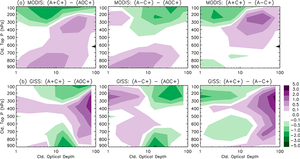
Moist advection in a regime of convergence is associated with more frequent low-level medium-thickness to thick clouds as well as thicker high clouds with lower cloud tops (Fig. 9a, left). Dry advection is associated with more low-level thin to medium-thickness clouds and high-level thin clouds (Fig. 9a, center). GISS-E2 qualitatively reproduces the modulation by moist advection (Fig. 9b), but with thicker high-level clouds that extend to lower altitudes and more high-level thin clouds. GISS-E2 also has less frequent low-level thin to medium-thickness clouds, probably related to its more high-level clouds that mask the low-level clouds in the COSP MODIS simulator.

FIG. 9.

Effects of moist advection on cloud state histograms in regimes of convergence (QCON > 0). (a) The MODIS cloud histograms (from Fig. 5) and (b) the cloud histograms from the COSP MODIS simulator in GISS-E2 (from Fig. 6). (left) The differences of the histograms between regimes A+C+ and A0C+, (center) the differences between regimes A−C+ and A0C+, and (right) the difference between (left) and (center).

In regimes of pure divergence (A0C−), the MODIS cloud occurrence frequency anomalies (Fig. 5d) show reasonable enhancement of low-level, medium-thickness to thick clouds (i.e., stratocumulus and stratus; COD > 3), marking the regions of boundary layer inversion over the eastern parts of subtropical ocean basins (Fig. 4d). GISS-E2 (Fig. 6d) also has more frequent low-level clouds in this dynamical regime but with much thinner COD than those shown in MODIS. There is less frequent occurrence of low-level thick clouds in GISS-E2 in contrast to what is observed by MODIS. In Figs. 7d and 8d we can see that both convective and stratiform clouds with large cloud fractions are much reduced, and the more frequent low-level, thin clouds seen in the MODIS simulator are mainly shallow convective clouds with cloud fractions less than 10%. This difficulty of simulating low-level medium to thick stratiform clouds in GISS-E2 exists in virtually all GCMs and is consistent with previous findings (e.g., Zhang et al. 2005; Nam et al. 2012; Su et al. 2013).

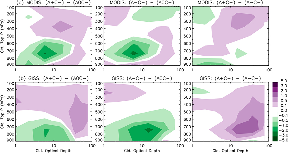
Moist advection in a divergent regime (QADV > 0; Fig. 10a, left, or cf. Figs. 5a and 5d) is associated with more medium-thickness clouds (10 < COD < 20) in the upper midtroposphere (300–500 hPa) and more medium-thickness low clouds, compared to the pure divergent regime (QADV ≈ 0). GISS-E2 captures the formation of midlevel stratiform clouds (Fig. 8a) in this regime as observed by MODIS but with thicker CODs (COD > 30; Fig. 6a or Fig. 10b, left) than those observed by MODIS (COD ≃ 10–40; Fig. 5a or Fig. 10a, left).

FIG. 10.

As in Fig. 9, but for the effects in regimes of divergence (QCON < 0). (left) The differences of the histograms between regimes A+C− and A0C−, (center) the differences between regimes A−C− and A0C−, and (right) the differences between (left) and (center).

Dry advection in the divergent regime (QADV < 0; Fig. 10a, center, or cf. Figs. 5g and 5d) is associated with more high-level thin clouds as well as low-level thin clouds with lower cloud tops. In fact the regime A−C− has the most frequent cumulus cloud and clear sky occurrence among the nine dynamical regimes. GISS-E2 qualitatively captures the most frequent occurrence of clear sky in the A−C− regime (Fig. 6g) but with much less frequent occurrence of low-level clouds and higher occurrence frequencies of high-level, thin clouds than MODIS (Fig. 10b, center, or cf. Figs. 6g and 5g). However, GISS-E2 model diagnostics for the regime A−C− (Fig. 7g) clearly indicate that there are more frequent convective low-level clouds in GISS-E2 with CTP > 800 hPa and cloud fractions less than 15%. This contrast between the model-diagnosed low-level convective clouds and the low-level cloud occurrence frequencies from the COSP MODIS simulator suggests that existence of high-level clouds can mask the detection of low-level clouds in the MODIS simulator. This is plausible in the cases of multilayer clouds when the CTPs are located at high altitudes by the MODIS simulator. Therefore, the elevated cloud tops of low-level thin clouds by moist advection as observed by MODIS (Fig. 10, right) are not present in the MODIS simulator.

In the regimes with QCON ≈ 0 (A0C0, A+C0, and A−C0; Fig. 5, center), occurrence of low-level thick clouds is less frequent as reported in many studies (e.g., Bony and Dufresne 2005; Teixeira et al. 2011; Su et al. 2011, 2013). Changes in cloud frequencies in these regimes are similar to those in the regimes of QCON < 0, with more frequent occurrence of low-level, thin clouds associated with shallow convection with dry advection (QADV < 0, A−C0; Fig. 5h) and more midlevel medium-thickness clouds with moist advection (QADV > 0, A+C0; Fig. 5b). The shallow convective clouds in GISS-E2 (Fig. 7h) are again masked by the more frequent high-level thin clouds in the MODIS simulator (Fig. 6h). GISS-E2 can also reproduce the more frequent midlevel to low-level stratiform clouds (Fig. 8b) but with COD thicker than those seen in MODIS (cf. Figs. 5b and 6b).

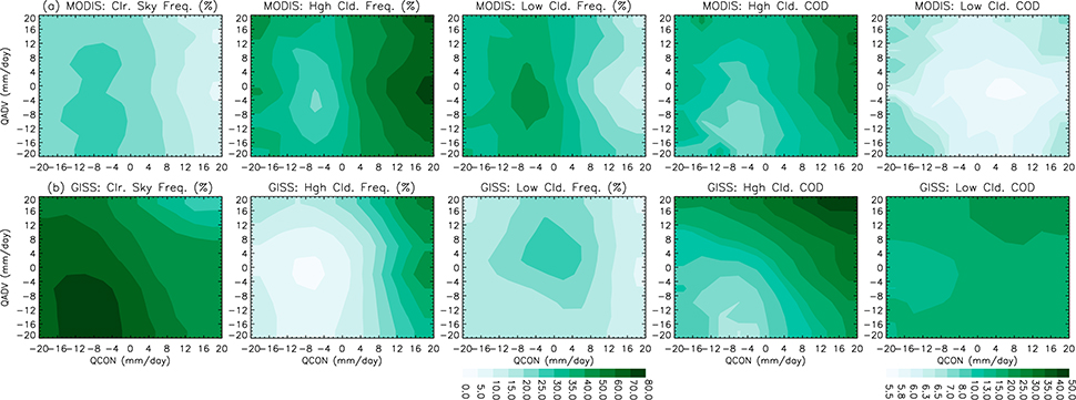
Figures 5 and 6 show cloud property histograms in nine distinct regimes in the phase space as examples of how moisture tendencies may modify the histograms. In fact, the cloud property histogram is a continuous function in the phase space. Therefore, we show in Fig. 11 comparisons between MODIS and GISS-E2 for clear sky, high- (CTP < 440 hPa) and low-level (CTP > 680 hPa) cloud occurrence frequencies together with their mean COD.

FIG. 11.

Cloud properties as functions of QCON and QADV for (a) MODIS and (b) GISS-E2. (left) Clear sky cloud frequencies, (left center) high cloud frequencies, (center) low cloud frequencies, (right center) mean high cloud COD, and (right) mean low cloud COD. The color bar at bottom center is for cloud frequencies (first three panels from left to right) and at bottom right is for mean COD (last two panels).

MODIS cloud masks indicate that clear sky (Fig. 11a, left) is more frequent as divergence increases with slight modulation by moist advection. In GISS-E2 (Fig. 11b, left), clear sky has higher occurrence frequencies and increases by both divergence and dry advection. High-level cloud occurrence frequencies (Fig. 11a, left center) increase with convergence, with modulation by moist advection. GISS-E2 reproduces qualitative features of the MODIS distributions of high-level cloud occurrence frequencies (Fig. 11b, left center), although the overall frequencies are smaller than MODIS. Low-level clouds occur more frequently in GISS-E2 over regimes of small convergence or divergence with moist advection (Fig. 11b, center), in contrast to regimes of divergence in MODIS (Fig. 11a, center).

The high-level mean COD (Fig. 11a, right center) has distributions in the phase space similar to cloud frequencies (Fig. 11a, left center), with the thinnest clouds occurring in regimes with dry advection and moderate divergence and the thickest clouds occurring in regimes when both convergence and moist advection are large. GISS-E2 reproduces qualitative features of the MODIS distributions of high-level mean COD but with overall thicker clouds than MODIS. The model dependence of low-level mean COD on QCON and QADV is different from those of MODIS (Fig. 11, right), as is the model low-level cloud frequencies (Fig. 11, center). Reasons behind these model discrepancies are still unclear, as described in many previous studies (e.g., Zhang et al. 2005; Nam et al. 2012; Su et al. 2013).

c. Precipitation linked to clouds and large-scale dynamical conditions

Precipitation [P in Eq. (1)] is tightly linked to clouds and large-scale dynamical conditions. We investigate in this section how P over the tropical oceans is distributed in the phase space. The Global Precipitation Climatology Project (GPCP)1° daily (1DD, version 1.2; data can be downloaded from http://precip.gsfc.nasa.gov) precipitation product (Huffman et al. 2001) is used to evaluate the precipitation of MERRA, ERAi, and GISS-E2. The GPCP 1DD precipitation is based on the GPCP version 2.2 satellite–gauge product, which merges global precipitation gauge analyses with precipitation retrievals from satellites, including Special Sensor Microwave Imager and Imager/Sounder (SSM/I and SSMIS), Television Infrared Observation Satellite (TIROS) Operational Vertical Sounder (TOVS), AIRS, and others (Adler et al. 2012; Huffman et al. 2001, 2009). To facilitate the comparison to GPCP precipitation, the model precipitation and water budget tendencies are averaged daily.

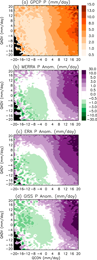
Compared to the GPCP 1DD precipitation data (Fig. 12), MERRA, ERAi, and GISS-E2 all have higher precipitation in dynamical conditions favoring strong precipitation and lower precipitation in conditions favoring weak precipitation. While there are discrepancies in global precipitation estimates (Behrangi et al. 2014), the tropical mean precipitation discrepancies (20%–43%) are beyond the most updated bias estimates for GPCP (4%–6%; A. Behrangi 2016, personal communication) and also larger than the highest value of missed precipitation (10%–20%) estimated from the global energy balance (Stephens et al. 2012).

FIG. 12.

Comparisons of daily precipitation (mm day⁻¹) over the tropical ocean from the models to the observations on the phase space. The observation is (a) the GPCP 1DD precipitation averaged on the phase space. The corresponding anomalies of the modeled precipitation relative to the GPCP are (b) for MERRA, (c) for ERAi, and (d) for GISS-E2.

4. Conclusions and discussion

The two tendency terms related to dynamical convergence (QCON ≡ −Q∇ · V) and moist advection (QADV ≡ −V · ∇Q) in the atmospheric water budget equation [see Eq. (1)] are used to define the water-budget-related phase space. With QADV as an additional degree of freedom, the phase space represents not only those commonly used parameters sensitive to largescale convergence but also those associated with the changes of low-level moist advection. Climate variables compared among different models or against observations in the phase space share the same reference of the atmospheric water budget that is linked to large-scale dynamical conditions.

Along the dimension of QCON, large-scale conditions change from regimes with strong boundary layer inversion and descending motion to regimes of high conditional instability and ascending motion. Fluctuations in moisture advection not only generate fluctuations in precipitation (e.g., Wong et al. 2011) but also modulate cloud type distributions (e.g., Del Genio et al. 2012, 2015; Wang et al. 2015). The effects of QCON and QADV on cloud type distributions and precipitation over the tropical oceans can be described in the phase space and be used to evaluate those simulated in the climate model.

GISS-E2 clear sky and high-level cloud frequencies as well as the high-level COD means have distributions in the phase space qualitatively similar to those of MODIS, although GISS-E2 has more frequent clear sky with thicker clouds. GISS-E2 has less frequent occurrence of low-level clouds of thicker COD, consistent with the “too few, too bright problem” shared with almost all climate models (Nam et al. 2012). Low-level clouds in GISS-E2 are most abundant in regimes of near-zero convergence and moist advection (QADV > 0), in contrast to the regimes of divergence (QCON < 0) as observed in MODIS. Although GISS-E2 properly generates shallow convection in regimes of divergence and dry advection, the more abundant high clouds in GISS-E2 mask the existence of low-level, thin clouds in the COSP MODIS simulator. It is not known yet if the more frequent high-level, thin clouds in GISS-E2 are realistic because MODIS has limitations in detecting thin clouds (Ackerman et al. 2008; Pincus et al. 2012). These limitations hinder the evaluation of frequencies of both high- and low-level thin clouds in GISS-E2 against retrievals from passive imagers (either MODIS or ISCCP). Future investigation using CloudSat/CALIPSO is necessary.

In regimes of convergence, moist and dry advection modulate the anomalies in abundance of high-level thick and low-level thin to medium-thickness clouds (Fig. 9a). GISS-E2 can capture such modulation with thicker high-level clouds that extend to lower altitudes and with smaller anomalies in low-level cloud frequencies, probably related to its larger anomalies in high-level thin cloud frequencies.

In regimes of divergence, moist and dry advection modulate the cloud tops of low-level thin to medium-thickness clouds and the abundance of high- to midlevel medium-thickness to thick clouds. GISS-E2 captures similar modulation for high- to midlevel clouds but with thicker optical depth. The effects of moist advection on low-level clouds are not seen in the COSP MODIS simulator, probably related to the more abundant high-level thin clouds in GISS-E2 that mask the existence of low-level thin clouds.

Precipitation strongly increases with convergence, with slight modulation by moist advection. MERRA, ERAi, and GISS-E2 have more precipitation compared to GPCP 1DD product in regimes of heavy rain but less precipitation in regimes of light rain.

Although our study is focused on general climatologies over the tropical oceans, the water-budget-related phase space is applicable to specific phenomena. For example, over the Indian subcontinent, evolution of cloud state distributions at the intraseasonal time scale is linked to anomalies in atmospheric water budget in the phase space. Positive moisture advection anomalies define the preconditioning phase for transition of shallow to deep convection (Wang et al. 2015). In the extratropics, the regime of large convergence and moist advection (A+C+) identifies midlatitude storm tracks (Fig. 4c). How the phase space can be used to describe clouds and precipitation related to extratropical cyclones needs further study.

REFERENCES

- Ackerman SA, Strabala KI, Menzel WP, Frey RA, Moeller CC, and Gumley LE, 1998: Discriminating clear sky from clouds with MODIS. J. Geophys. Res, 103, 32 141–32 157, doi: 10.1029/1998JD200032. [DOI] [Google Scholar]
- Ackerman SA, Holz RE, Frey R, Eloranta EW, Maddux B, and McGill M, 2008: Cloud detection with MODIS. Part II: Validation. J. Atmos. Oceanic Technol, 25, 1073–1086, doi: 10.1175/2007JTECHA1053.1. [DOI] [Google Scholar]
- Adler RF, Gu G, and Huffman GJ, 2012: Estimating climatological bias errors for the Global Precipitation Climatology Project (GPCP). J. Appl. Meteor. Climatol, 51, 84–99, doi: 10.1175/JAMC-D-11-052.1. [DOI] [Google Scholar]
- Behrangi A, Stephens G, Adler RF, and Huffman GJ, 2014: An update on the oceanic precipitation rate and its zonal distribution in light of advanced observations from space. J. Climate, 27, 3957–3965, doi: 10.1175/JCLI-D-13-00679.1. [DOI] [Google Scholar]
- Bodas-Salcedo A, and Coauthors, 2011: COSP: Satellite simulation software for model assessment. Bull. Amer. Meteor. Soc, 92, 1023–1043, doi: 10.1175/2011BAMS2856.1. [DOI] [Google Scholar]
- Bony S, and Dufresne J-L, 2005: Marine boundary layer clouds at the heart of tropical cloud feedback uncertainties in climate models. Geophys. Res. Lett, 32, L20806, doi: 10.1029/2005GL023851. [DOI] [Google Scholar]
- Bony S, Bellon G, Klocke D, Sherwood S, Fermepin S, and Denvil S, 2013: Robust direct effect of carbon dioxide on tropical circulation and regional precipitation. Nat. Geosci, 6, 447–451, doi: 10.1038/ngeo1799. [DOI] [Google Scholar]
- Bony S, and Coauthors, 2015: Clouds, circulation, and climate sensitivity. Nat. Geosci, 8, 261–268, doi: 10.1038/ngeo2398. [DOI] [Google Scholar]
- Bosilovich MG, Robertson FR, and Chen J, 2011: Global energy and water budgets in MERRA. J. Climate, 24, 5721–5739, doi: 10.1175/2011JCLI4175.1. [DOI] [Google Scholar]
- Chen Y, and Del Genio AD, 2009: Evaluation of tropical cloud regimes in observations and a general circulation model. Climate Dyn, 32, 355–369, doi: 10.1007/s00382-008-0386-6. [DOI] [Google Scholar]
- Colman R, 2003: A comparison of climate feedbacks in general circulation models. Climate Dyn, 20, 865–873, doi: 10.1007/s00382-003-0310-z. [DOI] [Google Scholar]
- Dee DP, and Coauthors, 2011: The ERA-Interim reanalysis: Configuration and performance of the data assimilation system. Quart. J. Roy. Meteor. Soc, 137, 553–597, doi: 10.1002/qj.828. [DOI] [Google Scholar]
- Del Genio AD, Chen Y, Kim D, and Yao M-S, 2012: The MJO transition from shallow to deep convection in CloudSat/CALIPSO data and GISS GCM simulations. J. Climate, 25, 3755–3770, doi: 10.1175/JCLI-D-11-00384.1. [DOI] [Google Scholar]
- Del Genio AD, Wu J, Wolf AB, Chen Y, Yao M-S, and Kim D, 2015: Constraints on cumulus parameterization from simulations of observed MJO events. J. Climate, 28, 6419–6441, doi: 10.1175/JCLI-D-14-00832.1. [DOI] [Google Scholar]
- Dessler AE, 2010: A determination of the cloud feedback from climate variations over the past decade. Science, 330, 1523–1527, doi: 10.1126/science.1192546. [DOI] [PubMed] [Google Scholar]
- Frey RA, Ackerman SA, Liu Y, Strabala KI, Zhang H, Key J, and Wang X, 2008: Cloud detection with MODIS. Part I: Recent improvements in the MODIS cloud mask. J. Atmos. Oceanic Technol, 25, 1057–1072, doi: 10.1175/2008JTECHA1052.1. [DOI] [Google Scholar]
- Huffman GJ, Adler RF, Morrissey M, Bolvin DT, Curtis S, Joyce R, McGavock B, and Susskind J, 2001: Global precipitation at one-degree daily resolution from multi-satellite observations. J. Hydrometeor, 2, 36–50, doi:. [DOI] [Google Scholar]
- Huffman GJ, Adler RF, Bolvin DT, and Gu G, 2009: Improving the global precipitation record: GPCP version 2.1. Geophys. Res. Lett, 36, L17808, doi: 10.1029/2009GL040000. [DOI] [Google Scholar]
- Kim D, Sobel AH, Del Genio A, Chen Y, Camargo SJ, Yao M-S, Kelly M, and Nazarenko L, 2012: The Madden–Julian oscillation and tropical cyclones simulated in the NASA GISS general circulation model. J. Climate, 25, 4641–4659, doi: 10.1175/JCLI-D-11-00447.1. [DOI] [Google Scholar]
- King MD, and Coauthors, 2003: Cloud and aerosol properties, precipitable water, and profiles of temperature and water vapor from MODIS. IEEE Trans. Geosci. Remote Sens, 41, 442–458, doi: 10.1109/TGRS.2002.808226. [DOI] [Google Scholar]
- King MD, Platnick S, Menzel WP, Ackerman SA, and Hubanks PA, 2013: Spatial and temporal distribution of clouds observed by MODIS onboard the Terra and Aqua satellites. IEEE Trans. Geosci. Remote Sens, 51, 3826–3852, doi: 10.1109/TGRS.2012.2227333. [DOI] [Google Scholar]
- Klein SA, and Jakob C, 1999: Validation and sensitivities of frontal clouds simulated by the ECMWF model. Mon. Wea. Rev, 127, 2514–2531, doi:. [DOI] [Google Scholar]
- Lintner BR, and Neelin JD, 2008: Eastern margin variability of the South Pacific convergence zone. Geophys. Res. Lett, 35, L16701, doi: 10.1029/2008GL034298. [DOI] [Google Scholar]
- Menzel WP, Frey RA, Zhang H, Wylie DP, Moeller CC, Holz RE, Maddux B, Baum BA, Strabala KI, and Gumley LE, 2008: MODIS global cloud-top pressure and amount estimation: Algorithm description and results. J. Appl. Meteor. Climatol, 47, 1175–1198, doi: 10.1175/2007JAMC1705.1. [DOI] [Google Scholar]
- Nam C, Bony S, Dufresne J-L, and Chepfer H, 2012: The ‘too few, too bright’ tropical low-cloud problem in CMIP5 models. Geophys. Res. Lett, 39, L21801, doi: 10.1029/2012GL053421. [DOI] [Google Scholar]
- Niznik MJ, and Lintner BR, 2013: Circulation, moisture, and precipitation relationships along the South Pacific convergence zone in reanalyses and CMIP5 models. J. Climate, 26, 10 174–10 192, doi: 10.1175/JCLI-D-13-00263.1. [DOI] [Google Scholar]
- Peixoto JP, and Oort AH, 1992: Physics of Climate. American Institute of Physics, 520 pp. [Google Scholar]
- Pincus R, Platnick S, Ackerman SA, Hemler RS, and Hofmann RJP, 2012: Reconciling simulated and observed views of clouds: MODIS, ISCCP, and the limits of instrument simulators. J. Climate, 25, 4699–4720, doi: 10.1175/JCLI-D-11-00267.1. [DOI] [Google Scholar]
- Platnick S, King MD, Ackerman SA, Menzel WP, Baum BA, Riedl JC, and Frey RA, 2003: The MODIS cloud products. Algorithm and examples from Terra. IEEE Trans. Geosci. Remote Sens, 41, 459–473, doi: 10.1109/TGRS.2002.808301. [DOI] [Google Scholar]
- Räisänen P, Barker HW, Khairoutdinov MF, Li J, and Randall DA, 2004: Stochastic generation of subgrid-scale cloudy columns for large-scale models. Quart. J. Roy. Meteor. Soc, 130, 2047–2067, doi: 10.1256/qj.03.99. [DOI] [Google Scholar]
- Randall DA, and Coauthors, 2007: Climate models and their evaluation Climate Change 2007: The Physical Science Basis, Solomon S et al. , Eds., Cambridge University Press, 589–662. [Google Scholar]
- Rienecker MM, and Coauthors, 2008: The GEOS-5 data assimilation system—Document of versions 5.0.1, 5.1.0, and 5.2.0. NASA Tech. Rep. NASA/TM-2008–104606, 116 pp. [Google Scholar]
- Rienecker MM, and Coauthors, 2011: MERRA: NASA’s Modern-Era Retrospective Analysis for Research and Applications. J. Climate, 24, 3624–3648, doi: 10.1175/JCLI-D-11-00015.1. [DOI] [PMC free article] [PubMed] [Google Scholar]
- Ringer MA, and Coauthors, 2006: Global mean cloud feedbacks in idealized climate change experiments. Geophys. Res. Lett, 33, L07718, doi: 10.1029/2005GL025370. [DOI] [Google Scholar]
- Rossow WB, and Schiffer RA, 1999: Advances in understanding clouds from ISCCP. Bull. Amer. Meteor. Soc, 80, 2261–2288, doi:. [DOI] [Google Scholar]
- Schmidt GA, and Coauthors, 2014: Configuration and assessment of the GISS ModelE2 contributions to the CMIP5 archive. J. Adv. Model. Earth Syst, 6, 141–184, doi: 10.1002/2013MS000265. [DOI] [Google Scholar]
- Soden BJ, and Held IM, 2006: An assessment of climate feedbacks in coupled ocean–atmosphere models. J. Climate, 19, 3354–3360, doi: 10.1175/JCLI3799.1. [DOI] [Google Scholar]
- Stephens, and Coauthors, 2012: An update on Earth’s energy balance in light of the latest global observations. Nat. Geosci, 5, 691–696, doi: 10.1038/ngeo1580. [DOI] [Google Scholar]
- Su H, Jiang JH, Teixeira J, Gettelman A, Huang X, Stephens G, Vane D, and Perun VS, 2011: Comparison of regime-sorted tropical cloud profiles observed by CloudSat with GEOS5 analyses and two general circulation model simulations. J. Geophys. Res, 116, D09104, doi: 10.1029/2010JD014971. [DOI] [Google Scholar]
- Su H, and Coauthors, 2013: Diagnosis of regime-dependent cloud simulation errors in CMIP5 models using “A-Train” satellite observations and reanalysis data. J. Geophys. Res. Atmos, 118, 2762–2780, doi: 10.1029/2012JD018575. [DOI] [Google Scholar]
- Teixeira J, and Coauthors, 2011: Tropical and subtropical cloud transitions in weather and climate prediction models: The GCSS/WGNE Pacific cross-section intercomparison (GPCI). J. Climate, 24, 5223–5256, doi: 10.1175/2011JCLI3672.1. [DOI] [Google Scholar]
- Trenberth KE, and Guillemot CJ, 1998: Evaluation of the atmospheric moisture and hydrological cycle in the NCEP/NCAR reanalysis. Climate Dyn, 14, 213–231, doi: 10.1007/s003820050219. [DOI] [Google Scholar]
- Wang T, Wong S, and Fetzer EJ, 2015: Cloud regime evolution in the Indian monsoon intraseasonal oscillation: Connection to large-scale dynamical conditions and the atmospheric water budget. Geophys. Res. Lett, 42, 9465–9472, doi: 10.1002/2015GL066353. [DOI] [Google Scholar]
- Webb MJ, and Coauthors, 2006: On the contribution of local feedback mechanisms to the range of climate sensitivity in two GCM ensembles. Climate Dyn, 27, 17–38, doi: 10.1007/s00382-006-0111-2. [DOI] [Google Scholar]
- Wong S, Fetzer EJ, Kahn BH, Tian B, Lambrigtsen BH, and Ye H, 2011: Closing the global water vapor budget with AIRS water vapor, MERRA reanalysis, TRMM and GPCP precipitation, and GSSTF surface evaporation. J. Climate, 24, 6307–6321, doi: 10.1175/2011JCLI4154.1. [DOI] [Google Scholar]
- Wong S, Fetzer EJ, Schreier M, Manipon G, Fishbein EF, Kahn BH, Yue Q, and Irion FW, 2015: Cloud-induced uncertainties in AIRS and ECMWF temperature and specific humidity. J. Geophys. Res. Atmos, 120, 1880–1901, doi: 10.1002/2014JD022440. [DOI] [Google Scholar]
- Zelinka MD, Klein SA, and Hartmann DL, 2012: Computing and partitioning cloud feedbacks using cloud property histograms. Part II: Attribution to changes in cloud amount, altitude, and optical depth. J. Climate, 25, 3736–3754, doi: 10.1175/JCLI-D-11-00249.1. [DOI] [Google Scholar]
- Zhang MH, and Coauthors, 2005: Comparing clouds and their seasonal variations in 10 atmospheric general circulation models with satellite measurements. J. Geophys. Res, 110, D15S02, doi: 10.1029/2004JD005021. [DOI] [Google Scholar]